Unterschrift des Betreuers
DIPLOMARBEIT
From Random Graphs to
Complex Networks:
A Modelling Approach
Ausgef¨uhrt am Institut f¨ur Diskrete Mathematik und Geometrie
der Technischen Universit¨at Wien
unter der Anleitung von Ao.Univ.Prof. Bernhard Gittenberger
durch
Christina Kn¨
obel
Herbeckstr. 46/6 1180 Wien
Acknowledgments
First and foremost, I would like to thank Professor Dr. Bernhard Gittenberger for being the adviser any student could hope for: He was patient, reliable, and encouraging and always took the time to answer all my questions. I also appreciated the chance to obtain invaluable teaching experience, as well as the vast number of letters of recommendation he wrote for me.
In addition, I would like to thank Dr. Matthias Dehmer for pointing me towards some papers on complex networks I might have missed, as well as Dipl.-Ing. Martins Bruveris, Dipl.-Ing. Johannes Morgenbesser and Dipl.-Ing. Andrea Trautsamwieser for their helpful and motivating comments.
Special thanks goes to Wolfgang M¨uller for meticulously proof-reading my diploma thesis, fine-tuning my computer, and being a friend.
Contents
1 Introduction 7
1.1 Some Notes on the Models . . . 7
1.1.1 State of the Art . . . 8
1.2 Graph Theoretical Preliminaries . . . 8
1.3 Properties of Complex Networks . . . 9
1.3.1 Big and Sparse . . . 10
1.3.2 The Small-World Effect . . . 10
1.3.3 The Clustering Coefficient . . . 10
1.3.4 Scale-free Networks . . . 11
2 Touching upon Real Networks 13 2.1 Social Networks . . . 13
2.2 Scientific Collaboration Networks . . . 14
2.3 The Internet and www . . . 16
2.3.1 The Internet . . . 16
2.3.2 The World Wide Web . . . 17
2.4 Brief Outlook . . . 18
3 Methods 21 3.1 Methods from Statistical Physics . . . 21
3.1.1 The Mean Field Method and other Continuum Approaches . . . 21
3.1.2 The Master Equation . . . 21
3.2 Methods from Probability Theory . . . 22
3.2.1 Some Distributions . . . 22
3.2.2 Two familiar Inequalities . . . 22
3.2.3 Markov Chains . . . 23
3.2.4 Martingales . . . 24
3.3 Notations and Abbreviations . . . 24
4 The “classical” Random Graph Model by Erd˝os and R´enyi 27 4.1 The Model . . . 27
4.2 Threshold Functions . . . 29
4.3 The Giant Component . . . 32
4.4 The Clustering Coefficient of Classical Random Graphs . . . 38
4.5 The Degree Sequence of Random Graphs . . . 41
4.6 The Diameter . . . 44
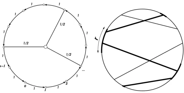
5 Small-World Networks 53 5.1 The Basic Idea . . . 53
5.2.1 A Toy Small-World Network . . . 54
5.2.2 The Mean-Field Solution . . . 56
5.3 Some Rigorous Approaches . . . 58
5.3.1 A Markov Chain Small-World Model . . . 58
5.3.2 Spatial Random Graphs . . . 61
6 Models with Preferential Attachment 65 6.1 The Preferential Attachment Model of Barab´asi and Albert . . . 65
6.2 First Calculations, Explanations, and Criticism . . . 66
6.2.1 A Mean-Field Approach . . . 66
6.2.2 Linear and Non-linear Preferential Attachment . . . 66
6.2.3 Some Problems with the Barab´asi-Albert Model . . . 67
6.3 An Extension of the Barab´asi-Albert Model . . . 68
6.4 Some Rigorous Results on Exact Models . . . 69
6.4.1 The Diameter and Clustering Coefficient of the LCD Model . . . 69
6.4.2 The Buckley-Osthus Model and the Degree Distribution . . . 73
7 More Models 77 7.1 The Copying Model . . . 77
7.2 The Cooper-Frieze Model . . . 78
7.3 Thickened Trees . . . 80
7.4 Protean Graphs . . . 83
1 Introduction
Recent years have seen an upsurge in the study of so-called “complex networks.” Various vast data bases are now available for investigation that were not given only a few years ago; they are mostly so large that research would not be possible without the help of very powerful, modern computers. Some examples are e-mail records, GPS navigation systems that capture travel patterns and the World Wide Web (www). Social Networks, which have been studied for a very long time already [23, 34], are now being looked into in a different way, i.e. through citation networks [2, 4, 17, 38]. All these examples would be called complex networks, and have influenced a major part of the work presented in this diploma thesis greatly.
To generalize from these examples, each consists of a very large set of objects that have some kind of relation to each other — that is, where the relation exists, it is the same type of relation between any pair of objects. (Compare for example with definition 2.1.) Mathematically, a network is nothing else than a graph [17].
The subject of this diploma thesis is the modelling of complex networks. The road map is as follows:
In this chapter, I will first state some basic graph theoretical preliminaries, and then go on to describe what typical properties of complex networks are, i.e. what we will be looking for in the models. This will be illustrated by motivating examples in chapter 2. Then, in chapter 3, I will briefly refresh some mathematical areas and state a few theorems used, and give explanations to some methods used by physicists. Chapter 4 will deal with the first model of random graphs, the Erd˝os-R´eyni model. It is fairly long, and is the chapter where theorems are given with rigorous proofs. Chapters 5 and 6 are more modern, dealing with models that try to put the complex networks as we understand them at the time into models. If available, an outline of the proofs will be given. Finally, chapter 7 mentions some other models that were very important in the forming of the theory of complex networks, as well as some newer models.
1.1 Some Notes on the Models
There are several reasons to model these huge networks, and it is not only out of theoretical curiosity (Are they really random? Do they form according to a system?) that researchers have been striving to understand these interwoven systems [2].
Be it a model that could predict when a small power failure could lead to a major electricity shortage — see [46] — or an accurate model of the World Wide Web, the web graph, helping to solve problems that are computationally difficult directly on the web (for example, testing new algorithms [32]), the applications are manifold.
1.1.1 State of the Art
Bollob´as nicely summarized what type of investigations of complex networks exist in [10]. Briefly, there are
• direct investigations of real networks, where nodes, degrees and so forth are counted and various properties are examined.
• These studies are followed by new models that try to explain why the properties measured are what they are.
• Often these models are examined via computer simulations, • and/or a heuristic analysis of their properties.
• Very rarely in comparison, a mathematically rigorous study is successfully under-taken.
1.2 Graph Theoretical Preliminaries
Following definitions are necessary for the most basic understanding of this diploma thesis, and may be skipped if the basic concepts of graph theory are known to the reader. All definitions in this section are made with help of [8].
As stated above, a network is actually a graph:
Definition 1.1 (Graph). An undirected graph G(V, E) consists of an ordered pair of sets, the vertices (or nodes) V of a graph and the edges E of a graph, where E ⊂V(2), the set of unordered pairs of V.
Definition 1.2. A directed graphG(V, E) (also called digraph) also consists of an ordered pair of sets; the difference is that here E ⊂ V ×V, the set of ordered pairs of V. These elements of E are called arcs.
Most results will be brought for undirected graphs, thus when we write graph we mean an undirected graph. It will only be emphasized when a graph is directed.
When referring to the vertice or edge set of a certain graph G(V, E), we will speak of
V(G) orE(G), respectively. |G|is defined as |V(G)|.
Definition 1.3. An edge {u, v} joins (or connects, or links) the vertices u and v. It will also be denoted by uv. u is said to be a neighbor of v. These vertices are also called adjacent. u and vare both incidentwith the edgeuv. For an arc (u, v) in a directed graph, we say that the arc begins inu and ends at v.
Definition 1.4 (Multigraph). A graph that contains multiple edges and edges of the form {v, v}(so-called loops) is called a multigraph. A graph without loops containing no multiple edges is called simple.
Note that there are n2
possible edges in a simple, undirected graph. A graph where all possible edges are present is called acomplete graph; for |V(G)|=n, it is denoted byKn.
˜
G is said to be a subgraph of G if V( ˜G) ⊆ V(G) and E( ˜G ⊆ G). This is written as ˜
G⊆G. ForW ⊆V(G),G−W means deleting all vertices inW and all the edges adjacent to them. We will denote this by [G/W].
1.3 Properties of Complex Networks
Two graphsGandG′are calledisomorphicif there exists a bijective function Φ :V(G)→
V(G′) such that for every uv∈E(G), Φ(u)Φ(v)∈E(G′), we write this asG∼= ˜G
For a vertex v ∈V(G) we denote by d(v) the degree of this vertex: It is defined as the number of edges adjacent tov. Similarly, theout-degree dout(v) in a directed graph is the number of arcs that begin inv and thein-degree din(v) of a vertex vis the number of arcs that end inv.
A graphP of the formE ={v0v1, v1v2, . . . vn−1vn}is called apath. v0 is called the initial vertex ofP and vnthe end vertex. The number of edges in a path is called thepath length.
Ifv0 =vn thenP is called a circuit. If a circuit C does not have a vertex usuch that u is
used twice (i.e. viu∈E(C) and vju∈E(C),i6=j) C is called a cycle. A graph without a
cycle is called aforest.
The vertices of a graph that are reachable from each other via paths are said to be part of the sameconnected component. A graph where the largest connected component is the graph itself is said to be connected. A graph Gon nvertices, n large, whose greatest con-nected component consists oflvertices so that l=O(n) is said to have agiant component. A connected forest is called a tree. A recursive tree is defined to be a labelled tree that is formed via a graph process. Starting with node 1, theroot, each new vertex j connects to an older vertex of the system at timej so that the path from any vertex to the root is always ascending.
For Digraphs, we distinguish the strongly connected and weakly connected. The latter is the case when the digraph, seen as an undirected graph, is connected, for the former there must be directed paths from any vertex to any other vertex.
The diameter of a graph is defined as diamG= max {vi,vj}∈V×V min P⊂G P is a path fromvitovj |E(P)|.
Note that the diameter of an unconnected graph is usually said to equal infinity.
A graph is said to be bipartite if V can be partitioned into two disjoint sets V1 and V2 such that there exists no edge inE(G) that connects two vertices in the same set.
1.3 Properties of Complex Networks
There does not seem to exist an exact definition of what makes a network complex. Vaguely speaking, a network is called complex when it has, in some sense, generated itself (see chapter 2 for examples) without a “construction plan” to guide the evolution. In most complex networks, there is still a certain dynamic in the network itself — it is still growing (or perhaps shrinking) over time, it is changing, optimizing itself again and again, vertices are born while other vertices or edges die.
Funnily, even though there are completely different types of complex networks that evolve at very different speeds — the World Wide Web is changing far quicker than protein networks that have taken centuries and more to form — there are similarities between them that give them the label of “complex network”. In this section, most of these properties will be presented.
1.3.1 Big and Sparse
The quantity that is at the same time the easiest and the hardest to grasp is probably the size of these networks, size meaning the number of vertices. Most of them are huge. For example, in comparison, the network of protein-protein interactions of yeast proteome is comparatively small with only 1870 vertices and 2240 edges. However, collaboration networks of over a million nodes have been analyzed (see section 2.2), and those are still not the biggest networks available. The largest network being analyzed again and again, and because of its size often only in part, is the World Wide Web — it is growing so quickly that it is hard to say how many web pages there are. A recent statement by the official Google blog1 states that the web had over a trillion (1012) pages in 2008, while scientific papers only spoke of 11.5 billion in 2005. (See subsection 2.3.2. Numbers from [17].)
No matter how big the web may be today, these number are enormous. So big that they are very hard to imagine, and also so big that it is no longer possible to visualize the corresponding graph in any way that would measure all its properties [38].
Conversely, from the web to many other real world networks, these graphs are actually fairly sparse [11]. Sparse here means that not too many of the possible edges are present; this can be interpreted that globally — looking at the graph structure from far away — these graphs have a somewhat tree-like structure.
1.3.2 The Small-World Effect
What was coined as “six degrees of separation” is what we shall call thesmall world effect. Roughly speaking, this means that the average distance between pairs of vertices in a graphGwithnvertices will be small, i.e. if d(vi, vj) denotes the distance between vertices
vi andvj, then ¯ l= 2 n(n−1) X i≥j d(vi, vj)
should be small, small meaning that ¯l should scale about the same as the corresponding value of a classical random graph, ¯l=O(logn) [38]. (See section 4.6.)
Some authors also measure the diameter; a small diameter is of course a slightly stronger statement than a small mean distance. Both measurements need to be redefined when the graph is not connected.
1.3.3 The Clustering Coefficient
Most complex networks have a rather high number ofcliques, that is complete subgraphs. Intuitively, this is fairly logical: Individuals in a system that have things in common will form groups.
The way to measure this is with the so-called clustering coefficient [38]. It is a measure for the number of triangles in a graph i.e.cycles of length three — especially social networks seem to have a high clustering coefficient, which seems clear: If A and B are friends, and
B and C are friends, then it is likely thatA and C will be friends as well. The clustering coefficient measures the transitivity of a graph.
1.3 Properties of Complex Networks
The clustering coefficientCcan be defined in two different ways, as a local or as a global property. Globally, it measures the fraction of adjacent pairs of edges such that all three possible edges connecting them are present [10]:
Cg =
3×number of triangles in the network number of pairs of adjacent edges .
Note that there exist definitions that are not necessarily unambigious. For example, for following definition [38, 36]:
Cprob =
3×number of triangles in the network number of connected triples of vertices
needs a verbal explanation to be equivalent. Basically, C should measure the mean prob-ability of two neighbors of a certain vertex being neighbors themselves. However, by con-sidering the graphK3, where the clustering coefficient should obviously be 1, we see that
Cprob can not be right — if we count ordered triples of connected vertices, Cprob = 1/2, if we count unordered triples, Cprob = 3. A “connected triple” is defined in [36] to be a vertex which is connected to an unordered pair of other vertices. For different pairs the same vertex can then be counted several times.
Locally, the clustering coefficient is defined as
Cl(v) =
number of triangles connected to vertex v
number of triples centered on vertex v
or, equivalently (see [10])
Cl(v) =
number of edges between neighbors of v
d(v) 2
.
Note that for a graph of size n Cg can be obtained by Cl by [10]
Cg(G) = vn X v=v1 d(v) 2 Cl(v) ! ,vn X v1 d(v) 2 .
If not otherwise stated, when talking of the clustering coefficientC we will mean Cg.
1.3.4 Scale-free Networks
Thetotal degree distribution of a network of sizen is defined as
P(k, n) = 1 n n X i=1 p(k, vi, n)
wherep(k, vi, n) is the probability of vertex vi having degree k. It is thus the probability
that a random vertex will have degreek. It is natural to expand this definition for directed graphs and in- and out-degree distributions [17].
For a given graph Gon n vertices let Nk(G) denote the number of vertices with degree
citation networks, the web graph — the empirical degree distribution, i.e. 1nNk(G) follows
a power law. (See for example [11, 17, 38].)
For k6= 0, a power-law distribution P(k) is defined as
P(k)∼k−γ,
where γ > 0 is the exponent of the distribution. There is no scale in the network (i.e. it does not depend on the size nof the network) which is why this distribution is calledscale free.
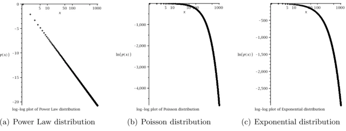
Notice that this distribution is also fat tailed. This means that even for very large k, there is still a fair possibility of there being a vertex of degreek. This distribution does not tend to zero as fast as a Poisson distribution, for example, or an exponential distribution. (See figure 1.1.) Also note that if the average degree of a network is finite, it must hold
γ >2.
It is important to point out that, seeing that real networks are always finite in number, this distribution will have a natural cut-off for an analyzed “real life” network.
x 5 10 50 100 1000 ln p x K20 K15 K10 K5 0
log-log plot of Power Law distribution
(a) Power Law distribution
x 5 10 50 100 1000 ln p x K4,000 K3,000 K2,000 K1,000
log-log plot of Poisson distribution
(b) Poisson distribution x 5 10 50 100 1000 ln p x K2,500 K2,000 K1,500 K1,000 K500
log-log plot of Exponential distribution
(c) Exponential distribution Figure 1.1: Log-Log plots for several distributions for values 1, . . . ,1000.
2 Touching upon Real Networks
2.1 Going from Social Networks . . .
Applying graph theory to the social sciences is not a new concept. Networks of friendships have been investigated since at least the 1920’s [23]. Understanding the structure of human interactions is interesting not only for its own sake, but also the implications of such theories are important: How information spreads, as well as diseases, can be modelled with network theory [37]. While there are several different approaches to social network analysis (for example, see [46, p. 47ff.]), for our purposes, this definition will be sufficient:
Definition 2.1. A Social Network is a set of people or groups of people with some pattern of contacts or interactions between them [38, p. 174].
Among the most fascinating studies concerning social networks are probably the so-called “small-world” experiments conducted by Milgram in 1967. Milgram asked a few hundred random individuals in Omaha, Nebraska, to convey a letter to some target person in Boston, Massachusetts. They were only to pass these letters on to other people they knew on a first name basis. About a quarter of these letters arrived; on average, each letter only passed through six people before arriving at its goal.
Albeit not aiming to prove anything about networks, this experiment later coined the phrase “six degrees of separation,” which is not only the title of a play [25] but also the basic idea behind the small world effect as discussed in subsection 1.3.2.
The classical approach to social networks has some flaws that render it difficult to work with from the point of view of the sciences. First of all, due to the nature of human interactions, it is often necessary to obtain information by directly interviewing people via questionnaires and the like. This is time and cost intensive, and leads to comparatively small sample sizes. The information obtained is often inaccurate, because respondants interpret questions differently. For example, there is no universal definition of the word friend [38, p. 175].
Other methods of analyzing social networks needed to be found; the vast databases now available facilitated research. Investigations of so-called collaboration networks started. A link between two individuals exists here exactly when a trace of their collaboration is in the database.
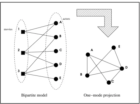
For example, the network of movie actors (nearly half a million people) has been studied with the help of the Internet Movie Database1 [39]. This network can be studied in two ways:
1. As a bipartite graph G(A∪M,E), where there are edges connecting the nodes A
(actors) and the nodes M (movies). There is an edge between ai ∈ A and mj ∈M
iffai has starred in mj
00 00 00 11 11 11 00 00 00 11 11 11 00 00 00 11 11 11 000000000 000000000 000000000 000000000 000000000 111111111 111111111 111111111 111111111 111111111 000000000 000000000 000000000 111111111 111111111 111111111 000000000 000000000 000000000 000000000 000000000 000000000 000000000 000000000 000000000 000000000 000000000 000000000 000000000 000000000 000000000 000000000 111111111 111111111 111111111 111111111 111111111 111111111 111111111 111111111 111111111 111111111 111111111 111111111 111111111 111111111 111111111 111111111 000000000 000000000 111111111 111111111 000000000 000000000 000000000 000000000 000000000 000000000 000000000 000000000 111111111 111111111 111111111 111111111 111111111 111111111 111111111 111111111 000000000 000000000 000000000 000000000 000000000 000000000 000000000 000000000 000000000 000000000 000000000 000000000 000000000 000000000 000000000 000000000 000000000 000000000 000000000 000000000 000000000 111111111 111111111 111111111 111111111 111111111 111111111 111111111 111111111 111111111 111111111 111111111 111111111 111111111 111111111 111111111 111111111 111111111 111111111 111111111 111111111 111111111 000000000 000000000 000000000 000000000 000000000 111111111 111111111 111111111 111111111 111111111 000000000 000000000 000000000 000000000 111111111 111111111 111111111 111111111 000000 000000 000000 000000 000000 000000 000000 000000 000000 000000 000000 000000 000000 000000 000000 000000 111111 111111 111111 111111 111111 111111 111111 111111 111111 111111 111111 111111 111111 111111 111111 111111 0000000000 0000000000 0000000000 0000000000 0000000000 0000000000 0000000000 0000000000 0000000000 1111111111 1111111111 1111111111 1111111111 1111111111 1111111111 1111111111 1111111111 1111111111 0000000000 0000000000 0000000000 0000000000 0000000000 1111111111 1111111111 1111111111 1111111111 1111111111 00000000 00000000 00000000 00000000 00000000 00000000 00000000 00000000 00000000 00000000 00000000 00000000 00000000 00000000 00000000 11111111 11111111 11111111 11111111 11111111 11111111 11111111 11111111 11111111 11111111 11111111 11111111 11111111 11111111 11111111 0000 0000 0000 0000 0000 0000 0000 0000 0000 1111 1111 1111 1111 1111 1111 1111 1111 1111 0000 0000 0000 0000 0000 0000 0000 0000 0000 0000 0000 0000 1111 1111 1111 1111 1111 1111 1111 1111 1111 1111 1111 1111 0 0 0 0 0 0 0 0 0 0 0 0 0 1 1 1 1 1 1 1 1 1 1 1 1 1 0000000000000 0000000000000 0000000000000 0000000000000 0000000000000 0000000000000 0000000000000 0000000000000 1111111111111 1111111111111 1111111111111 1111111111111 1111111111111 1111111111111 1111111111111 1111111111111 2 3 A B C D E 1 actors movies A C D E B
Bipartite model One−mode projection
Figure 2.1: One mode projection
2. As the so-called one-mode projection. where all vertices represent actors, and there is a link between two actors if they have played in a movie together. (See Fig. 2.1.) Note that in the one mode projection, some information is lost. Also, as most films are made with more than two actors, the projection of the vertices obviously causes many triangles, which will influence the clustering coefficient. It is also necessary to point out that even though two actors appeared in the same film, this does not imply that they had any other social contact apart from that; as such, it is questionable if the net of movie actors is representative of human interactions.
2.2 . . . over Scientific Collaboration Networks . . .
The idea behind scientific collaborations is similar. One of the first papers treating this topic from a graph theoretical view was written by Newman who investigated several concepts of complex networks in four vast databases [37].
The concept of investigating scientific collaborations is not completely new, either. In the mathematics community, a very central figure wasPaul Erd˝os (one of the two founders of the theory we will use in chapter 4). He wrote over 1,400 papers during his lifetime, which outnumbers all other mathematicians. In fact, Paul Erd˝os is so central that mathe-maticians started calculating theirErd˝os numbers, which is the distance (via co-authorship of papers) they have to this exceptional scientist. Having co-authored a paper with Paul Erd˝os gives Erd˝os number one, a co-author of someone who has Erd˝os number one has Erd˝os number two, and so on. Erd˝os numbers are so popular that there is an application on the site of the American Mathematical Society2 to calculate the distance between any two mathematicians, with Erd˝os being the default value.
2.2 Scientific Collaboration Networks
medline Los Alamos spires ncstrl
Total papers 2,163,923 98,502 66,652 13,169 Total authors 1,520,251 52,909 56,627 11,994 Mean papers/author 6.4 5.1 11.6 2.55 Mean authors/paper 3.754 2.530 8.96 2.22 Collaborators/author 18.1 9.7 173 3.59 Cutoff zc 5,800 52.9 1,200 10.7 Exponent τ 2.5 1.3 1.03 1.3
Size of giant component 1,395,693 44,337 49,002 6,396
As a percentage 92.6% 85.4% 88.7% 57.2%
Second largest component 49 18 69 42
Mean distance 4.6 5.9 4.0 9.7
Maximum distance 24 20 19 31
Clustering coefficient C 0.066 0.43 0.726 0.496 Table 2.1: Findings from four different networks [37].
As seems natural, in [37] two scientists are linked if they published a paper together. Newman’s data came from medline (papers on biomedical research), the Los Alamos
e-Print Archive (preprints in theoretical physics), spires (papers and preprints in high
energy physics) and ncstrl (preprints in computer science), where he investigated the
papers issued during the five year period 1995–1999.
Newman checked all the essential questions of complex networks. Some of his findings (more sub-cases were investigated) are summarized in table 2.1. On average, authors wrote four papers between 1995 and 1999; each paper has an average of three authors, which slightly biases the clustering coefficient C. Note that the average number of collaborators of an author varies strongly between the different papers. Forncstrl (computer science),
it is below four, while formedlinethe number already rises to 18, reaching 173 forspires.
This can be explained by the nature of the sciences involved: papers published in spires
are by high-energy experimentalists, where many people are involved per paper just to run the experiments.
Newman also tried to fit the number of collaboratorszwith a power-law form, which did not work. However, he succeeded quite well in fitting the data by a power-law form with an exponential cutoff:
P(z)∼z−τe−z/zc
whereτ and zc are constants. One explanation for the cutoff is the finiteness of the data
— only five years of numbers. The values of τ and zc are given in table 2.1, they vary
considerably.
Note that for all these sets of researchers, the giant component of their collaboration graphs comprises more than half of all vertices, in three of them around 90%. This, and the fact that the second largest components are all truly tiny in comparison, show how strongly connected the networks of these scientists are.
They also exhibit the “small-world” property: the average distance between a random pair of vertices is around six. In fact, splitting the data into the different (sub-)groups of scientists, we can see in Fig. 2.2 that this data can be fitted to match the definition of the “small-world” property, as the average distance of two random researchers is plotted
Figure 2.2: Average distance of researchers to average distance in random graph [37] against the average distance in a random graph with the same number of vertices and edges.
These networks exhibit very high clustering coefficients. One explanation is (as with movie actors) that a paper written by three or more authors already induces at least one triangle. However, the values here are so high that this cannot be the only explanation. Interestingly, medline’s clustering coefficient is much lower in comparison. This may be
because of the hierarchical structure of biological laboratories, which could cause tree-like networks without many loops.
Other studies of collaboration networks followed, which have treated new models, for example, see [5]. To summarize Newman’s findings, overall, they fulfilled our expectations which we described in section 1.3. We shall see that collaboration networks are not the only networks that “perform” in this way.
2.3 . . . to the Internet and www . . .
Two of the driving factors in network theory are the internet and the World Wide Web (www). These massive networks are intriguing in their size, fast dynamics and almost com-plete self-organization. Apart from purely scientific reasons, this research is important in applications: web crawls and search engines, network stability questions and understanding the sociology of content creation are only a small number of possible examples [12].
2.3.1 The Internet
First note the difference between the internet and the www [17, p. 34 ff]. The internet is made up of physical components on different levels, such as computers that have activated their connection to the net (hosts), servers that provide service to the web, and routers that arrange traffic across the internet. Edges in this network are the connections between the different components, they are undirected.
2.3 The Internet and www
In the beginning of 2001, it contained about 100 million (108) hosts. Going up one level, we study the internet at the router or interdomain level. Mid 2000 there existed about 150 000 routers in total, a year later there were about 220 000.
Dorogovtsev and Mendes [17] compare several studies of the internet at interdomain level done between 1999 and 2002. At the time, this graph was quite small and sparse; in 1999, it had only n = 5287 vertices, their number and the number of edges connecting them fluctuates considerably. From 1997 to 1999, the average degree increased from 3.42 to 3.8, meaning that connections grow stronger than vertices. The average distance ¯l between two nodes was always below four, and the ratio of ¯l to the equivalent number of the corresponding random graph was 0.6, meaning that the internet shows signs of having the “small-world” effect. The maximum length of separation was around 11, and the clustering coefficient C of 0.2 was considerably higher than that of a classical random graph. The degree distribution manifested a power-law with exponent 2.2.
Note that, because we are talking about physical components here — hardware, cables, and so on — geographical as well as economical influences matter: For example, the fluctu-ations innare due to providers opening or going out of business, while locations of routers etc. have been shown to be closely related to population density.
2.3.2 The World Wide Web
In comparison, the www consists of documents (pages) containing information [11, 17]. When these pages refer to each other, they are connected by hyperlinks. The webpages are the vertices of the web-graph, while the connections are the arcs.
Note that this gives a directed graph. For each page, we are thus looking at links coming in and going out, so we also distinguish in- and out-degrees.
The web is growing quickly [11]. In 1997, there were supposedly 320 million web pages. In 1999, around 800 million were found. A current and accurate estimate is hard to come by, but in 2005 it was stated that the web had about 11.5 billion pages, while shortly after this number was claimed to be 53.7 billion, with 34.7 billion of these pages indexed by Google3.
The directedness of the web changes our definition of the giant component and the way we see the structure of the net. We say the www has abow-tie structure, and we call the giant strongly connected component (GSCC) thecore orknot of the bow. We call vertices connecting to the core part of thegiant in component (GIN) and vertices that have edges connecting from the GSCC part of thegiant out component (GOUT). Note that the GSCC is the intersection of GIN and GOUT. The remaining vertices are either not connected to the giant component, or they are so-called tendrils that connect to the GOUT, or lead away from the GIN. For a schematic view of the (weakly) connected component of the web, see figure 2.3. The connectivity of the web is becoming stronger, as the apparent growth of the core shows: While in 2000, it was estimated that a third of all pages were in the core, a 2006 estimate placed two thirds of all web pages in the GSCC [11].
The first investigation of the web of this size was conducted by Broder, [12], where 200 million pages and 1.5 billion links were examined via the altavista web crawl in 1999. Though the www has grown considerably in the mean time, the first findings remain of interest: Especially the repeated occurrence of power-law distributions is fascinating, as
0000 0000 0000 0000 1111 1111 1111 1111 000 000 000 111 111 111 000 000 000 000 111 111 111 111 0000 0000 0000 0000 1111 1111 1111 1111 0000 0000 0000 0000 1111 1111 1111 1111 000 000 000 111 111 111 000 000 000 111 111 111 000 000 000 111 111 111 0000 0000 1111 11110000 00 00 00 11 11 11 11 11 000 000 000 111 111 111 000 000 000 000 000 000 111 111 111 111 111 111 00000 00000 00000 11111 11111 11111 00000 00000 00000 11111 11111 11111 000000 000000 000000 000000 111111 111111 111111 111111 000000 000000 000000 111111 111111 111111 000000 000000 000000 000000 111111 111111 111111 111111 000000 000000 000000 111111 111111 111111
GSCC
tendrilsGIN
GOUT
tendrils Figure 2.3: GSCC well as the results concerning the giant component.In fact, it was found that the in-degree of the www has a power-law with exponent around two, i.e. pin
k ∼ k21.1, a number already reported in earlier, smaller searches. The out-degree
distribution was also a power-law with exponent 2.72. Interestingly, the distribution of the sizes of the weakly connected components also exhibited a power law, with exponent 2.5.
Treating the www as an undirected graph, 91% (186 million) of all nodes were in the giant (weakly connected) component. This component was shown to be surprisingly robust and well connected: if all edges to pages of degree greater than 5 had been removed, the graph would have still contained a weakly connected component of 59 million vertices. The average undirected distance was shown to be 6.83.
The distribution of the sizes of strongly connected components also exhibits a power law. Broder’s study [12] also found the (directed) diameter of the www to be at least 28, counting only pairs of vertices for which there actually exists a directed path connecting them.
2.4 . . . and Beyond
A myriad of applications can be described by complex networks. In this last section, I will name a few more, and briefly describe some.
One fairly old idea that has been revived lately is the investigation of citation networks, an overview given in [17]. Papers citing other papers form a so-calledcitation graph. In this model, papers are the nodes and citations are the arcs. A new paper links to older papers, and older papers do not change, so they cannot form any new links. When preprints are disregarded, this directed network is acyclic, even though the underlying undirected graph may have cycles. Also note that most empirical surveys of citation graphs measure the current state of the graph, and not how it evolves over time.
In fact, one of the first studies to report a power-law degree distribution P(k) was about citation networks by Redner [42]. He investigated data from the Institute for Scientific Information (ISI database) including 783,339 papers and 6,717,198 citations, and data from Physical Review D (PRD) of 24,296 papers with 351,872 citations.
Redner tried to fit the data with a stretched exponential,
P(k)∼exp −xk 0 β! ,
2.4 Brief Outlook
but this did not explain for the (few, widely scattered) very big values of degreek. For ISI only 64 out of over 700,000 paper are cited more than 1000 times, 282 are cited more than 500 times, while over 300,000 papers are uncited. Redner looked for a function that was less smooth, and showed that the data fitted well toP(k)∼k−α, with α close to 3.
It was later proposed to fit the data with (k+ const)−α, where α= 2.9 for the ISI net, and α = 2.6 for the PRD data, and even later it was stated that the data was still not large enough to be sure that the distribution is really fat-tailed. Different possibilities to fit the data exist, although there is evidence for preferential attachment in the citing process. This would imply a scale-free distribution.
Another science where graph theory has been implied to model “real-world” networks is biology: From directed food webs (arcs indicating who eats whom) to neural networks (There are 100 billion neurons in the human brain, the largest network mentioned in [17].), from metabolic reactions to protein networks (such asprotein-protein-interactions (PPIs)). Some criteria of complex networks (small world effect, etc.) are always present.
Other graphs the theory of complex networks is analyzing are the Word Web of human language, various communication networks (mail networks, the telephone call graph, . . . ) as well as power grid networks, energy landscape networks and many, many more. For a very vivid description of why the latter two are important, see the opening chapter of [46].
3 Methods
In this chapter, a few of the methods, definitions and notations used throughout this diploma thesis are presented. It is divided into three sections:
• Methods used by physicists that a mathematician might not have seen on the core course curriculum,
• a brief refreshment of methods used in probability theory, as well as some theorems that might not be familiar, and
• notations and abbreviations used.
3.1 Methods from Statistical Physics
3.1.1 The Mean Field Method and other Continuum Approaches
The mean field method seems to stem from statistical physics; statistical mechanics, to be exact. Finding an exact definition of the mean field method in general (as opposed to some application of mean field theory to some particular example) has proved difficult.
The basic idea behind is to view a discrete process as a continuous one by considering the same model several times, and then taking the mean of the outcome. This comes from the fact that, when particles are being considered, the mean over time is more relevant than the exact number of particles passing through the investigated area. The same thing is possible when quantities of considerable size are being treated. Quoting from [17]
. . . , master equations become very simple. At first sight, this must work for large degrees, but mathematicians know that such limiting is an extremely dangerous operation. Sometimes it works, sometimes not, and while using the continuum approximation, you have to check your work all the time. However, for simple growing networks this approximation usually yields exact results for most useful quantities or produces unimportant deviations.
This is the reason why, as noted in subsection 1.1.1, there are many heuristic results and rather few rigorous ones — they are easier to find. Most (but not all) have been proved true when rigorous treatment was possible.
3.1.2 The Master Equation
When dealing with Markov chains (see subsection 3.2.3), an important aspect is themaster equation. It gives the rate of change of the probability P(x, t) due to transitions into the
statexfrom all other states and due to transitions out of a statexinto all other states [43], i.e. for a system with npossible states
∂P(x, t) ∂t = n X i=1 ((P(i, t)pi,x(t)−P(x, t)px,i(t)) ,
where pi,j(t)∆t is the probability of a transition from state i to state j during the time
change t→t+ ∆t.
3.2 Methods from Probability Theory
3.2.1 Some Distributions
• We say a random variable X has Poisson distribution,X∼Po(λ) if
P(X =i) = λ
i
i!e
−λ for i= 0,1, . . .; λ >0.
• We say a random variable X has exponential distribution, X ∼ E(x, λ) if for its density function f(x) it holds
f(x) =λe−λx for x >0.
For its distributionF(x), it holdsF(x) = 1−e−λx.
• For a random variable X with Bernoulli distribution with mean p, we will write
X∼Be(p).
• For a random variableXwith binomial distribution with parametersnandp, we will write X∼Bi(n, p). For nk
pk(1−p)n−k we will use the notation Bi(k;n, p).
3.2.2 Two familiar Inequalities
Let us just state these inequalities (both from [28]) again as a reminder to the reader:
Theorem 3.1 (Chebyshev’s inequality). For a random variable X, if Var(X) exists it holds
P(|X−EX| ≥t)≤ Var(X)
t2 , t >0.
Theorem 3.2 (Markov’s Inequality). For a random variableX ≥0almost surely, it holds
P(X≥t)≤ EX
t , t >0.
For a series of random variables Xn we say Xn converges in distribution toZ asn→ ∞
written as Xn→d Z ifP(Xn≤x)→P(Z≤x) for every real x that is a continuity point of
3.2 Methods from Probability Theory
3.2.3 Markov Chains
For a sequence of random variables (xn)n∈N, let{xn} denote the filtration of the sequence
up to time n, i.e. the event that (x0 ∈ X0, x1 ∈ X1, . . . , xn ∈ Xn) for some events
X0, X1, . . . , Xn.
Definition 3.1(Markov Process [29]). Let(Ω,B, µ)be a filtration space with a denumerable stochastic process(xn)n∈N defined fromΩto a denumerable state space S of more than one
element. The process is called a denumerable Markov process if, for any n,
P(xn+1∈cn+1 |x0 ∈c0∩ · · · ∩xn−1 ∈cn−1∩xn∈cn) =P(xn+1∈cn+1 |xn∈cn)
for any states c0, . . . , cn+1 such that P(x0 ∈c0∩ · · · ∩xn−1 ∈cn−1∩xn∈cn)>0.
For a finite, time homogenous Markov process with npossible states, [n] :={1,2, . . . n}, we call the matrixP ∈Rn×n the transition matrix where p
ij is the probability of passing
from stateito state j.
Note that in Pm, the elementp(ijm) gives the probability of passing from stepito step j
inm steps. A state i in a Markov chain is calledergodic if, for every state j it is possible to go fromito j, possibly via several steps. This is equivalent to saying that there exists anm so thatp(ijm) >0 for everyj. A Markov chain that consists of ergodic states is called irreducible.
If there exists a subset of states A⊂[n] such that pij = 0 for every pair (i, j) such that
i∈ A, j ∈ [n]/A, this subset is called an absorbing subset. Once an absorbing subset is reached, it is no longer possible to leave this subset. These subsets are also called essential classes. If a Markov Chain has an absorbing subset of size 1, it is called reducible.
If there are absorbing subsets of a finite Markov process that also has ergodic states, it is always possible to write the transition matrixP in this form:
P = R 0 S′ Q , (3.1)
where R is the square matrice associated with the absorbing states of the process, while
Q is the square matrice associated with the ergodic states. It can be shown that, with probability tending to 1 a process that is not irreducible will end in an absorbing state.
We consider a Markov chain consisting of both ergodic and absorbing states. We denote the set of ergodic states by I. Let us denote the random variable Zij as the number of
visits to statej∈I starting from i∈I, (Zii≥1). Then
Zi =
X
j∈I
Zij, i∈I
is the time to absortion of the chain starting from i∈ I. We denote EZij with mij and
EZi with mi. Let M be the matrix whose entries consist of mij and mthe vector of the
Theorem 3.3 ( [44]). Under the assumptions stated above,
M= (I−Q)−1, (3.2)
m=Me= (I−Q)−1e, (3.3)
where Q is the submatrix of the transition matrix P as defined in (3.1), I is the identity matrix, and eis a vector consisting of ones.
3.2.4 Martingales
Definition 3.2 (Martingale [28]). For a probability space (Ω,F,P) and an increasing se-quence of sub-σ-fields F0 ={∅,Ω} ⊆ F1 ⊆ · · · ⊆ Fn =F, a sequence of random variables
X0, X1, . . . , Xn(with finite expectations) is called a martingaleif for eachk= 0, . . . , n−1,
E(Xk+1 | Fk) =Xk.
Often, Ω is a finite space andF the family of all subsets; Fk corresponds to a partition
Pk of Ω, with finer partitions for largerk. Note that it is also possible to consider sequences
of sub-σ-fields of the form (Fn)n∈N with corresponding sequences of random variables of
the form (Xn)n∈N.
Theorem 3.4 (Azuma-Hoeffding inequality [28]). If (Xk)n0 is a martingale with Xn =X
and X0 =EX, and there exist constants ck>0 such that
|Xk−Xk−1| ≤ck
for each k≤n, then, for everyt >0,
P(X≥EX+t)≤exp − t 2 2Pn k=1c2k , P(X≤EX−t)≤exp − t 2 2Pn k=1c2k .
3.3 Notations and Abbreviations
Throughout this diploma thesis, the following standard notation is used to describe asymp-totics, see i.e. [28]. For a sequence of two numbers, an ∈ R and bn > 0, depending on a
parametern→ ∞, we write
• an = O(bn) as n → ∞ if there are constants C and n0 such that |an| ≤ Cbn for
n≥n0, i.e., the sequence an/bn is bounded forn≥n0.
• an = Ω(bn) as n → ∞if there exist constants c >0 and n0 such that an ≥cbn for
n≥n0.
• an= Θ(bn) as n→ ∞ if there exit constants C, c ≥0 and n0 such that cbn ≤an ≤
Cbn, i.e.anandbnare of thesame order of magnitude. We may also use the notation
an∝bn.
3.3 Notations and Abbreviations
• an=o(bn) as n→ ∞ifan/bn→0.
• an≪bn orbn≫an ifan≥0 and an=o(bn).
Both the abbreviations a.a.s., meaning asymptotically almost surely, as well as whp, meaningwith high probability are used to describe that a propertyEnof a random structure
that depends onnholds withP(En)→1 asn→ ∞. U.a.r. stands for uniformly at random.
For two events E1 and E2, we say that E1 ⊂ E2 if E1 ⇒ E2. We use the notation (n)k:= (nn−!k)!, as well as the notation [n] :={1,2, . . . , n}.
4 The “classical” Random Graph Model by
Erd˝
os and R´
enyi
4.1 The Model
The initial model of random graphs goes back to Erd˝os and R´enyi, see e.g. [22]. There are two essentially equivalent approaches to see random graphs [28], denoted byGn,N and
Gn,p. In both models, we have nlabeled vertices, v1, v2, . . . , vn. Both models are random;
they differ in the way the edges are chosen.
InGn,N,N edges are chosen at random from the n2 possible edges, where each edge is
chosen with equal probability. Out of the (n2)
N
=: Cn,N possible resulting graphs, each
one appears with equal probability, i.e. each resulting GraphGn,N appears with probability
1
Cn,N. This model is called the uniform random graph model. Contrarely, in the model Gn,p each of the n2
possible edges appears with probability 0 ≤ p ≤ 1. Thus, for p = 0 we will have a graph on n vertices containing no edges, i.e.
Gn,0, while forp= 1 we will have Gn,(n
2), the complete graphKn. A graph thus obtained
is also calledbinomial random graph.
To be correct, we should denote byGn,N andGn,p the set of all graphs obtained by the
uniform and binomial random graph models, respectively. However, by abuse of notation, when it is clear with which we are dealing, will refer to both the set of all random graphs as well as a certain graph picked from the set withGn,N and Gn,p.
Definition 4.1. For a given graph G we define the corresponding random graph as a Erd˝os-R´enyi random graph Gn,N withn=|G| andN =|E(G)|.
Another approach concerning Gn,N is the following: Out of the n2
possible edges, we choose at first only one. Then, out of the remaining n2
−1 edges, we chose another one at random, and so forth until we chose ourNthedge out of n2
−N+1. In this model, the inter-est lies in increasingN. This can be seen as a random graph process, which we will denote by (G(n, N))N. LettingN = N(n) and n → ∞, investigations of “typical behavior” are made, depending onN(n). This can mean that if limn→∞Pn,N{Gn,N has propertyQ}= 1,
“almost all” Graphs inGn,N have this characteristic Q.
Several properties of random graphs have been thouroughly examined, questions such as: How large mustN be so that almost all graphs in Gn,N have a cycle of order k? How
many graphs do not have any tree of orderl? If we let An,N denote the number of graphs
ofGn,N having a certain propertyQ, obviouslyPn,N(A) = ACn,Nn,N is the probability that any
chosen graph ofGn,N will haveQ.
Definition 4.2. We define a propertyQ on graphs G=G(V, E), |V|=n, formally in the following way: Q ⊆2(n2), where 2(
n
Intuitively, Gn,p and Gn,N are equivalent; Gn,N can be seen as a random graph {Gn,p :
|E|=N}. Asymptotically, this is in fact so, as the following theorems show [28]. In the rest of this chapter, we will use either Gn,p or Gn,N, depending on which is more convenient.
Note that, even though the notation is the same, it will always be clear from context which model is being treated.
Proposition 4.1. Let Q be a random property of subgraphs of the complete graph Kn a
graph Gmay or may not have, p=p(n)∈[0,1]and 0≤a≤1. If for every sequenceN =
N(n) such thatN = n2
p+Oq n2
pq, whereq = 1−p, it holds thatP(Gn,N ∈ Q)→a
as n→ ∞, then alsoP(Gn,p∈ Q)→a as n→ ∞.
For a proof of this theorem, see [28].
For the other direction no equivalence can be found in such generality. A counterexam-ple is the property of a graph containing exactly N edges. However, with the following definition and lemma, a result can be obtained.
Definition 4.3. A family of subgraphs Q ⊆2Kn is called increasing if A⊆B and A∈ Q imply that B∈ Q. Vice-versa, a family of subgraphs is called decreasing if its complement is increasing. An increasing or decreasing family is called monotone.
Lemma 4.1. Let Q be an increasing property of subgraphs of Kn, 0 ≤p1 ≤p2 ≤ 1 and 0≤N1 ≤N2 ≤ n2 . Then P(Gn,p1 ∈ Q)≤P(Gn,p2 ∈ Q) and P(Gn,N1 ∈ Q)≤P(Gn,N2 ∈ Q).
Proof. For this proof we first apply the so-called two-round exposure technique, which applies to the binomial model, viewing the random graph process GN,p as the union of
two independent random graph processes Gn,p1 and Gn,p2, where the edges of each model
are taken, and double edges are replaced by one edge, for p = p1 +p2 −p1p2. We set
p0 = (p2−p1)/(1−p1). Now, Gn,p2 can be viewed as a union of two independent random
graph processes, Gn,p0 and Gn,p1. Thus, Gn,p1 ⊆ Gn,p2, and with Q increasing, the first
inequality follows, as the event ofGn,p1 ∈ Q impliesGn,p2 ∈ Q.
To prove this lemma for the uniform model, it suffices to construct a random graph process{G(n, N)}N. Gn,N is now theNthprocess in order, and obviously Gn,N1 ⊆Gn,N2.
With the same arguments as in the first part of the proof, the second inequality is shown.
Proposition 4.2. Let Q be a monotone property of subgraphs of Gn, 0 ≤ N ≤ n2, and
0≤a≤1. If for every sequencep=p(n)∈[0,1] such that
p= Nn 2 +O v u u t N n2 −N n 2 3
it holds that P(Gn,p)→a, then P(Gn,N)→a.
4.2 Threshold Functions
4.2 Threshold Functions
For many graph properties E there exist so-called threshold functions [22, 28] which we shall denote byA(n),A(n)→ ∞ forn→ ∞such that
lim n→∞Pn,N(n)(E) = 0 if lim n→∞ N(n) A(n) = 0 1 if lim n→∞ N(n) A(n) = +∞
It can be shown (see [28, page 20]) that every monotone property has a threshold.
The next theorem is a good example of threshold functions; several properties are special cases of following general case. Out of historical interest, the proof is from the original paper by Erd˝os and R´enyi [22]. The same result can be shown much quicker using modern probabilistic tools [28].
Definition 4.4. A graph is said to be balanced if it has no subgraph of strictly larger average degree. This means a graph G(V, E) with |V| = k and |E| = l is balanced if for every subgraph withk′ vertices and l′ edges it holds that l′ ≤k′l/k.
Theorem 4.1. For k, l∈N, k≥2, k−1≤l≤ k2 let Bk,l = n Bk,l1 , . . . , BRk,l:∀i6=j:Bik,l≇Bk,lj o, 1≤R≤ k 2 l ,
be a set of balanced graphs consisting each of k vertices and l edges. Then the threshold function for the property that any random GraphG from Gn,N should contain at least one
subgraph isomorphic to some element ofBk,l is n2−k/l.
Proof. LetPn,N(Bk,l) denote the probability that a random graph ofGn,N contains at least
one subgraph isomorphic to one element of the class Bk,l. There are nk possibilities of
selectingk vertices from which we form a graph in Bk,l (which can be done in R possible
ways). The remainingN −l edges can be selected from the n2
−l other possible edges. (Note that we are counting some graphs more than once.) Thus,
Pn,N(Bk,l)≤ n k R (n 2)−l N−l (n 2) N =O Nl n2l−k .
Assuming thatN =o(n2−k/l), thenP
n,N(Bk,l) =o(1), so there are no subgraphs isomorphic
to a subgraph inBk,l almost sure.
The other direction is a bit longer:
LetBk,l(n):={S ⊆Kn:∃Bk,li ∈ Bk,l:S ∼=Bik,l}. For anyS ∈ B
(n) k,l we define 1(S) := 0 ifS ⊆Gn,N 1 ifS *Gn,N Then it follows X S∈B(k,ln) 1(S) ! = n k R
E X S∈B(k,ln) 1(S) ! = X S∈Bk,l(n) E1(S) = n k R (n 2)−l N−l (n 2) N ∼ R k! (2N)l n2l−k. IfS1∈ Bk,l(n),S2 ∈ Bk,l(n),E(S1)∩E(S2) =∅, then E(1(S1)1(S2)) = (n 2)−2l N−2l (n 2) N .
If |V(S1)∩V(S2)| =s and |E(S1)∩E(S2)| = r, 1 ≤ r ≤ l−1, i.e. S1 and S2 have s mutual vertices andr mutual edges, then
E(1(S1)1(S2)) = (n 2)−2l+r N−2l+r (n 2) N =O N2l−r n4l−2r .
As S1∩S2 ⊆Si,i= 1,2, i.e. a subgraph, and by our supposition everyS is balanced, it
follows rs ≤ kl, sos≥ rkl . At most we then have
R2 k X j=rk l n k k j n−k k−j =On2k−rkl
pairs of such subgraphs. We then obtain
E X S∈Bk,l(n) 1(S) !2 = = X S∈B(k,ln) 1(S) + n!R 2 (k!)2(n−2k)! (n 2)−2l N−2l (n 2) N +O Nl n2l−k 2 l X r=1 n2−k/l N !r! . (4.1)
From the fact that, for C >0,M, N, x∈N,
f(x) = logC M−x N−x = logC M −x M−N
is a concave function, i.e. f(x) +f(y)<2f x+2y
, it follows that n! (k!)2(n−2k)! (n 2)−2l N−2l (n 2) N ≤ n k 2 (n 2)−l N−l 2 (n 2) N 2 .
Note that through this estimate, we have taken into account those possible subgraphs which do not have any common edges but do have possibly one or more common vertices.
We set N
4.2 Threshold Functions
Our next goal is to find an approximation for
Var X S∈Bk,l(n) 1(S) ! =E X S∈B(k,ln) 1(S) !2 − E X S∈B(k,ln) 1(S) !!2 We know that E X S∈B(k,ln) 1(S) !!2 ∼O R k! 2 (2N)2l n2(2l−k) ! =O R2l k! 2 ω2l Also,with (4.1) E X S∈B(k,ln) 1(S) !2 = =O N n2−kl l! +R2 O n k 2 (n 2)−l N−l 2 (n 2) N 2 +O N n2−kl 2l l X r=1 n2−kl N !r! ≃ ≃ R 2 k!2n 2kn−2l2lNl+O(ωl) +O(ω)2l−1 . Thus, Var X S∈B(k,ln) 1(S) ! =O 1 ωE X S∈Bk,l(n) 1(S) 2 !
With Theorem 3.1, it follows
Pn,N X S∈B(k,ln) 1(S) ! − X S∈B(k,ln) E1(S) ! ≥ 12 X S∈Bk,l(n) E1(S) !! =O 1 ω so Pn,N X S∈Bk,l(n) 1(S) ! ≤ 1 2 X S∈Bk,l(n) E1(S) !! =O 1 ω . From ω → ∞,P S∈B(k,ln)E
1(S) → ∞, it follows more than that Gn,N contains at least one
subgraph isomorphic to an element Bi k,l ∈ B
(n)
k,l with probability tending to 1: There will
beO(ωl) many of these isomorphic subgraphs, their number tending to∞. This result has been proved for non-balanced subgraphs as well [7, page 85]. Note that this theorem yields the following interesting results:
• The threshold function for the appearance trees of orderk isnkk−−21.
• ForN ≫n, a random graph will have a cycle of orderk,k∈Nasymptotically almost sure.
4.3 The Giant Component
An intriguing question is the forming of the so-called giant component. That is, asn→ ∞, how strongly mustN → ∞so that a proportion of the vertices ofGn,N is in the largest
con-nected component of the graph, i.e. the size of the largest component is Θ(n). Equivalently, one can investigate how large p(n) must be so thatGn,p forms a giant component.
In 1959, Erd˝os and R´enyi [21] showed that, for N =N(c) =nlogn+cn, the probability that a graph consists of one large connected component (that contains n−k vertices) and
kisolated vertices tends to one, where k=k(n, c). Using this result, they showed that the probability of ofGn,N(c) being completely connected tends to e−e
−2c
forn→ ∞:
Theorem 4.2. Considering Gn,N, where it holds that
N =Nc =
1
2nlogn+cn,
let Pc(n, N) of Gn,N be the probability of Gn,N being completely connected. It then holds
that
lim
n→∞Pc(n, N) =e −e−2c
.
Equivalently, this means that for p ≫ lognn+ 2nc, Gn,p will be connected with the same
probability.
A year later, they published a groundbreaking paper [22], that investigated threshold functions for various properties of random graphs. The results included connectivity char-acteristics whenN(n)∼cnwhich were surprising.
We shall prove that the threshold function for a giant component is at N(n) = n2, which is equivalent to np= 1 forGn,p. A curious aspect here is not only the threshold function,
but also the phase transition from one state into the next. Erd˝os and R´enyi suggested a “double jump” in the size of the largest component, stating it would change fromO(logn) to Θ(n23) and then to Θ(n). In [28, page 111] some evidence can be found against this
statement. For a more detailed description of the phase transition, see [27].
Prior to proving the above statement, we shall need following theorem (Chernoff’s in-equality) [28, page 26]. We will also need some implications of Chebysheff’s inequality. Primarily, we want to show when a random variable will be reasonably close to its mean with high probability. Needing something stronger than Chebysheff’s inequality, we shall use this basic idea which follows from Markov’s inequality (theorem 3.2). For u≥0,t≥0,
P(X≥EX+t) =P(euX ≥eu(EX+t))≤e−u(EX+t)EeuX, (4.2) and vice versa, for u≤0
P(X≤EX−t) =P(euX ≤eu(EX−t))≥e−u(EX−t)EeuX. (4.3) Assuming X is a sum of independent random variables, X =Pn
i=1Xi, with (4.2) we get, foru≥0 P(X ≥EX+t)≤e−u(EX+t) n Y i=1 EeuXi. (4.4)
4.3 The Giant Component
We are especially interested in the case where the Xis are indicator functions, thus
Xi ∼ Be(pi), with pi = P(Xi = 1) = E(Xi). We will denote λ := E(X). (4.4) now
simplifies to
P(X≥EX+t)≤e−u(λ+t)(1−p−peu)u where λ=np. (4.5) Differentiating and setting to zero, we see that the minimum of (4.5) is reached for
eu = (λ+t)(1−p)
p(n−λ−t) for n > λ+t. For (4.4), we get
P(X ≥EX+t)≤ λ λ+t λ+t n−λ n−λ−t n−λ−t for 0≤t≤n−λ. (4.6)
Theorem 4.3 (Chernoff’s inequality). Let X ∼ Bi(n, p) and λ=np. We define ϕ(x) := (1 +x) log(1 +x)−x, x≥ −1, (ϕ(x) =∞ for x <−1) P(X≥EX+t)≤exp −λϕ t λ ≤exp − t 2 2(λ+3t) , t≥0, (4.7) P(X≤EX−t)≤exp −λϕ −t λ ≤exp −t 2 2λ , t≥0 (4.8)
Proof. (4.6) can be written as
P(X≥EX+t)≤exp −λϕ t λ −(n−λ)ϕ −t n−λ , 0≤t≤n−λ. Similarly, by using exactly the same arguments as above for (4.3),
P(X≤EX−t)≤exp −λϕ t λ −(n−λ)ϕ t n−λ , 0≤t≤λ.
For allx, it holds thatϕ(x)≥0, so (4.7) and (4.8) follow directly. Note that we are only interested in the non-trivial cases where 0≤t≤n−λ or 0≤t≤λ.
Asϕ(0) = 0 andϕ′(x) = log(1 +x)≤x, it followsϕ(x)≥x2/2 for −1≤x≤0, so (4.8) is shown.
(4.7) can be seen similarly: ϕ(0) =ϕ′(0) = 0,
ϕ′′(x) = 1 x ≥ 1 (1 + x3)3 = x2 2(1 +x3) ′′
soϕ(x)≥x2/(2(1 +x/3)). The inequality then follows.
Lemma 4.2. Let Xn be a random variable, EXn → ∞ and (EXn)2 ∼E(Xn2). It follows
thatXn>0 a.a.s. and that EXXnn →1. This is equal toP(
Xn
EXn 6∈(1−ε,1 +ε))→0,∀ε >0.
Proof. With (3.1), we have ∀ε >0:
P(|X−EX| ≥εEXn)≤ V
Xn
ε2(EX
n)2
To continue, we shall need a basic understanding of branching processes [26].
We define the following process: At time t = 0Z0 hasY0 children, whereY0 = Z1 is a non-negative random variable in N0.
At t = 1, each of the Y0 children has Yi ≥ 0, i= 1, . . . , Z1, children, where all the Yis
are random variables with the same distribution. Then,Z2=PZi=11 Yi, and more generally
Zk+1 =PZi=1k Yi. This process is called a Galton-Watson process. As soon as there is no
more offspring, the entire process dies out, i.e.Zn= 0 impliesZn+l = 0,l >0. This is called
extinction. Note thatZ0, Z1, . . . form a Markov chain. We assume that the distribution of
Yi does not vary over time.
Let P(Z1 =k) =P(Yi =k) =pk denote the probability that Z1 equals k, which is the probability that an object existing at timethaskchildren at time t+ 1 for k= 0,1,2, . . ., P
pk = 1. We shall need the probability generating function of Yi,f(x) =P∞k=0pkxk for
|x| ≤1, and denote its iterates by
f0(x) =x, f1(x) =f(x), and fn+1(x) =f(fn(x)) , n= 1,2, . . . (4.9)
Note that it follows immediately thatfn+1(x) =fn(f(x)). Also,EZ1 =f′(x)|x=1 =Pkpk.
We shall assume two things:
• ∀k : pk 6= 1 and p0 +p1 < 1. This means that f(x) is strictly convex on the unit interval.
• EZ1 =P∞k=0kpk is finite (and so f′(x) is finite as well).
According to [26], this basic result was already discovered by Watson in 1874:
Theorem 4.4. The generating function of Zn is thenth interate fn(x).
Proof. Let f(n)(x) be the generating function of Zn, n = 0,1,2, . . .. The conditioned
distribution of (Zn+1 |Zn =k) is (f(x))k, k= 0,1,2, . . .. Thus, the generating function
of Zn+1 is f(n+1)(x) = ∞ X k=0 P(Zn=k) (f(x))k =f(n)(f(x)), n= 0,1, . . .
Obviously, f(0) and f0 are equal, so by induction and the fact that fn+1(x) = fn(f(x))
it follows that f(n)(x) =fn(x), n= 1,2, . . . .
The original problem concerning branching processes was the question of the probability of extinction.
Definition 4.5 (Extinction). The event that for the above defined sequence (Zn)n∈N and
a jN >0it holdsZn= 0,∀n≥jN, i.e.Zn= 0for all but a finite number ofn. We denote
the probability of extinction with ρ.
Recall that P(Zn+1 = 0 | Zn = 0) = 1, thus the event (Zn = 0) implies (Zn+1 = 0). Thus,
ρ= lim
4.3 The Giant Component
Theorem 4.5. If µ =EZ1 ≤1, the extinction probability ρ = 1. If µ > 1, then ρ is the unique non-negative solution, ρ <1, of the equation
x=f(x). (4.10)
Proof. By induction, we see that fn(0)<1,n= 0,1, . . ..
Also, combining the fact that (Zn= 0) implies (Zn+1 = 0) and Theorem 4.4, we see that 0 =f0(0)≤f1(0)≤f2(0)≤ · · · ≤ρ= limfn(0). With (4.9) we know fn+1(0) = f(fn(0)),
and limfn(0) = limfn+1(0) =ρ, it followsρ=f(ρ), and thus also 0≤ρ≤1.
If µ≤1, then 1≥f′(1)≥f′(x), 0 ≤x≤1. With help of the mean value theorem, we getf′(ζ)(1−x) =f(1)−f(x), soc(1−x) = 1−f(x) for a constant c <1 and 0≤x <1,
thusf(x)> xfor 0≤x <1, so it follows that ρ= 1.
On the other hand, if µ > 1, then f(x) < x for x = 1−ε, ε > 0 sufficiently small. However, f(0) ≥ 0. It follows that there exists at least one solution for (4.10) in the half-open interval [0,1). With Rolle’s theorem, we know that if there were two solutions,
s0 and t0 with 0 ≤ s0 < t0 < 1, there would exist ξ and η, s0 < ξ < t0 < η < 1 with
f′(ξ) =f′(η) = 1, which is impossible becausef(x) is strictly convex.
Also, limfn(0) cannot be 1: (fn(0))n≥0 is a nondecreasing sequence, while it holds
fn+1(0) = f(fn(0)) < fn(0) if fn(0) is close to (but less than) 1. It follows that ρ is
the the only solution of (4.10).
Before applying this theorem to find the structure of the giant component, let us see these two examples (from [28]).
Example 4.1. LetX∼Po(c). Then the probability generating function is
fX(x) = ∞ X i=0 cixi i! e −c = exp(c(x−1)).
Now, if c >1, with (4.10) and setting y= 1−x we obtain the probability of extinction
ρ= 1−β(c), whereβ =β(c)∈(0,1) is the determined by the equation
β+e−βc= 1 (4.11)
Example 4.2. Let Yn ∼ Bi(n, p), np → c > 1 as n → ∞. The probability generating
function ofYn is fYn(x) = n X i=0 n i xipi(1−p)n−i = (1−p+xp)n, and for every real numberx we have
lim
n→∞fYn(x) = exp(c(x−1)) =fX(x), (4.12)
The probability generating function of Yn tends pointwise to the probability generating
function of X ∼Po(c). This means that for n→ ∞, the probability of extinction ρ(n, c) of a branching process defined byYn converges to 1−β(c) where β is defined by (4.11).
With these preliminaries, we now define the “almost-” branching process we need [28]. We approach the structure ofGn,pin the following way: In the first step of this process, we
pick any vertexv inGn,p, find all its neighborsv1, . . . , vr and then we markvas saturated.
In the second step, we choose v1 and mark it as saturated after finding all its neigh-bors v11, . . . , v1s in V(Gn,p)\ {v, v1, . . . , vr}. We continue this process until there are no
unsaturated vertices left in this component.
If we follow a breadth-first approach during this process — i.e. the vertices closer to vare saturated first — then this process resembles very strongly the branching process. Note that the difference here is that, while we had definedZi =PZj=1i−1Yj, i.e. as a sum of a random
number of random variables, here at each step we only add o
![Figure 2.2: Average distance of researchers to average distance in random graph [37]](https://thumb-us.123doks.com/thumbv2/123dok_us/448725.2552069/16.892.274.659.103.411/figure-average-distance-researchers-average-distance-random-graph.webp)
![Figure 5.1: Figures explaining the small-world model [45]](https://thumb-us.123doks.com/thumbv2/123dok_us/448725.2552069/53.892.114.736.790.1009/figure-figures-explaining-the-small-world-model.webp)