Toward Proactive and Reactive Integration
Amedeo Cesta, Nicola Policella and Riccardo Rasconi
ISTC-CNR
Institute for Cognitive Science and Technology
National Research Council of Italy
{
name.surname
}
@istc.cnr.it
Abstract. In this paper we investigate the integration of off-line and on-line scheduling methodologies: scheduling is in fact a process where the proactive and reactive phases represent a continuum: the task of the scheduler should not be limited to the production of a sequence of activities, as well as the process of controlling schedule execution can-not be exclusively played on the ground of on-line reaction and activity dispatchment. We provide an empirical study which analyzes the mutual interactions among a set of off-line and on-off-line constraint-based scheduling approaches. We devise a set of execution management algorithms, and compare their behavior within an experimental framework which allows to directly assess the consequences of each chosen strategy combination, through simulated schedule executions. A number of interesting results are described, opening new perspectives for future work.
Keywords: Scheduling, Reactivity, Execution
Monitor-ing, Constraint Satisfaction Problem
1
Introduction
As the importance of scheduling problem solving method-ologies is being increasingly acknowledged by non-academic environments, all the aspects that support au-tomation in the synthesis and management of schedules are receiving constant attention. One of the most rele-vant issues regards schedule support at execution time. The dynamism and unpredictability which inherently per-meate real-world application domains, make the ability to cope with unexpected events during the schedule execu-tion phase an absolutely primary concern. For instance, the ability to respond automatically (and efficiently!) to unexpected events that occur during normal job-shop floor operations is considered highly desirable. This aspect is being studied in several scientific communities, such as OR and AI, and the relevance of this specific issue is proved by the recent proliferation of results and surveys [1, 8, 13]. Notwithstanding the relatively recent developments, the problem is still far from being exhausted, and offers much room for investigation.
Traditionally, planning and scheduling communities
have tackled the scheduling problem according to one of the two following mainstreams. On one side, much ef-fort has been put into the development of methodologies producing solutions which are characterized by a certain degree of robustness, therefore retaining the ability to ab-sorb the effects of exogenous events. On the other side, the buffer that protects the solution against possible disrup-tions is inherently limited, and the need to devise mecha-nisms to reactively counteract circumstances that fall be-yond its boundaries, is not eliminated.
The present work introduces a schedule management schema where the off-line and on-line approaches are not mutually exclusive. Scheduling is in fact a process where the proactive and reactive phases represent a continuum: the task of the scheduler should not be limited to the pro-duction of a sequence of activities, as well as the process of controlling schedule executability cannot be exclusively played on the ground of on-line reaction and activity dis-patchment. In fact, regardless the proactive approach em-ployed, a dynamic analysis on the actual behavior of the schedule execution is necessary in order to prove, from the operational standpoint, both the efficacy of the choices made and the soundness of the arguments which led to those choices; as for the second point, merely counting on the effectiveness of schedule adjustments at execution time is prone to fostering myopic decisions which may readily result in a complete schedule disruption.
The paper is organized as follows: section 2 presents a detailed description of the particular problem we tackle for our analysis, section 3 briefly explains the structure of the performed experiments, section 4 contains an analysis of the empirical results, while section 5 presents an interpre-tation of the same results, explaining how the information obtained from this analysis can be used to guide future re-search developments.
2
The Integration Schema
Analyzing how the proactive phase may influence the reac-tive phase at execution time is in our opinion as important as assessing the best schedule production strategy on the base of the schedule’s particular dynamic behavior. The
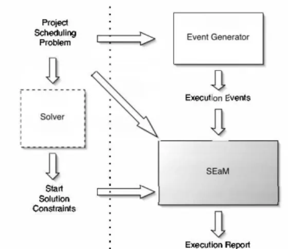
Figure 1: The Integration Schema
information that can be extracted from the two phases may reveal mutually useful in order to find an optimal strategy combination, as well as the reasons behind its optimality.
To this aim, we have devised an experimental plat-form which enables us to compare different approaches to schedule synthesis and execution in a fair and controlled way. We use this empirical platform to carry on a set of experiments by simulating the execution of a number of schedules produced with different proactive methods, dis-turbing their execution with pre-defined exogenous events, and assessing their behavior by using separate reactive scheduling policies. The analysis performed in this paper aims at broadening our understanding of one of the most significant and challenging open problems in the schedul-ing area: unveilschedul-ing the relation between the structural prop-erties of the initial solution and the policies chosen for rescheduling, in terms of overall executional behavior.
The scheduling problem we specifically focus upon is the project scheduling problem [3]. The problems of this class are characterized by a rich inner structure: they are based on a network of activities, among which it is possi-ble to identify complex precedence and temporal relations. As a further source of complexity, several heterogeneous resources with different capacities serve the activities ac-cording to different modalities. In more details the prob-lem is composed of the following eprob-lements
– Activities. A = {a1, . . . , an} represents the set of
activities or tasks. Every activityai is characterized
by a processing timepi;
– Resources. R = {r1, . . . , rm}represents the set of
the resources necessary for the execution of the ac-tivities. Execution of each activityaican require an
amount reqik of one or more resources rk for the
whole processing timepi;
– Constraints. The constraints are rules that limit the possible allocations of the activities. They can be di-vided into (1) temporal constraints which impose
lim-itations on the times the activities can be scheduled at, and (2) resource constraints which limit the max-imum capacity of each resource; at no time, the total demand level of any resource being assigned to one or more activities can exceed its maximum capacity. More specifically, the particular problem we focus upon is the Resource-Constrained Project Scheduling Problem with minimum and maximum time lags, or RCPSP/max
[2]. This is a particular project scheduling problem which presents constraints that define the minimum and maxi-mum distance between the execution of two activities.1
In a recent work [11] we have discussed an approach to the generation of unexpected events to develop reusable benchmarks which could be used to assess the efficacy of re-scheduling policies through reproducible experiments.
According to the schedule management schema we base our analysis upon, the off-line solver produces the initial solution and delivers it to the on-line module which takes care of assessing its dynamic characteristics by simulat-ing its execution under different environmental conditions. Typically these two aspects are carried on as completely separate tasks, and undoubtedly a very high level of spe-cialization and expertise has been reached in both areas: but how useful would it be if the information yielded by one phase could be immediately available to the other? A
prompt analysis of the dynamical characteristics of a par-ticular solution might reveal invaluable to discover possi-ble “weak points” of the off-line solving procedure; con-versely, different reactive strategies might perform more or less efficiently depending on the chosen off-line approach.
Figure 2: The SEaM
In order to fulfill this goal, we have implemented an inte-grated, plug-in based, tool [12] capable of performing both the static and dynamic stages of schedule management. As Fig. 1 shows, it is composed of three modules: the off-line
solver and the Event Generator work off-line and have the
1RCPSP/maxis recognized as a quite complex problem; in fact, even
the feasibility version of the problem is hard. The reason for the NP-hardness lies in the presence of maximum time-lags, which inevitably imply the satisfaction of deadline constraints.
job of, respectively, computing the initial solution and gen-erating the exogenous events intended to disturb the sched-ule execution; the third modsched-ule, called SEaM (for
Sched-ule Execution and Monitoring), is shown in more details
in Fig. 2. This module works on-line and is responsible to start, and possibly bring to completion, a simulated execu-tion of the initial soluexecu-tion. A number of disturbing events synthesized by the Event Generator are injected during the simulated execution at specified times, and their effects are counteracted by the SEaM on-line solver, which is en-dowed with a portfolio of rescheduling algorithms to the aim of restoring schedule consistency whenever necessary. By plugging in different versions of either off-line solvers and/or on-line reschedulers it is possible to explore different aspects of the execution problem. In this paper the experimental framework is organized according to the following general conditions: (a) the solvers are chosen so as to produce initial solutions characterized by differ-ent levels of temporal flexibility; (b) the designated set of rescheduling algorithms shows different levels of repair-ing; (c) the exogenous events produced by the Event
Gen-erator are exclusively of temporal nature (e.g., delays in
the activities start times, lengthenings in the activities du-rations, etc.). In the following paragraphs we describe the previous three points.
Flexible schedules vs. POSs. In contrast to most (off-line) schedulers, which deliver fixed-time solutions, our approach to produce an initial solution, is based on the concept of “temporal flexibility” [6]. A temporally flexible solution can be described as a network of activities whose start times (and end times) are associated with a set of fea-sible values (feasibility intervals). Underlying the activity network there exists a Temporal Constraint Network (TCN [7]), composed of all the start and end points of each ac-tivity (time points), bound to one another through specific values which limit their mutual distances (activity on the arc representation).
The search approaches used in our schema focus on de-cision variables which represent conflicts in the use of the available resources; the solving process proceeds by order-ing pairs of activities until all conflicts in the current prob-lem representation are removed. This approach is usually referred to as Precedence Constraint Posting (PCP [6]), be-cause it revolves around imposing precedence constraints (the solution constraints) on the TCN in order to solve the resource conflicts, rather than fixing rigid values to the start times. In [4] it is shown that though the previous schedule representation inherently provides a certain level of flexi-bility at execution time, it guarantees both a time and re-source consistent solution only if specific values from the feasibility intervals are chosen for the time points, as de-scribed in the following definition:
Definition 1 (Flexible schedule) A flexible schedule for a problemP is a network of activities such that a feasible
solution for the problem is obtained by allocating each ac-tivity at the temporal lower bound allowed by the network.
In order to overcome the limitation imposed by the flexible schedule, i.e. having only one consistent solution, a gener-alization of the TCN produced by a PCP phase is proposed in works such as [4, 10], in which methods for defining a set of feasible schedules are presented. This new represen-tation is called Partial Order Schedule:
Definition 2 (Partial Order Schedule) A Partial Order Schedule (POS) for a problemP is an activity network, such that any possible temporal solution is also a resource-consistent assignment.
APOSis a special case of a flexible solution and it can be obtained by replacing the solution constraints with a new set of constraints that impose a stronger condition on the TCN (chaining constraints). It should be noted that the im-portance of choosing theRCPSP/maxstems from the need to perform a fair comparison between flexible schedules and partial order schedules. In fact, in the absence of max-imum time lags, aPOS always represents an infinite and “complete” set of solutions, as it always allows to avoid a re-scheduling phase (propagating the changes that have occurred is sufficient). In the case of flexible schedules in-stead, propagation alone is not generally sufficient, as any unexpected change might introduce resource conflicts.
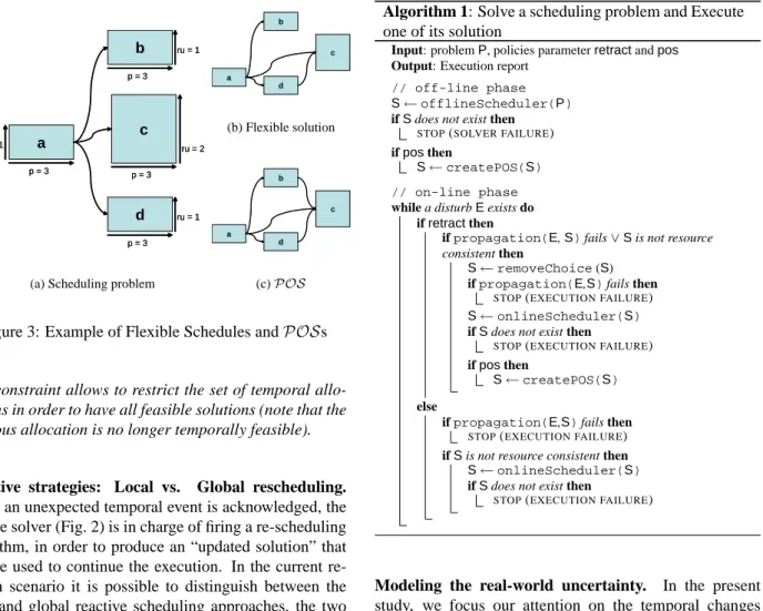
Example 1 Figure 3 shows a flexible and a partial or-der schedule as solutions of a given scheduling problem. Such problem, Fig. 3(a), is composed of four activities, {a, b, c, d}, each characterized by the same processing time,p = 3, and requiring the same resource, character-ized by a maximum capacity = 2: activitiesa, b, drequire one resource unit (ru= 1) and activitycrequires 2 units (ru= 2). Moreover, a set of constraints among the activ-ities further restricts their possible temporal allocations: activitiesb,c, anddcan start only after the complete exe-cution of activitya.
According to Definition 1, a flexible schedule can be ob-tained adding a further precedence constraint betweend andc(see Fig. 3(b)). In fact, by allocating all the activi-ties at their temporal lower bound, we would have thatb,
c, anddare all allocated at the same instant,t = 3, giv-ing an over-requirement on the resource ( 4 units against a maximum availability of 2). Therefore the precedence constraint d ≺ c allows to eliminate this resource peak, returning a feasible solution (the lower bound forcis now att= 6).
According to Definition 2, aPOS requires that all the temporal allocations identified by the activity network be also feasible solutions. This is not the case of Fig. 3(b): in fact, the temporally feasible allocation{0,3,6,4}would not be a resource feasible solution for the problem, be-cause of the violation att= 6. For this reason, aPOSis computed by necessarily adding a further constraintb≺c.
a d c b p = 3 p = 3 p = 3 p = 3 p = 3 p = 3 p = 3 p = 3 ru = 1 ru = 1 ru = 1 ru = 1 ru = 1 ru = 1 ru = 2 ru = 2
(a) Scheduling problem
a d c b (b) Flexible solution a d c b (c)POS
Figure 3: Example of Flexible Schedules andPOSs
This constraint allows to restrict the set of temporal allo-cations in order to have all feasible solutions (note that the previous allocation is no longer temporally feasible).
Reactive strategies: Local vs. Global rescheduling.
When an unexpected temporal event is acknowledged, the on-line solver (Fig. 2) is in charge of firing a re-scheduling algorithm, in order to produce an “updated solution” that will be used to continue the execution. In the current re-search scenario it is possible to distinguish between the local and global reactive scheduling approaches, the two differing by the extension of the revision action’s effects on the initial schedule. In our schema, we model the local and global approach to rescheduling by enabling different constraint removal strategies on the current solution. More specifically:
– No-Retraction strategy: in a local perspective, revi-sions are performed adding further constraints to the current solution (no previously imposed constraints is ever retracted).
– Retraction strategy: in a global perspective, before each revision, all the previously imposed solution or chaining constraints are removed; the subsequent solution is therefore computed by adding new con-straints to this “clean” representation.
In the retraction strategy exceptions are made for the con-straints which model the dynamic aspects of the progress-ing execution: these constraints are always preserved and are used to fix the activities already executed (avoiding to take them into account again in further revisions pro-cesses). The activities not yet executed are allocated again from scratch hence the new solution could be extremely different from the original one.
Algorithm 1: Solve a scheduling problem and Execute
one of its solution
Input: problemP, policies parameterretractandpos
Output: Execution report // off-line phase
S←offlineScheduler(P) ifSdoes not exist then
STOP(SOLVER FAILURE) ifposthen
S←createPOS(S) // on-line phase while a disturbEexists do
ifretractthen
ifpropagation(E,S)fails∨Sis not resource consistent then
S←removeChoice(S) ifpropagation(E,S)fails then
STOP(EXECUTION FAILURE)
S←onlineScheduler(S) ifSdoes not exist then
STOP(EXECUTION FAILURE) ifposthen
S←createPOS(S) else
ifpropagation(E,S)fails then
STOP(EXECUTION FAILURE) ifSis not resource consistent then
S←onlineScheduler(S) ifSdoes not exist then
STOP(EXECUTION FAILURE)
Modeling the real-world uncertainty. In the present study, we focus our attention on the temporal changes which normally characterize the physical environments. In particular, based on the results discussed in [11], we pro-duce a set of exogenous events for every simulated sched-ule execution. For obvious reasons, each set is computed on the basis of the schedule’s initial characteristics. For the present analysis, we consider delays of the activities start times and/or extensions of activity processing times:
– delay of the activity start time: activityai undergoes
a delay of∆sttime units, att=taware;
– increase of activity processing time: ai’s processing
timepiis extended by∆ptime units, att=taware.
For reasons of space we cannot give a complete account on the event generation here. The reader should refer to [11] for further details.
3
Tweaking Proactiveness and Reactiveness
Algorithm 1 illustrates a particular instantiation of our in-tegrated framework, realized with the scheduling technol-ogy described in the previous section. The system imple-ments an “all-round” schedule management architecture, which allows to follow the schedule’s behavior along its complete lifespan. Moreover, it enables the researcher to
combine different strategies and to immediately assess the pros and cons of each chosen option.
In order to distinguish among all the different execution combinations, the algorithm is driven by two flags:
– the flagposallows to distinguish the case in which a POSis created (case POS), from the case in which a flexible schedule is used (case FS);
– the flagretractallows to distinguish between the Retraction strategy (case R from “Retract”) and the No-Retraction strategy case (NR).
From this distinction we globally recognize the four com-binations that are compared in the experimental analysis: FS-NR, FS-R, POS-NR and POS-R. In particular, to pro-duce flexible schedules we have used theISES algorithm [5], because of its efficiency on solvingRCPSP/max prob-lems.POSs creation (createPOS) is instead performed by applying theCHAININGprocedure introduced in [10] to the flexible schedules previously obtained withISES.
For the on-line phase, we slightly modified the previous procedures to obtain computationally lighter versions. In fact, the original procedures, being both based on an iter-ative schema, are CPU expensive: the modified versions are therefore implemented so as to stop the computation as soon as a first viable solution is found, in order to reduce the computational effort. As we will observe in the fol-lowing section, the on-line versions of the algorithms will exhibit the tendency to spoil the initial solution quality.
Finally, in order to further clarify the algorithm, two more points should be remarked: (a) regardless the type of schedule considered (flexible or partial order), the on-line phase of the algorithm is always initiated with the earli-est start time solution; (b) thepropagation()function represents a call to the temporal propagation on the TCN.
The Experiment. In this set of experiments we perform the assessment on off-line and on-line phase combina-tions, by measuring the execution performances in terms of number of successful executions, number of necessary reschedulings, differences in the final makespan, etc.
The comparison presented in this section is based on the analysis of eight different combinations, each obtained coupling two scheduling problem benchmarks, j30 and j100[9], with four reactive scheduling benchmarks. The former consist of two sets of respectively 270 and 540 scheduling problem instances of different size, namely
30×5 and 100×5 (number of activities× number of resources). On the other side, each instance of the reac-tive scheduling benchmark is composed of a set of properly modeled disturbing events (each set representing a “world simulation”). Each problem belonging to the scheduling benchmark2 is executed with four instances of world
sim-2Not all the problems belonging to the scheduling benchmark admit a
solution; moreover,ISESdoes not perform a systematic search. For these reasons, our experimental analysis will necessarily be based on the subset of initially solved problems: 184 forj30and 480 forj100.
ulations of different size (1, 2, 3, and 5 events each).3Each event represents either a delay on the start time, or a delay on the end time of the activities. These two different kinds of event are produced with the same probability.
4
Results Analysis
The results we present in this section emphasize several interesting features about the integration of proactive and reactive phases (Tables 1 and 2). Some results confirm the expectations while others require a certain level of analy-sis in order to be correctly understood. For instance, the behavior of schedules characterized by a more flexible na-ture is totally confirmed. However, the scarce capability in accepting exogenous events which afflicts thePOS was not so predictable, and would not have been revealed with-out a proper testing. The experiments shed light on many possible trade-offs that must be faced, depending on the conditions of execution as well as on the particular as-pects that must be privileged. If fast responsiveness is a primary concern, thePOS is extremely efficient because it rarely needs rescheduling, as opposed to flexible sched-ules. The price to pay for this ability is a higher chance that the event is not accepted by the TCN underlying the problem. Moreover, if solution stability is important, the experiments show that the POS is to be preferred, as it naturally maintains a higher level of solution continuity.
Tables 1 and 2 show the results of our investigation for the FS-R, POS-R, FS-NR, and POS-NR execution strategy. It is worth noting the different nature of the two tables: the first highlights the efficiency of the different methods while the other shows the quality of the solutions found (and for this reason is computed on the intersection set of all successfully executed problems). Again, to make the comparison more complete, we consider also fixed time solutions, where each activity is assigned to a single start time instead of a set of alternatives.
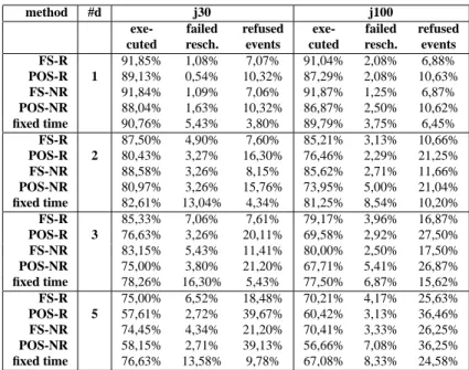
Methods efficiency. Table 1 contains important informa-tion about the number of successfully terminated execu-tions (executed) for every strategy, as well as the reason for failure: the failed resch. column counts the cases where the execution fails because the on-line solver does not succeed in finding an alternative solution; the refused events col-umn counts the cases where the execution fails because the exogenous events are refused due to a constraint violation in the TCN (see section 2). Column #d partitions the table in terms of number of disturbs injected in every execution. The most immediate (and somehow surprising) effect that the dynamic analysis reveals is the POS-R/POS-NR
3The execution of a project scheduling problem can not be considered
completed until all the activities are successfully processed: this implies that any variation is likely to require the synthesis of a new schedule. This represents a major difference with respect to other dynamic problems where the execution of certain activities can be overruled.
method #d j30 j100
exe- failed refused exe- failed refused cuted resch. events cuted resch. events
FS-R 91,85% 1,08% 7,07% 91,04% 2,08% 6,88% POS-R 1 89,13% 0,54% 10,32% 87,29% 2,08% 10,63% FS-NR 91,84% 1,09% 7,06% 91,87% 1,25% 6,87% POS-NR 88,04% 1,63% 10,32% 86,87% 2,50% 10,62% fixed time 90,76% 5,43% 3,80% 89,79% 3,75% 6,45% FS-R 87,50% 4,90% 7,60% 85,21% 3,13% 10,66% POS-R 2 80,43% 3,27% 16,30% 76,46% 2,29% 21,25% FS-NR 88,58% 3,26% 8,15% 85,62% 2,71% 11,66% POS-NR 80,97% 3,26% 15,76% 73,95% 5,00% 21,04% fixed time 82,61% 13,04% 4,34% 81,25% 8,54% 10,20% FS-R 85,33% 7,06% 7,61% 79,17% 3,96% 16,87% POS-R 3 76,63% 3,26% 20,11% 69,58% 2,92% 27,50% FS-NR 83,15% 5,43% 11,41% 80,00% 2,50% 17,50% POS-NR 75,00% 3,80% 21,20% 67,71% 5,41% 26,87% fixed time 78,26% 16,30% 5,43% 77,50% 6,87% 15,62% FS-R 75,00% 6,52% 18,48% 70,21% 4,17% 25,63% POS-R 5 57,61% 2,72% 39,67% 60,42% 3,13% 36,46% FS-NR 74,45% 4,34% 21,20% 70,41% 3,33% 26,25% POS-NR 58,15% 2,71% 39,13% 56,66% 7,08% 36,25% fixed time 76,63% 13,58% 9,78% 67,08% 8,33% 24,58%
Table 1: Success rate of each execution strategy
significantly lower success rate in terms of completed exe-cutions, with respect to all other methods. As shown in the table, the reason lies in a dramatic increase in the number of rejected disturbs (refused events column). This apparent anomaly can be explained in terms of TCN “constrained-ness”: in fact, the creation of aPOS inherently requires a higher number of temporal constraints with respect to a flexible schedule, in order to guarantee a resource conflict-free solution. This inevitably makes the TCN more reluc-tant to accept new disturbing events during the execution phase; this explanation is supported by the worsening of the same effect as the number of events increases.
As readily observable, the case which exhibits the high-est rate of unsuccessful reschedulings is the execution of
fixed time solutions. This is due to the fact that a fixed time
solution requires a rescheduling for every disturbing event, highly stressing the on-line scheduler (which in our case performs an incomplete search), and therefore increasing the possibility of failure. Again, it can be seen that the more events are injected, the more evident the effect.
Solutions qualities. Table 2 presents a different set of results: for each execution policy, it shows the average makespan at the end of every execution (mk), the average difference between the makespan at the beginning and at the end of every execution (∆mk), the percentage of
per-formed reschedulings computed as the ratio between the number of reschedulings and the number of injected dis-turbs (reschedulings), the average CPU time necessary to compute the initial schedule (CPU off-line), and finally, the average CPU time which is necessary to perform all the reschedulings during the execution (all CPU times are ex-pressed in milliseconds). For a fair comparison of the dif-ferent policies, all the averages presented in this table are
computed on the basis of the problem instances commonly executed with all the execution strategies.
One of the most important characteristic to be observed is the extremely low rate of necessary reschedulings exhib-ited by the POS-R/POS-NR policies: this result is all but surprising and confirms the theoretical expectations which motivated the study on thePOS. As shown, the need for schedule revision in case ofPOS utilization roughly de-creases by more than 75% in case of the j30 set, and by at least 50% in case of the j100 set with 5 disturbs. Note also the≈100%reschedulings figure relative to the case
of fixed time schedules: in this case, a schedule revision is almost always needed: this is confirmed by the extremely high CPU on-line values, especially for the j100 set. More-over, the fixed time strategy reveals the highest rates of makespan elongation (see mk and∆mk): in fact, the
fre-quent rescheduling actions, being performed by a less spe-cialized makespan-optimizing procedure to speed up re-action (onlineSchedulerin Algorithm 1), inevitably tend to spoil makespan quality.
A delicate issue should be raised at this point, in order to acquire a better understanding of the presented results: in many scheduling contexts, solution continuity is a funda-mental issue. In our experiments we try to maintain sched-ule continuity through the NR technique, by guaranteeing that every new solution is as close as possible to the pre-vious one, in terms of preservation of the mutual positions among the activities. Moreover, it is clear that continu-ity preservation and makespan optimization are generally conflicting objectives: after the occurrence of exogenous events, the possibility to perform a complete re-shuffling of the activities pays off in terms of makespan minimization, but at the price of a severe continuity disruption. These ob-servations seem to be conflicting with some of the results
method #d j30 j100
mk ∆mk resche- CPU CPU mk ∆mk resche- CPU CPU
dulings off-line on-line dulings off-line on-line FS-R 103.43 4.29 27.27% 4478.31 77.34 424.60 9.02 24.38% 25599.11 766.15 POS-R 1 102.63 3.60 5.19% 4613.57 15.13 419.88 5.07 11.58% 27287.57 303.97 FS-NR 102.56 3.43 27.27% 4481.10 14.68 419.06 3.48 24.14% 25242.48 130.74 POS-NR 102.14 3.10 5.19% 4612.60 2.34 417.11 2.31 11.58% 27251.86 54.59 fixed time 106.29 7.16 100.00% 4480.00 300.45 437.36 21.78 99.75% 25538.68 3035.68 FS-R 106.99 8.02 34.21% 4106.09 150.53 435.54 13.95 23.04% 25347.49 874.70 POS-R 2 104.91 6.03 4.51% 4242.03 20.23 429.22 8.41 10.03% 27529.15 674.86 FS-NR 104.90 5.93 34.21% 4104.89 34.51 427.90 6.30 22.88% 25271.00 258.50 POS-NR 104.83 5.95 4.51% 4239.40 3.83 424.74 3.93 9.56% 27371.82 97.46 fixed time 107.35 8.38 100.00% 4108.80 500.98 446.62 25.02 99.53% 25259.15 2768.37 FS-R 109.55 9.73 26.90% 4506.40 190.00 449.84 19.40 20.27% 25393.55 963.16 POS-R 3 108.11 8.36 5.85% 4647.54 37.02 441.49 11.93 9.41% 27716.81 675.18 FS-NR 108.00 8.18 26.61% 4515.44 39.91 439.66 9.23 22.37% 25318.37 371.03 POS-NR 107.83 8.09 5.85% 4646.23 7.72 436.24 6.68 9.63% 27406.98 151.26 fixed time 109.95 10.12 100.00% 4511.93 848.42 458.32 27.89 99.22% 25300.50 3716.15 FS-R 119.30 16.19 26.43% 4281.90 267.38 464.12 28.85 22.45% 25792.36 2391.92 POS-R 5 116.44 13.37 5.24% 4413.81 73.33 455.56 21.07 10.57% 27162.71 1748.56 FS-NR 117.12 14.01 22.86% 4277.38 59.52 447.42 12.15 21.66% 25682.40 646.90 POS-NR 115.86 12.79 5.00% 4410.60 12.14 444.68 10.18 10.48% 27544.98 289.17 fixed time 118.33 15.23 100.00% 4286.19 1161.19 465.56 30.29 98.43% 25754.32 6721.48
Table 2: Summarizing data (computed on the intersection set of all successfully executed problems)
we present: for instance, one would expect the R strate-gies (which allow a greater re-shuffling) to return better makespan values with respect to NR strategies. Indeed, this is exactly what would happen if we decided to give up reaction times and utilize the same algorithm for both off-line and on-off-line scheduling (as other experiments confirm); but in the present analysis, such expectations are frustrated because the on-line scheduling algorithm severely spoils the makespan of the initial schedule.
Another interesting aspect is related to the comparison of the CPU on-line values (in ms.) between the
Retrac-tion and No-RetracRetrac-tion strategies: in fact, it should be
no-ticed that NR strategies reveal lower CPU-load rates with respect to the R strategies, despite the comparable amount
of performed reschedulings. As explained in section 2, NR
execution modes retain all the temporal constraints of the previous solution: hence, the rescheduler is bound to work on a smaller search space, finding the next solution almost immediately. Additionally, it should be noticed the tremen-dous on-line CPU load in the case of fixed time solutions, as well as how the reactiveness of NR technique, combined with the low revision requirements featured by thePOS, allows for the fastest dynamic reactions of the whole set (see the CPU on-line values for POS-NR).
5
Conclusions and Future Work
Our work is based on the assumption that scheduling is a process where the proactive and reactive phases repre-sent a continuum. In particular this paper introduces a schedule management schema where the off-line and on-line approaches are not mutually exclusive. This schema allows to have a more informed evaluation focusing the at-tention on the combination of off-line/on-line scheduling
techniques.
As shown in the preceding sections, several interesting features are in fact emphasized by this integrated evalua-tion of proactive and reactive phases. Some results confirm the expectations while others require a certain level of anal-ysis in order to be correctly understood. For instance, the rigid behavior exhibited by the fixed time schedules when confronted with dynamically variable environments is to-tally confirmed, as confirmed is the behavior of schedules characterized by a more flexible nature.
However, the scarce capability in accepting exogenous events which afflicts thePOSwas not so predictable, and would not have been revealed without a proper testing. The experiments shed light on many possible trade-offs that must be faced, depending on the conditions of execution as well as on the particular aspects that must be privileged. If fast responsiveness is a primary concern, the POS is extremely efficient because it rarely needs rescheduling, as opposed to flexible schedules. The price to pay for this ability is a higher chance that the event is not accepted by the TCN underlying the problem. Moreover, if solution stability is important, the experiments show that thePOS is to be preferred, as it naturally maintains a higher level of continuity.
The results of this integrated evaluation suggest several research lines which are the object of ongoing work, such as the production of a different class of POSs, through the development of alternative chaining procedures aimed at minimizing the inevitable increase of constrainedness in the TCN, followed by the same on-line experimentation; the latter being necessary in order to highlight possible un-desired side-effects.
As another example, the observed dynamic behavior of the schedules suggests to study the introduction of different
reactive techniques. For instance, a possible approach may be based on informed retraction procedures, where the constraint removal strategy is preceded by a search phase to determine the constraints which are to be retracted, de-pending on the particular dynamic requirements.
Acknowledgments
Amedeo Cesta, Nicola Policella and Riccardo Rasconi’s work is partially supported by MIUR (Italian Ministry for Education, University and Research) under project ROBO -CARE(L. 449/97) and contract #2005-015491 (PRIN).
References
[1] H. Aytug, M. A. Lawley, K. N. McKay, S. Mohan, and R. M. Uzsoy. Executing production schedules in the face of uncertainties: A review and some fu-ture directions. European Journal of Operational
Re-search, 165(1):86–110, 2005.
[2] M. Bartusch, R. H. Mohring, and F. J. Raderma-cher. Scheduling project networks with resource con-straints and time windows. Annals of Operations
Re-search, 16:201–240, 1988.
[3] P. Brucker, A. Drexl, R. Mohring, K. Neumann, and E. Pesch. Resource-Constrained Project Scheduling: Notation, Classification, Models, and Methods.
Eu-ropean Journal of Operational Research, 112:3–41,
1999.
[4] A. Cesta, A. Oddi, and S. F. Smith. Profile Based Algorithms to Solve Multiple Capacitated Metric Scheduling Problems. In Proceedings of the 4th
Int’l Conf. on Artificial Intelligence Planning Sys-tems, AIPS-98, pages 214–223, 1998.
[5] A. Cesta, A. Oddi, and S. F. Smith. An Iterative Sam-pling Procedure for Resource Constrained Project Scheduling with Time Windows. In Proceedings of
the 16th Int’l Joint Conf. on Artificial Intelligence, IJCAI’99, pages 1022–1029, 1999.
[6] C. Cheng and S. F. Smith. Generating Feasible Schedules under Complex Metric Constraints. In
Proceedings of the12thNational Conf. on Artificial
Intelligence, AAAI-94, pages 1086–1091, 1994.
[7] R. Dechter, I. Meiri, and J. Pearl. Temporal constraint networks. Artificial Intelligence, 49:61–95, 1991. [8] W. Herroelen and R. Leus. Robust and reactive
project scheduling: a review and classification of pro-cedures. International Journal of Production Re-search, 42(8):1599–1620, July 2004.
[9] R. Kolisch, C. Schwindt, and A. Sprecher. Bench-mark Instances for Project Scheduling Problems. In J. Weglarz, editor, Project Scheduling - Recent
Mod-els, Algorithms and Applications, pages 197–212.
Kluwer Academic Publishers, Boston, 1998. [10] N. Policella, A. Oddi, S. F. Smith, and A. Cesta.
Gen-erating Robust Partial Order Schedules. In 10thInt’l Conf. on Principles and Practice of Constraint Pro-gramming, CP 2004, LNCS 3258, pages 496–511,
2004.
[11] N. Policella and R. Rasconi. Designing a Testset Generator for Reactive Scheduling. Intelligenza
Ar-tificiale, 3:29–36, 2005.
[12] R. Rasconi, N. Policella, and A. Cesta. SEaM: An-alyzing Schedule Executability through Simulation. In The 19th Int’l Conf. on Industrial, Engineering & Other Applications of Applied Intelligent Systems, IEA/AIE’06, LNAI 4031, pages 410–420, 2006.
[13] G. Verfaillie and N. Jussien. Constraint solving in un-certain and dynamic environments – a survey.
Con-straints, 10(3):253–281, 2005.
Amedeo Cesta (AI*IA Member) is a Senior
Research Scientist for the National Research Council of Italy. His main research areas cover Planning & Scheduling, Multi-agent Systems as well as Human-Computer Interaction. He is particularly interested in filling the gap between theory and practice with AI technology.
Nicola Policella is a Postdoctoral fellow at
the ISTC-CNR. He received a Master degree and a PhD in Computer Science Engineering from the University of Rome “La Sapienza” in 2001 and 2005 respectively. In 2001, he was awarded the AI*IA prize for the best Master Thesis in AI. His current research interests in-clude Scheduling with Uncertainty, Temporal and Resources Reasoning, and Constraint Pro-gramming.
Riccardo Rasconi is a PhD student in
Informa-tion and CommunicaInforma-tion Technologies at the University of Genoa, a research fellow at the ISTC-CNR, and a AI*IA member. His re-search topics are focused on Reactive Schedul-ing, Temporal and Resource ReasonSchedul-ing, and Pervasive Computing.