JOURNAL OF GEOPHYSICAL RESEARCHJGR-Atmospheres
An
Ensemble Version of the E-OBS Temperature and
Precipitation Datasets
Richard C. Cornes1,2, Gerard van der Schrier1, Else J.M. van den Besselaar1 and Philip D. Jones2,3
Richard Cornes, [email protected]
1Royal Netherlands Meteorological Institute (KNMI), De Bilt, Netherlands
2Climatic Research Unit, University of East Anglia, Norwich, United Kingdom
3Center of Excellence for Climate Change Research and Department of Meteorology, King Abdulaziz University, Jeddah, Saudi Arabia
This article has been accepted for publication and undergone full peer review but has not been through the copyediting, typesetting, pagination and proofreading process, which may lead to differences be-tween this version and the Version of Record. Please cite this article as doi: 10.1029/2017JD028200
Abstract. We describe the construction of a new version of the Europe-wide E-OBS temperature (daily minimum, mean and maximum values) and precipitation dataset. This version provides an improved estimation of in-terpolation uncertainty through the calculation of a 100-member ensemble of realizations of each daily field. The dataset covers the period back to 1950,
and provides gridded fields at a spacing of 0.25◦ x 0.25◦ in regular latitude/longitude coordinates. As with the original E-OBS dataset, the ensemble version is based on the station series collated as part of the ECA&D initiative. Station den-sity varies significantly over the domain, and over time, and a reliable esti-mation of interpolation uncertainty in the gridded fields is therefore impor-tant for users of the dataset. The uncertainty quantified by the ensemble dataset is more realistic than the uncertainty estimates in the original version,
al-though uncertainty is still underestimated in data-sparse regions. The new dataset is compared against the earlier version of E-OBS and against regional gridded datasets produced by a selection of National Meteorological Services (NMSs). In terms of both climatological averages and extreme values, the new version of E-OBS is broadly comparable to the earlier version. Nonethe-less, users will notice differences between the two E-OBS versions, especially for precipitation, which arises from the different gridding method used.
Keypoints:
• An improved uncertainty estimate is provided through the generation of multiple realizations
1. Introduction
Gridded datasets formed from the interpolation of station-derived meteorological obser-vations remain a principal source of information for monitoring the climate system. While global, monthly and often anomaly-based datasets provide information about large-scale forcing of the climate, datasets that resolve synoptic-to-meso-scale processes through the provision of daily values at a relatively fine spatial resolution are vital for many ap-plications, especially those involving extremes. Such datasets require a high density of stations — especially when gridding precipitation — and are generally only produced for individual countries due to restrictions concerning the full sharing of daily meteorological observations. Nonetheless, several initiatives have constructed high-resolution datasets for larger regions through the cooperation of National Meteorological Services (NMSs) across neighbouring countries [e.g. Isotta et al., 2014, for the European Alpine region]. However, high-spatial resolution daily gridded data that cover continental regions in a consistent manner are required by many users and it is in this context that the E-OBS dataset was developed for Europe [Haylock et al., 2008].
E-OBS originally consisted of daily mean, minimum and maximum temperature values, and daily precipitation totals gridded at a resolution of ca. 25km and was developed to provide validation for the suite of Europe-wide climate model simulations produced as part of the EU ENSEMBLES project [Hofstra et al., 2008]. In later work Mean Sea-Level Pressure (MSLP) was added as a gridded variable [van den Besselaar et al., 2011]. While E-OBS remains an important dataset for model validation [Nikulin et al., 2011;
climate across Europe [van der Schrier et al., 2013;van Oldenborgh et al., 2016; Lavaysse
et al., 2017], particularly with regard to the assessment of the magnitude and frequency
of daily extremes.
In recent years several regional reanalysis datasets have become available that provide high-resolution, sub-daily datasets for the European domain. These reanalyses have drawn upon the experience gained in the generation of global-scale reanalyses and have retained many of the desirable properties of their global counterparts through the provision of a range of meteorological variables in a consistent manner, for both the surface and at intervals throughout the vertical atmospheric profile. For Europe significant progress has been made in the development of regional reanalysis datasets in two European Union sev-enth Framework Programme (EU FP7) projects: ‘European Reanalyses and Observations for Monitoring’ (EURO4M) and ‘Uncertainties in Ensembles of Regional Re-Analyses (UERRA)’ [Jermey and Renshaw, 2016]. In contrast to global-scale reanalyses, regional reanalyses are able to resolve meteorological processes at a much finer scale and solve many of the limitations of station-based gridding exercises with respect to providing spa-tial and temporal generalizations of climate fields. However, while regional reanalysis datasets have shown great potential, the computing resources required to produce such datasets are considerable, and this has meant that the reanalyses can, in practice, only currently generate data for the last∼20 years. Furthermore, regional reanalyses still show large systematic errors [Isotta et al., 2015;Dahlgren et al., 2016;Bach et al., 2016], partic-ularly for precipitation since rain-gauge data are not currently assimilated into reanalysis datasets. Hence Europe-wide datasets, such as E-OBS, that are relatively quick to pro-duce and which stretch back over longer time periods, remain important tools for climate
monitoring and model validation. Indeed, much of the work described in this paper was carried out as part of the UERRA project, with the aim of providing a more consistent dataset against which the reanalysis datasets constructed during the project could be evaluated. This evaluation role of E-OBS will remain important for the ERA5 global reanalysis, which is currently in production and will ultimately provide a high-resolution (31km) dataset back to 1950.
In this paper we describe and evaluate a new interpolation method for the E-OBS temperature and precipitation dataset. A particular focus in this study is the provision of a better estimate of uncertainty of the gridded data through the generation of an ensemble of daily realizations. Few gridded climate datasets provide estimates of uncertainty, with even fewer estimating this value from an ensemble of realizations. Notable exceptions are the works ofClark et al. [2006] andNewman et al.[2015] (who created ensemble datasets for a region of western Colorado and for the conterminous US respectively), the global HadCRUT4 dataset [Morice et al., 2012] and the gridded dataset for Finland constructed
byAalto et al.[2016]. In addition to the more rigorous estimation of uncertainty afforded
by such ensemble datasets [Beguer´ıa et al., 2016], they also allow uncertainty estimates to be propagated through derived products, such as extremes indices.
The interpolation method described in this paper marks a major departure from the method used in the current operational version of E-OBS, as documented by Haylock
et al. [2008]. In the following section we describe the station data used in the dataset,
and particularly how the density of stations has changed with successive versions of E-OBS. The technique used to calculate the ensemble is also described in that section. In Section 3 the quality of the interpolation is assessed against a selection of withheld station
data, against the current operational version of E-OBS (v16.0) and against a selection of national/supra-national gridded datasets produced by NMSs across Europe. Throughout this paper the term ‘v16.0e’ is used to denote the ensemble dataset, while ‘v16.0’ refers to the current operational version. The variables maximum, minimum and mean daily temperature are referred to as ‘tx’, ‘tn’ and ‘tg’ respectively; ‘rr’ is used to denote the daily total of precipitation variable.
2. The Station Data and Gridding Method 2.1. The Underlying Station Data
The station data collated by the ECA&D initiative [Klein Tank et al., 2002; Klok and
Klein Tank, 2009] form the basis of E-OBS. These data are supplied by many NMSs and
other providers across Europe and the Middle East, although due to restrictions concern-ing the exchange of data the number of stations available to E-OBS is generally lower than the total number potentially available, or the number that is used in most national/supra-national gridded datasets. Although most station series are quality-controlled by the re-spective agencies, the series are subjected to a further quality-control procedure following incorporation into ECA&D. These data are then blended with neighbouring series to form more temporally complete series [van der Schrier et al., 2013; The ECA&D Team, 2012] and these blended series are used in E-OBS. To update the series to near real-time, data are used from synoptic messages (SYNOP) distributed via the Global Telecommunications System (GTS). The SYNOP data are replaced when validated data become available from the NMSs but these validated series are often delayed due to the data being subjected to additional quality-control procedures by the respective agencies [van den Besselaar et al., 2012]. A range of different methods are used to calculate the daily values, and this is often
dependent upon the convention used by a given data provider. For example, daily mean temperatures may be the average of maximum and minimum temperatures, or may be the average of hourly readings, or another frequency such as three-hourly. This variation is not accounted for in the gridding of the data. Furthermore, uncertainties in the measure-ment of the variables are not taken into account in the gridding, or in the ensemble-based uncertainty estimates, which only quantify interpolation uncertainty. While such errors are likely to be present in both the temperature and precipitation data, measurement errors in precipitation may be substantial, particularly at high-elevation or high-latitude stations [Neff, 1977;Legates and Willmott, 1990;Yang et al., 1999a].
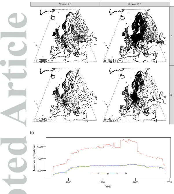
Since the initial construction of E-OBS by Haylock et al. [2008] many more station series have been added to ECA&D (Figure 1a), with an increase from ca. 1200 to ca. 3700 stations for temperature, and from ca. 2500 to ca. 9000 stations in the case of precipitation. However, since only certain agencies have increased the number of stations in ECA&D, there has been an increasing disparity in station density across the domain, with relatively many stations across central Europe and Scandinavia, and many fewer towards the south and east of the domain. It should also be noted that many more stations are available in ECA&D east of 50◦E but since these are not incorporated into E-OBS they are not plotted in Figure 1a. In addition to the highly variable station-density, the number of stations available for gridding also varies significantly over time with many fewer stations before ca. 1961 and a decrease in density after ca. 2000; this has been a deficiency in E-OBS since its inception (Figure 1 b, c.f. Figure 2 inHaylock et al.[2008]). The network of stations shown in Figure 1 for v16.0 are also used in this paper for the
new ensemble dataset (v16.0e). Hence comparisons in this paper between the datasets only relate to the different gridding methods used.
2.2. The Gridding Method
In the original version of E-OBS [Haylock et al., 2008] the gridding procedure consisted of the following five stages:
1. Daily proportions or anomalies were calculated at each station relative to the station monthly total (precipitation) or mean (temperature)
2. The monthly values were interpolated to a high-resolution grid (0.1◦ rotated-pole grid) using a trivariate thin-plate spline
3. The daily proportions or anomalies were gridded to the same high-resolution grid using ordinary kriging
4. The gridded daily values were multiplied or added to the respective gridded monthly totals or means to form the daily absolute values
5. The high-resolution gridded data were averaged to a coarser grid resolution to pro-vide grid-box spatial averages
In E-OBS v16.0e we adopt a two-stage process to produce the daily fields: (1) the daily values are initially fitted with a deterministic model, to capture the long-range spa-tial trend in the data; (2) the residuals from this model are then interpolated using a stochastic technique (Gaussian Random Field simulation) to produce the daily ensem-ble. Monthly values are also used in the interpolation, since the relationship of altitude to the meteorological fields can be difficult to discern in daily resolution data, particu-larly for precipitation [Masson and Frei, 2014]. However, in E-OBS v16.0e these values
are incorporated as a covariate in the deterministic model. As in E-OBS v16.0, each day is gridded independently, and in the case of temperature independent of the other temperature elements.
2.2.1. The spatial trend model used for the temperature variables
The spatial trend in the daily temperature variables (tn, tg and tx) is captured by fitting a Generalized Additive Model (GAM) to the station values:
y=f1(lon, lat, alt) +f2(bg) +
where the daily temperature data (y) are modelled as a smoothed function of longi-tude (lon), latitude (lat) and altitude (alt) using a reduced-rank thin-plate spline, plus a smoothed function of the monthly mean, background field values of temperature (bg) using a cubic spline [Wood, 2003, 2006]. GAMs are an extension of generalized linear models, which extend simple linear regression by allowing the independent variable to take a distribution other than Gaussian. GAMs extend this further by allowing the use of non-linear functions between the response variable and the independent variables [Hastie
and Tibshirani, 1990]. In the models used in this paper we only make use of the
smooth-ing feature of the GAMs, and assume that the dependent data (transformed in the case of precipitation) are normally distributed.
The GAM is fitted using penalized likelihood maximization using the penalized iterative least squares (PIRLS) method [Wood, 2006]. An optimal fitting of the functions (f1 and
f2) is achieved by minimizing the Generalized Cross Validation (GCV) statistic, which is equivalent to a leave-one-out cross validation [Hastie and Tibshirani, 1990], and is used to select an optimal smoothing parameter (λ1, λ2) in each of the functions f1 and f2 respectively. The values of λ and λ in the penalized regression models used here range
between zero and one, with zero indicating an exact fit to the data and one indicating a least-squares regression fit. An eigen-decomposition is used to achieve the rank-reduction in the functionsf1 andf2, which requires the prior-selection of the parameter kto provide an upper limit of k−1 to the EDF of the model; the actual EDF is still selected using GCV and the parameter λ retains its control on the flexibility of the spline under this limit [Wood, 2006]. Since the function f1 is used in this analysis to remove the long-range spatial trend from the data, we restrict the effective degrees of freedom (EDF, i.e. the inverse ofλ) of the function by setting a deliberately low basis-dimension (k = 50) relative the number of stations (n > 1000). Since k is set to a low number relative to the true spatial variation in temperature, the model residual () contains significant local-scale spatial autocorrelation, which is modelled using Gaussian Random Fields [GRFs, e.g.
Schabenberger and Gotway, 2005, see Section 2.3]. In the function f2, a value of k = 10
is chosen using the heuristic tests described byWood [2006, 2014].
The background field (bg) is used in these models to simplify the field for establishing the fitting of the trivariate spline. Tests with and withoutbg indicated improved model fit through its inclusion as a model variable. While the background field includes an altitude element, the addition of station altitude is still necessary inf1. This captures the day-to-day variation in the environmental lapse-rate, and its incorporation as a third variable in the function f1 generates a spatially varying lapse-rate [Hutchinson, 1995a; Hutchinson
et al., 2009]. The original version of E-OBS also incorporated a daily lapse-rate but since
the variable was used as the drift element in the kriging of the daily anomaly values, the lapse-rate was fixed across the domain.
The monthly background field values (bg) used in the GAM are produced using a full trivariate spline in the same way as the original E-OBS dataset (c.f. the reduced-rank approximations used here for the daily fields). As with E-OBS v16.0, and following the work of Hutchinson [1995b], altitude was scaled in the unit of kilometres, with latitude and longitude scaled in degrees longitude/latitude; this scaling was also used in the daily model (f1). Interpolated monthly values, rather than actual station monthly means, are used in the daily model so that stations without complete monthly values could be used in the daily model. This also allows the use of more monthly values — which are generally more widely available than daily data — in the formation of bg in future updates. As in the earlier versions of E-OBS, station-based altitude values are used for model-fitting, while GTOPO30 Digital Elevation Model (DEM) values of altitude are used for the interpolation. Although GTOPO30 has been superseded by GMTED2010
[Danielson and Gesch, 2011], we continue to use GTOPO30 in this analysis to ensure
against the introduction of a confounding effect resulting from the use of differing elevation data. We note, however, that the use of the different DEMs has a significant effect on the interpolation, and needs to be investigated further. In earlier versions of E-OBS, the monthly thin-plate spline suffered from overfitting, and in most cases an exact interpolator was produced, i.e. with zero smoothing and a spline that fitted exactly through each data point. This is often a feature of such splines, and results in a model that performs poorly in data-sparse regions and is vulnerable to outliers in the station data [Hutchinson, 1998a]. To guard against this in E-OBS v16.0e, the degrees of freedom of the thin-plate spline were inflated by a factor of 1.1. To prevent over-fitting of spline models Kim and Gu
too smooth in this case. The value of 1.1 was determined by comparing the interpolation against the monthly fields used in E-OBS v16.0.
2.2.2. The spatial trend model used for precipitation
To calculate the long-range spatial trend for precipitation, a model similar to the tem-perature GAM was used, however this was applied to non-zero precipitation values (y):
√
y =f1(lon, lat) +f2(
q
bg) +
In contrast to the spatial-trend model for the temperature models, altitude was not directly incorporated into the daily precipitation models, as this did not significantly improve the fitting of the model. This corresponds to assertions made byMasson and Frei
[2014] that the precipitation-altitude relationship is often difficult to ascertain at the daily resolution since the variability is dominated by synoptic-scale weather systems. To remove some of the skewness in the data, the precipitation values (y) and monthly background precipitation totals (bg) were square-root transformed prior to fitting [Hutchinson et al., 2009]. This also ensures that all interpolated values, when converted back to the unit of mm, are non-negative. In this model k= 100 is used in the function f1.
The occurrence of precipitation (as a binary field where rr >0mm was set to 1) was gridded separately from accumulations using a full thin-plate spline. This was then used to mask the daily fields. Precipitation was deemed to have occurred at a given grid-box where the gridded value exceeded 0.5, after Hutchinson et al. [2009]. The gridding of precipitation accumulation and occurrence separately follows the method used in earlier versions of E-OBS and reduces the inflation of the numbers of wet days. This inflation is a common problem in interpolations of daily precipitation and occurs as a result of the differ-ent spatial scales of precipitation accumulations and precipitation occurrence [Hutchinson
et al., 2009], and ultimately arises from the zero-bounding nature of precipitation [
He-witson and Crane, 2005]. The use of the thin-plate spline method for determining the
occurrence of precipitation in the gridded fields produces a result that is similar to the indicator-kriging method used in the original version of E-OBS. To prevent over-fitting of this spline model, an EDF inflation factor of 1.4 was used after Kim and Gu [2004].
2.3. Generating the ensemble
In the original version of E-OBS a measure of uncertainty for each daily field was pro-vided. These values were calculated by summing a climatological standard error value, calculated over a fixed base period (1961–90, after the method described by Hutchinson
and Tingbao [2013]), and the daily kriging uncertainty (derived using the technique
de-veloped by Yamamoto [2000]). Climatological standard error values were used instead of the monthly standard error, which would match the monthly background field interpola-tion, due to the significant computation time required for this calculation. The possibility of providing a better estimate of uncertainty in the interpolated field through the gen-eration of an ensemble of grids for each day was explored in the initial construction of E-OBS [Haylock et al., 2008; Hofstra et al., 2009]. This was rejected, however, due to the significant computational burden that the procedure entails.
In E-OBS v16.0e uncertainty is estimated using stochastic simulation to produce an ensemble of realizations of each daily field. A set of 100 spatially correlated Gaussian Random Fields (GRFs) are generated for each day that are conditional on the residuals () from the deterministic spatial-trend model described above. The spatial structure of the random fields is defined through the calculation of an empirical variogram up to a maximum lag-distance of 1000km for temperature and 900km for precipitation. A
distance-decay model for each day was then calculated by fitting an exponential variogram model to the distance classes:
c=c0+c(1−e−h/a)
The nugget (c0) was fixed at 30% of the precision of the variables to take into consider-ation measurement precision [Aalto et al., 2016] (i.e. 0.03 for both temperature (◦C) and precipitation (mm)), while the sill (c) and range (a) parameters were determined using a weighting that placed a higher weight on distance lags with more observations. This weighting was also used in the variogram-model fitting in the original version of E-OBS
[Haylock et al., 2008]. Prior to fitting of the variogram and generation of the random fields,
the coordinates of the data had been converted to a Lambert Equal-area projection. In the use of a single variogram across the domain an assumption is made that the correlation structure is only dependent on the spatial lag, and not the location. This assumption is often made in such applications [e.g. Haylock et al., 2008; Newman et al., 2015], but can be an over-simplification for continental-scale data as the spectral char-acteristics of the true fields can vary considerably across the domain, particularly for precipitation. This assumption of stationarity may also be unrealistic in the present ap-plication on account of the varying characteristics of the spatial trend captured by the GAM, which results from the large variations in station coverage across the domain; this is assessed in Section 3.2. Testing was carried out using different variograms across the domain, this however introduced artefacts in the gridded data, and particularly in the ensemble spread.
The GRFs were produced on a uniform grid at ca. 12km regular grid spacing, which is equivalent to the grid-spacing of the master grid used in earlier versions of E-OBS.
The spatial-trend values were interpolated to the same grid and these values were added to each of the ensemble fields. The precipitation values were then squared to convert the units of the interpolated field to mm. For the temperature variables, grid-cells with fewer than four stations in a distance of 500km were set to missing. For precipitation the cut-off distance was set to 450km. These distances are similarly used in E-OBS v16.0, but in v16.0e the values represent half the distance used in the calculation of the empirical variograms; in the case of E-OBS v16.0 these values mark the maximum lag distance. To produce “best-guess” fields, the mean across the 100 ensemble members is calculated. The ensemble spread (90% confidence range) was calculated as the difference between the 95th and 5th percentiles calculated from the 100 members at each grid-box.
Since the GRF simulations are conditioned on point (station) values the simulation produces values that are representative of point values [Hewitson and Crane, 2005]. In E-OBS the aim is to produce values that represent area-average values. This is achieved by aggregating the fields from 0.1◦ to the 0.2◦ resolution. These fields were then interpolated to the E-OBS v16.0 grid using bilinear interpolation. This method was preferred to simply averaging all values from the 0.1◦ grid that fall within the 0.25◦ final grid as that method produced spurious grid patterns in the precipitation fields that resulted from discrepancies in the number of grid-points that fell within each final grid box.
In the production of the precipitation dataset, the fixed precipitation occurrence mask for the respective day (Section 2.2.2) is used to mask all of the ensemble members. This method was chosen as it reduces the overall computing time for the production of the gridded fields, and produces consistency across the ensemble, but means that the
ensem-ble does not provide an estimate of the likelihood of precipitation occurrence and hence neglects the uncertainty in occurrence of small-scale precipitation events.
A particular challenge in the production of E-OBS is the spatio-temporal variation in station coverage (see Section 2.1), and this is particularly the case in producing a reliable measure of uncertainty through the use of GRFs. The GAMs are used to satisfy the assumption of spatial stationarity in the GRFs. However, with the variation in station coverage being large, a question arises as to the relative proportion of spatial variance that is captured by the GAM compared to that captured by the GRF. As described in Section 2.2.1, the EDF of thef1 function are deliberately restricted so that only the long-range spatial trend is captured by the model. There is a risk, however, with the variation in station coverage that the GAM will explain more short-scale variance in the field in areas of high station density, compared to regions of sparse coverage. As a consequence the ensemble spread could be over- (under)estimated in areas of dense (sparse) station coverage. The value ofkwas chosen in the functionf1 to be low enough to only capture the large-scale spatial trend. This is more successful for temperature than for precipitation, as in the case of precipitation only non-zero values are interpolated, which results in large variations in sampling. Two possible improvements to the gridding method could be made to alleviate this problem: 1) a fixed set of stations could be used that are complete over the entire 1950–2016 period; or 2) the spatial trend and residual simulation could be jointly estimated. The first option would result in a very small sample of available stations, and the gridding would be largely confined to central-northern European areas. The embedding of the ensemble simulation into the GAM would provide a more feasible course
of action, but such models are notoriously computationally demanding. Nonetheless, this could be investigated for future updates of E-OBS.
3. Results and Discussion
3.1. Assessment against withheld station data
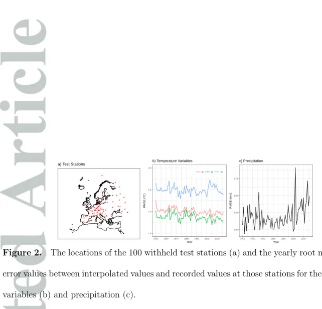
To assess the quality of the interpolation we have withheld 100 stations from the sample of stations available for gridding and we have then compared interpolated values against the recorded station values at those locations. Reference stations were selected initially by only retaining stations that were more than 90% complete over the 1950–2016 period for all four variables. A spatially even coverage of 100 stations was then selected using minimax sampling, which selects stations from the total number of available stations such that the maximum distance from the station to any of the other stations is minimized (Figure 2 a). Since the density of stations varies significantly over the domain (Figure 1) the use of a fixed sample of stations ensures that spatial bias in the testing is reduced, and also ensures that the reference station values take no part in either the background (monthly) field interpolation in the first stage of gridding, or the daily interpolations. A full leave-one-out cross validation was not possible given the number of stations involved and the time required to complete the interpolation.
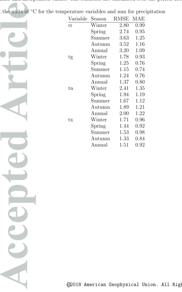
We have calculated error statistics (RMSE and mean absolute error [MAE]) between the interpolated values and reference stations over the period 1950–2016 (Table 1). In this analysis the interpolated values are the mean across the 100 realizations. For the temperature variables, RMSE values range from 1.15◦C to 2.41 ◦C. This error, however, is highly dependent upon the temperature variable or season considered. The highest errors are observed for daily minimum temperature and during the winter season. The
error values also vary seasonally in the case of daily precipitation totals, with RMSE values reaching a minimum of 2.74mm in the spring, and a maximum of 3.63mm in the summer. This is a reflection of the fact that winter precipitation will be more associated with fronts, and summer precipitation is more likely to be convective in nature.
The RMSE values also vary over time, although in the case of the temperature variables the stratification in RMSE values remains constant over the time period (Figure 2). In the case of precipitation the RMSE values exhibit relatively large year-to-year variation. The results for the tx and tg variables display a gradual reduction in RMSE values since 1950, although there is an indication of a step to slightly lower error values after 1990, especially in the results for tx. Interestingly, in the case of tn there is a step to higher RMSE values after the year 2001. An examination of the annual RMSE values on a station-by-station basis (not shown) reveals that these step changes only occur in some of the reference stations. Hence the temporal changes in RMSE are likely attributable to inhomogeneities in the reference stations rather than any particular change in the gridding. In light of these results, we reiterate the message of previous studies [Hofstra et al., 2009; Cornes
and Jones, 2013] that caution should be exercised when using the E-OBS dataset for the
examination of long-term trends across Europe as the station data have not undergone any homogeneity correction at present. Homogeneity testing is carried out on the stations
[The ECA&D Team, 2012] but this information is not taken into account when gridding
the data. Inhomogeneities in the gridded data are also likely as a result of the marked change in station numbers over time.
The discrepancy in error between tx and tn highlights a further feature of the E-OBS data that must be taken into consideration by data-users: since tx and tn are gridded
independently, there is no guarantee that individual daily tx values are greater than tn, despite the input station data being checked for this property. Similarly, there is no guarantee that interpolated tg values will be the mean of the tx and tn interpolations at the respective grid boxes, as may be expected given that this is one of the more widely used method of calculating tg in the station data. The number of occurrences of tx <tn varies over the time period, with up to 0.4% of grid-cells experiencing the problem in the last five years of the series, which seems to be a result of the use of more GTS-derived data during that period; prior to that the average of yearly counts of tx <tn occurrences is 0.06%.
3.2. Features of the ensemble
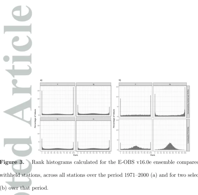
Rank histograms are a simple way of determining the reliability of an ensemble of real-izations relative to observations [Wilks, 2006]. They are calculated by ranking an ensemble from lowest to highest to form a series of n+ 1 bins, given n ensemble realizations; the highest and lowest bins are open-ended. The corresponding observed value is then allo-cated to the appropriate bin. This procedure is then repeated for different observation sites and/or different times to generate a large sample. Using the withheld station obser-vations from Section 3.1, rank histograms have been calculated for the E-OBS ensemble (Figure 3). In the case of precipitation, values are only used when non-zero precipitation occurred in the ensemble members and observations, after Bach et al.[2016].
The rank histograms calculated for all of the 100 station sites over the period 1971– 2000 (Figure 3 a) show a distinctive U-shape, with a much higher proportion of the observations falling in the first and last histogram bins compared to the central range of bins. This indicates that overall the ensemble is too optimistic in representing the
range of uncertainty, i.e. the ensemble samples are taken from a distribution with a lack of variability compared to the observations [Hamill, 2001]. However, the nature of the histograms varies considerably depending on the location of the observation station. For stations in the regions of higher station density, such as Germany or Sweden (see Figure 1), the rank histograms typically show a higher relative frequency in the central bins, which indicates an underestimation Typical examples are shown in Figure 3 b. This may result from the calculation of the ensemble using a single variogram for the entire region, which biases the spatial structure of the interpolated field, and hence the ensemble spread, to the spatial variation observed in the regions of higher station density. This feature may also result from a disparity in spatial variability captured in the GAM relative to the GRFs (see Section 2.3). For precipitation the picture is more complicated, and even in areas of high-station density an over-dispersion of observations occur in the outer bins of the histogram, as demonstrated for the station ‘Mainburg’ in Germany in Figure 3 b. However, for that station a relatively high dispersion is also apparent in the central bins. This pattern may indicate different degrees of spread-reliability under different precipitation regimes.
Discrimination and reliability diagrams are also useful ways of indicating the character-istics of an ensemble dataset and are used here to provide further information about the v16.0e precipitation ensemble. Discrimination diagrams show the distribution of the es-timated likelihood of events and non-events relative to the observed likelihood of events, while reliability diagrams display the observed conditional probability of an event ex-pressed as a function of the ensemble-estimated probability [Wilks, 2006]. Following the example of Clark et al.[2006] and Newman et al. [2015] these diagrams have been
calcu-lated using four thresholds (Figure 4). The discrimination diagrams (Figure 4 a) indicate that a good degree of separation exists in the discrimination of observed events greater than 0mm. It should be noted that the common masking of rainfall for all ensemble mem-bers on a given day results in a binary likelihood for rr>0mm in the ensemble probability; At the higher precipitation intensities a consistency is apparent in the probability of events compared to non-events, although there is a much better discrimination of event proba-bility when the estimated ensemble probaproba-bility is equal to one. This feature also results from the fixed precipitation masking, but the advantage comes at the expense of slightly reduced discrimination at the lower ensemble-estimated probabilities (c.f. the results in citet:Newman2015 who use a probabilistic method to estimate rainfall occurrence)
In accordance with the results from the discrimination diagrams, the reliability diagrams (Figure 4 b) indicate a slight dry bias in ensemble-estimated probabilities of precipitation occurrence below around 0.7 although these values are within the 5-95% consistency range. Above probabilities of around 0.6-0.7, a wet bias is apparent in the results, which is most apparent at the highest threshold level of rr>50.0mm.
In this section the ensemble values have been are compared against station values. In contrast, the gridded dataset aims to provide values that are representative of grid-box averages. Hence discrepancies would be expected in the comparisons, particularly for precipitation, and the results are consistent with interpolated values that smooth over station-scale values. The results for the temperature variables indicate, however, that the scale that is depicted in the interpolated values likely varies over the domain, with gridded values in areas with relatively high-station density resolving the temperature field at a smaller scale than in data-sparse regions. A similar conclusion was reached by Hofstra
et al.[2009] in their evaluation of the original version of E-OBS, but this discrepancy has likely become more pronounced as more stations have been added to certain areas (see Figure 1).
3.3. Comparison against the previous E-OBS version
In Figure 5 we compare the climatological annual averages (totals in the case of precip-itation) calculated over the period 1981–2010 from E-OBS v16.0 and v16.0e. In the case of temperature, the largest (negative) differences in the climatologies occur across North Africa and the Middle East. This is the region of lowest station density and hence these are the regions where the largest differences would be expected to occur. Across most other regions of Europe the differences are generally in the range ± 0.5 ◦C, and across many areas approach 0 ◦C. Larger differences tend to occur across mountainous regions, particularly the Alps, and this is likely a result of the significantly different methods used to incorporate the environmental lapse-rate in the two versions of E-OBS (as discussed in Section 2.2.1).
In the case of precipitation (Figure 5 c/d) the largest differences also tend to occur across North Africa and the Middle East, which likely result from a combination of the low density of stations, the associated high degree of uncertainty in the interpolation and the low average rainfall totals recorded in these regions. However, v16.0e is also wetter than v16.0 by around 5–10%, particularly across eastern regions of the gridded region. This is most probably a result of the method used to scale the daily precipitation anomalies by monthly totals in v16.0, compared to the incorporation of altitude in the spatial-trend model as a function of the monthly interpolation in v16.0e, and demonstrates
the sensitivity of precipitation grids to the choice of interpolation method [Sun et al., 2014;
Herold et al., 2016].
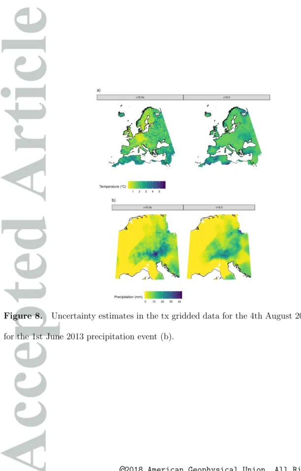
To further illustrate the differences between the two versions of E-OBS we have ex-amined the interpolations of maximum daily temperature for 4th August 2003 and daily precipitation for 1st June 2013. Both of these events represent very extreme events in the ECA&D record: the 2003 event was the climax of the exceptionally hot summer of 2003 [Garc´ıa-Herrera et al., 2010], and the precipitation event of 2013 led to significant flooding across the Upper Danube catchment [Bl¨oschl et al., 2013].
In the case of the 2003 event (Figure 6 a), the two versions of E-OBS are broadly consistent, with differences being generally less than 1 ◦ C. As with the climatological mean values, the largest differences tend to occur across North Africa, and likely reflects the poor data coverage in this region. Differences of more than -4 ◦C are also evident in certain other regions, notably southern Turkey and Western Russia, which also seem to be a result of the response of the different gridding methods to interpolating across data sparse regions.
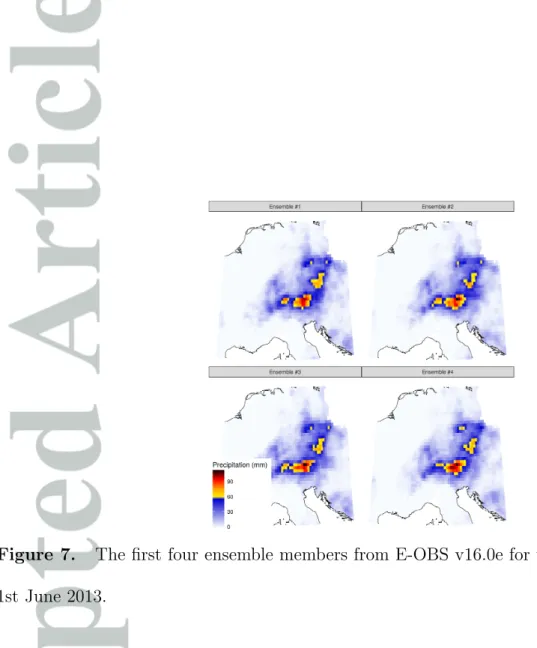
The spatial structure of the precipitation event of 2013 is broadly similar between the two versions of E-OBS, although differences of about 10 mm are apparent for certain grid-cells (Figure 6 c). The most intense precipitation is more concentrated in v16.0e, whereas the region experiencing>75 mm is larger in v16.0. As with the precipitation climatologies described above, this is likely a result of the method used in v16.0 of scaling the daily gridded field to the monthly precipitation totals. It should be noted, however, that there is considerable uncertainty in the precipitation totals for this event in E-OBS since the highest precipitation totals occurred in a region with relatively sparse data coverage as
well as being in a mountainous region. This uncertainty is demonstrated in Figure 7, which plots the first four ensemble members for this precipitation event.
In Figure 8 the uncertainty ranges for the two interpolations are plotted. In v16.0 this uncertainty is defined as 1.64 times the standard error (90% uncertainty, under the assumption of a normal distribution), whereas in v16.0e this is more strictly defined as the 90% range across the ensemble (see Section 2.3). Despite this difference in uncertainty-definition, in v16.0e these values are more closely related to station coverage than v16.0, which shows a much more smoothed field of uncertainty. This difference in spread between the two E-OBS versions is most pronounced for temperature, where the spread is much reduced at grid-cells close to stations, and in data rich regions, but is much larger in areas of low station density. In the rank histograms examined above, the ensemble was shown to be generally overly optimistic, but this appears to be a more realistic measure of uncertainty than was provided in E-OBS v16.0. The spread of uncertainty for precipitation is also much larger in data sparse regions, and is more closely linked to station density in v16.0e. However, the uncertainty for precipitation must also scale with interpolated totals
[Hutchinson, 1995b, 1998b]. Hence, in Figure 8 b the relationship to station coverage is
not as immediately apparent as in the temperature interpolation.
3.4. Comparison against NMSs gridded datasets
To further examine the differences between E-OBS v16.0e and v16.0, we have evaluated the datasets against several high-resolution regional datasets produced by various NMSs across Europe (Table 2). A variety of different interpolation procedures are used to construct these datasets but they are generally developed using many more station data than are available to E-OBS, although this disparity varies by dataset. In addition,
since these datasets are developed for discrete regions of Europe they suffer less from the constraints in E-OBS of the need to generalize the meteorological field across a large diverse domain, and with a greatly varying spatial density of station data. In the case of E-OBS, spatial variability is generalized using smoothing parameters fixed across the region, both in the GAM-derived spatial trend and in the simulated residuals (c.f. the piece-meal method used by Lussana et al. [2017]). For these reasons the NMSs datasets would be expected to provide a closer estimate of the true areal averages for their respective domains than E-OBS [Hofstra et al., 2008]. The NMSs datasets were regridded to the E-OBS 0.25
◦ x 0.25 ◦ regular grid using box-averaging. The NMSs data are generally produced on a
much higher resolution grid than E-OBS (Table 2), and hence these aggregated values are expected to be comparable to the box-average values of E-OBS. However, in the case of the PORT02 the resolution of 20km is comparable to E-OBS. In that case nearest-neighbour interpolation was used. No correction was applied for elevation differences between E-OBS and the NMSs data, since the main reason for conducting this comparison was to evaluate the two versions of E-OBS relative to the NMSs data.
In Figure 9 we have plotted the differences (E-OBS minus NMSs) in annual climatologies between the datasets for the variables tg and rr. These have been calculated over the period 1971–2010, which is common to all datasets. In general the differences in the two versions of E-OBS are comparable; the results for tx and tn are similar to those shown here for tg. In the case of tg, the smallest differences occur relative to the UKCP09 dataset, with the largest differences apparent when compared against the MeteoSwiss tg dataset, where both E-OBS datasets are warmer on average by more than 5◦ C across the high Alps. This is likely the result of there being more high-elevation stations available
for the MeteoSwiss interpolation. In the case of precipitation, both E-OBS versions show a dry bias relative to the NMSs datasets across most lower elevation regions, although a wet bias is apparent across most mountainous regions. There is an indication that this bias is substantially reduced in the new version of E-OBS when compared against the CARPATCLIM, EURO4M APGD PORT02 and SPAIN02 datasets.
To examine differences in daily extremes between the two versions of E-OBS, relative to the NMSs gridded datasets, we have sorted the absolute differences in daily values at each grid-box into deciles (Figure 10). The deciles are determined by the NMSs grid-box values. For precipitation the deciles are calculated for non-zero values, but a further category for zero precipitation values is included. Hofstra et al.[2008] performed a similar comparison in their examination of spatial interpolation methods, as a first stage in developing the original version of E-OBS.
The results indicate little difference in bias between the two versions of E-OBS, relative to the NMSs data. The differences between E-OBS v16.0 and v16.0e differ in only one case: for the variable tx, slightly higher biases in v16.0e are evident relative to the MeteoSwiss gridded data. In the case of precipitation, both of the datasets display the expected scaling of error with interpolated precipitation totals. In general, the results from both this analysis and the comparison of climatological biases indicate that the biases between the two versions of E-OBS are generally small compared to the actual differences between respective versions of E-OBS and the NMSs gridded data. This corresponds to the general finding ofHofstra et al.[2009], who evaluated gridding techniques for the ECA&D stations data relative to station data and NMSs gridded datasets in the development of the old version of E-OBS. Their study concluded that the interpolation technique had less of
an effect on the quality of the gridded data compared to the density and quality of input station data. While station density governs the biases observed here, the different interpolation methods and DEM data used in the NMSs gridded datasets probably also have an effect on the results.
4. Conclusions
In this paper we have described the construction of a new version of the E-OBS tem-perature (tn, tg and tx) and precipitation datasets. A 100-member ensemble of each daily field has been generated, which provides an improved estimation of uncertainty. In terms of both climatological averages and extreme values, the ensemble-mean grids in the new version of E-OBS are broadly comparable to the ‘best-guess’ grids in the earlier version and we stress that station coverage is the most important factor in determining the success of the gridded data. Nonetheless, users will notice differences between the two E-OBS versions, and this results from the different gridding methods used in the two versions of the dataset. Furthermore, while the ensemble mean can be taken as grid-box averages, the individual ensemble members display a spatial variation that is between a point and a box average value, although this discrepancy varies across the domain in relation to station density.
The uncertainty quantified by the ensemble dataset is more closely related to station density than uncertainty values in the original dataset, although the uncertainty in data-sparse regions, while much larger in these areas than in the original dataset, still appears to be an underestimate of the true uncertainty. The uncertainty quantified by the ensemble only relates to interpolation uncertainty, and improvements may be made in this estimate through the quantification of other sources of uncertainty such as instrumentation error
(e.g. Yang et al.[1999b]). More general improvements may be made to the E-OBS dataset through the use of additional explanatory variables such as slope/aspect, in the case of precipitation, or coastal proximity for temperature [Vose et al., 2014; Daly et al., 2008], or the embedding of non-gaussian distributions such as the Tweedie distributions [Hasan
and Dunn, 2011] in the spatial trend model. Changes to the relative scaling of altitude
to longitude/latitude coordinates could also be investigated in further updates to the dataset.
In this paper, the ensemble dataset has been produced to match the 0.25◦ grid resolution of earlier versions of E-OBS (regular grid spacing). A need exists to produce a version of E-OBS at a higher spatial resolution than the current ca. 25km resolution [Moreno
and Hasenauer, 2016]. A higher-resolution version of E-OBS is planned. In addition,
the original E-OBS gridding scheme has been used to construct a dataset of temperature and precipitation for southeast Asia [van den Besselaar et al., 2017], and the methods demonstrated in this paper will also be tested for that region, with a view to developing an ensemble dataset for the southeast Asia region. Furthermore, it remains the case that many of the input station series have not been homogenized and at present we caution against the use of E-OBS for evaluating trends. Efforts are currently underway to produce a version of E-OBS using homogenized station data.
5. Acknowledgements
We remain grateful to all data providers who supply station data to ECA&D. This work was funded by the European Union’s seventh Framework Programme (EU FP7) project “Uncertainties in Ensembles of Regional Re-Analyses (UERRA)” under grant agreement 607193, and the Copernicus Climate Change Service (C3S 311a lot4). The
CARPATCLIM gridded dataset forms part of the CARPATCLIM database (European Commission - JRC, 2013). The gridded temperature data for Switzerland were provided by the Federal Office of Meteorology and Climatology MeteoSwiss, and the SAFRAN dataset was provided by Meteo-France. We would like to thank the three reviewers for their insightful comments on the paper. The ECA&D/E-OBS data are available from https://www.ecad.eu and http://surfobs.climate.copernicus.eu.
References
Aalto, J., P. Pirinen, and K. Jylh¨a (2016), New gridded daily climatology of Finland: Permutation-based uncertainty estimates and temporal trends in climate, J. Geophys.
Res. Atmos., 121(8), 3807–3823, doi:10.1002/2015JD024651.
Bach, L., C. Schraff, J. D. Keller, and A. Hense (2016), Towards a probabilistic regional reanalysis system for Europe: Evaluation of precipitation from experiments,Tellus, Ser.
A Dyn. Meteorol. Oceanogr., 68(1), doi:10.3402/tellusa.v68.32209.
Beguer´ıa, S., S. M. Vicente-Serrano, M. Tom´as-Burguera, and M. Maneta (2016), Bias in the variance of gridded data sets leads to misleading conclusions about changes in climate variability, Int. J. Climatol., 36(9), 3413–3422, doi:10.1002/joc.4561.
Belo-Pereira, M., E. Dutra, and P. Viterbo (2011), Evaluation of global precipitation data sets over the Iberian Peninsula, J. Geophys. Res. Atmos., 116(20), 1–16, doi: 10.1029/2010JD015481.
Bl¨oschl, G., T. Nester, J. Komma, J. Parajka, and R. A. P. Perdig˜ao (2013), The June 2013 flood in the Upper Danube Basin, and comparisons with the 2002, 1954 and 1899 floods, Hydrol. Earth Syst. Sci., 17(12), 5197–5212, doi:10.5194/hess-17-5197-2013.
Br¨ocker, J., L. A. Smith, J. Br¨ocker, and L. A. Smith (2007), Increasing the Reliability of Reliability Diagrams, Weather Forecast., 22(3), 651–661, doi:10.1175/WAF993.1. Clark, M. P., A. G. Slater, M. P. Clark, and A. G. Slater (2006), Probabilistic
Quan-titative Precipitation Estimation in Complex Terrain, J. Hydrometeorol., 7(1), 3–22, doi:10.1175/JHM474.1.
Cornes, R. C., and P. D. Jones (2013), How well does the ERA-Interim reanalysis replicate trends in extremes of surface temperature across Europe?, J. Geophys. Res. Atmos.,
118(18), 10,262–10,276, doi:10.1002/jgrd.50799.
Dahlgren, P., T. Landelius, P. K˚allberg, and S. Gollvik (2016), A high-resolution regional reanalysis for Europe. Part 1: Three-dimensional reanalysis with the regional HIgh-Resolution Limited-Area Model (HIRLAM), Q. J. R. Meteorol. Soc., 142(698), 2119– 2131, doi:10.1002/qj.2807.
Daly, C., M. Halbleib, J. I. Smith, W. P. Gibson, M. K. Doggett, G. H. Taylor, J. Curtis, and P. P. Pasteris (2008), Physiographically sensitive mapping of climatological tem-perature and precipitation across the conterminous United States, Int. J. Climatol.,
28(15), 2031–2064, doi:10.1002/joc.1688.
Danielson, J. J., and D. Gesch (2011), Global multi-resolution terrain elevation data 2010 (GMTED2010),Tech. rep., U.S. Geological Survey Open-File Report 2011-1073. Frei, C. (2014), Interpolation of temperature in a mountainous region using
nonlin-ear profiles and non-Euclidean distances, Int. J. Climatol., 34(5), 1585–1605, doi: 10.1002/joc.3786.
Garc´ıa-Herrera, R., J. D´ıaz, R. M. R. M. Trigo, J. Luterbacher, and E. M. Fischer (2010), A Review of the European Summer Heat Wave of 2003, Crit. Rev. Environ. Sci.
Tech-nol.,40(4), 267–306, doi:10.1080/10643380802238137.
Hamill, T. M. (2001), Interpretation of Rank Histograms for Verifying En-semble Forecasts, Mon. Weather Rev., 129(3), 550–560, doi:10.1175/1520-0493(2001)129¡0550:IORHFV¿2.0.CO;2.
Hasan, M. M., and P. K. Dunn (2011), Two Tweedie distributions that are near-optimal for modelling monthly rainfall in Australia, Int. J. Climatol., 31(9), 1389–1397, doi: 10.1002/joc.2162.
Hastie, T., and R. Tibshirani (1990), Generalized additive models, 335 pp., Chapman & Hall/CRC.
Haylock, M. R., N. Hofstra, A. M. G. Klein Tank, E. J. Klok, P. D. Jones, and M. New (2008), A European daily high-resolution gridded data set of surface tem-perature and precipitation for 1950–2006, J. Geophys. Res., 113(D20), D20,119, doi: 10.1029/2008JD010201.
Herold, N., L. V. Alexander, M. G. Donat, S. Contractor, and A. Becker (2016), How much does it rain over land?,Geophys. Res. Lett.,43(1), 341–348, doi:10.1002/2015GL066615. Herrera, S., J. Fern´andez, and J. M. Guti´errez (2016), Update of the Spain02 gridded observational dataset for EURO-CORDEX evaluation: assessing the effect of the inter-polation methodology, Int. J. Climatol., 36(2), 900–908, doi:10.1002/joc.4391.
Hewitson, B. C., and R. G. Crane (2005), Gridded area-averaged daily precipitation via conditional interpolation, J. Clim., 18(1), 41–57, doi:10.1175/JCLI3246.1.
Hofstra, N., M. Haylock, M. New, P. Jones, and C. Frei (2008), Comparison of six methods for the interpolation of daily, European climate data, J. Geophys. Res., 113(D21), D21,110, doi:10.1029/2008JD010100.
Hofstra, N., M. Haylock, M. New, and P. D. Jones (2009), Testing E-OBS European high-resolution gridded data set of daily precipitation and surface temperature, J. Geophys. Res., 114(D21), D21,101, doi:10.1029/2009JD011799.
Hutchinson, M. F. (1995a), Stochastic space-time weather models from ground-based data, Agric. For. Meteorol.,73(3-4), 237–264, doi:10.1016/0168-1923(94)05077-j. Hutchinson, M. F. (1995b), Interpolating mean rainfall using thin plate smoothing splines,
Int. J. Geogr. Inf. Syst., 9(4), 385–403, doi:10.1080/02693799508902045.
Hutchinson, M. F. (1998a), Interpolation of Rainfall Data with Thin Plate Smoothing Splines - Part I: Two Dimensional Smoothing of Data with Short Range Correlation,J.
Geogr. Inf. Decis. Anal.,2, 168–185.
Hutchinson, M. F. (1998b), Interpolation of rainfall data with thin plate smoothing splines - Part II: Analyis of topographic dependence,J. Geogr. Inf. Decis. Anal.,2(2), 152–167. Hutchinson, M. F., and X. Tingbao (2013), Anusplin Version 4.4 User Guide,Tech. rep., The Australian National University Fenner School of Environment and Society, Can-berra.
Hutchinson, M. F., D. W. McKenney, K. Lawrence, J. H. Pedlar, R. F. Hopkinson, E. Milewska, and P. Papadopol (2009), Development and testing of Canada-wide inter-polated spatial models of daily minimum-maximum temperature and precipitation for 1961-2003,J. Appl. Meteorol. Climatol.,48(4), 725–741, doi:10.1175/2008JAMC1979.1. Isotta, F. A., C. Frei, V. Weilguni, M. Perˇcec Tadi´c, P. Lass`egues, B. Rudolf, V. Pa-van, C. Cacciamani, G. Antolini, S. M. Ratto, M. Munari, S. Micheletti, V. Bonati, C. Lussana, C. Ronchi, E. Panettieri, G. Marigo, and G. Vertaˇcnik (2014), The cli-mate of daily precipitation in the Alps: development and analysis of a high-resolution
grid dataset from pan-Alpine rain-gauge data,Int. J. Climatol., 34(5), 1657–1675, doi: 10.1002/joc.3794.
Isotta, F. A., R. Vogel, and C. Frei (2015), Evaluation of European regional reanalyses and downscalings for precipitation in the Alpine region, Meteorol. Zeitschrift, 24(1), 15–37, doi:10.1127/metz/2014/0584.
Jermey, P. M., and R. J. Renshaw (2016), Precipitation representation over a two-year period in regional reanalysis, Q. J. R. Meteorol. Soc., 142(696), 1300–1310, doi: 10.1002/qj.2733.
Kim, Y.-J., and C. Gu (2004), Smoothing spline Gaussian regression: more scalable computation via efficient approximation,J. R. Stat. Soc. Ser. B (Statistical Methodol.,
66(2), 337–356, doi:10.1046/j.1369-7412.2003.05316.x.
Klein Tank, A. M. G., J. B. Wijngaard, G. P. K¨onnen, R. B¨ohm, G. Demar´ee, A. Gocheva, M. Mileta, S. Pashiardis, L. Hejkrlik, C. Kern-Hansen, R. Heino, P. Bessemoulin, G. M¨uller-Westermeier, M. Tzanakou, S. Szalai, T. P´alsd´ottir, D. Fitzgerald, S. Rubin, M. Capaldo, M. Maugeri, A. Leitass, A. Bukantis, R. Aberfeld, A. F. V. van Engelen, E. Forland, M. Mietus, F. Coelho, C. Mares, V. Razuvaev, E. Nieplova, T. Cegnar, J. Antonio L´opez, B. Dahlstr¨om, A. Moberg, W. Kirchhofer, A. Ceylan, O. Pachal-iuk, L. V. Alexander, and P. Petrovic (2002), Daily dataset of 20th-century surface air temperature and precipitation series for the European Climate Assessment, Int. J.
Climatol., 22(12), 1441–1453.
Klok, E. J., and A. M. G. Klein Tank (2009), Updated and extended European dataset of daily climate observations, Int. J. Climatol., 29(8), 1182–1191.
Lavaysse, C., C. Camalleri, A. Dosio, G. van der Schrier, A. Toreti, and J. Vogt (2017), Towards a monitoring system of temperature extremes in Europe, Nat. Hazards Earth
Syst. Sci. Discuss., pp. 1–29, doi:10.5194/nhess-2017-181.
Legates, D. R., and C. J. Willmott (1990), Mean seasonal and spatial variabil-ity in gauge-corrected, global precipitation, Int. J. Climatol., 10(2), 111–127, doi: 10.1002/joc.3370100202.
Lenderink, G. (2010), Exploring metrics of extreme daily precipitation in a large en-semble of regional climate model simulations, Clim. Res., 44(2-3), 151–166, doi: 10.3354/cr00946.
Lussana, C., O. Tveito, and F. Uboldi (2017), Three-dimensional spatial interpolation of two-meter temperature over Norway, Q. J. R. Meteorol. Soc., doi:10.1002/qj.3208. Masson, D., and C. Frei (2014), Spatial analysis of precipitation in a high-mountain
region: exploring methods with multi-scale topographic predictors and circulation types,
Hydrol. Earth Syst. Sci., 18(11), 4543–4563, doi:10.5194/hess-18-4543-2014.
Min, E., W. Hazeleger, G. J. van Oldenborgh, and A. Sterl (2013), Evaluation of trends in high temperature extremes in north-western Europe in regional climate models,
En-viron. Res. Lett., 8(1), 14,011.
Mohr, C. (2009), Comparison of versions 1.1 and 1.0 of gridded temperature and precipi-tation data for Norway, Tech. rep., (Met. No. Note 19/2009) Norwegian Meteorological Institute, Oslo.
Moreno, A., and H. Hasenauer (2016), Spatial downscaling of European climate data,Int.
Morice, C. P., J. J. Kennedy, N. A. Rayner, and P. D. Jones (2012), Quantifying uncer-tainties in global and regional temperature change using an ensemble of observational estimates: The HadCRUT4 data set, J. Geophys. Res. Atmos., 117(8), D08,101, doi: 10.1029/2011jd017187.
Neff, E. L. (1977), How much rain does a rain gage gage?, J. Hydrol., 35(3-4), 213–220, doi:10.1016/0022-1694(77)90001-4.
Newman, A. J., M. P. Clark, J. Craig, B. Nijssen, A. Wood, E. Gutmann, N. Mizukami, L. Brekke, and J. R. Arnold (2015), Gridded Ensemble Precipitation and Temperature Estimates for the Contiguous United States, J. Hydrometeorol.,16(6), 2481–2500, doi: 10.1175/JHM-D-15-0026.1.
Nikulin, G., E. Kjellstrom, U. L. F. Hansson, G. Strandberg, and A. Ullerstig (2011), Evaluation and future projections of temperature, precipitation and wind extremes over Europe in an ensemble of regional climate simulations, Tellus A, 63(1), 41–55.
Perry, M. C., D. M. Hollis, and M. Elms (2009), The generation of daily gridded datasets of temperature and rainfall for the UK.,Tech. rep., Met Office, National Climate Infor-mation Centre.
Schabenberger, O., and C. A. Gotway (2005),Statistical methods for spatial data analysis, 488 pp., Chapman & Hall/CRC.
Spinoni, J., S. Szalai, T. Szentimrey, M. Lakatos, Z. Bihari, A. Nagy, ´A. N´emeth, T. Kov´acs, D. Mihic, M. Dacic, P. Petrovic, A. Krˇziˇc, J. Hiebl, I. Auer, J. Milkovic, P. ˇStep´anek, P. Zahradn´ıcek, P. Kilar, D. Limanowka, R. Pyrc, S. Cheval, M.-V. Bir-san, A. Dumitrescu, G. Deak, M. Matei, I. Antolovic, P. Nejedl´ık, P. ˇStastn´y, P. Ka-jaba, O. Bochn´ıcek, D. Galo, K. Mikulov´a, Y. Nabyvanets, O. Skrynyk, S. Krakovska,
N. Gnatiuk, R. Tolasz, T. Antofie, and J. Vogt (2015), Climate of the Carpathian Re-gion in the period 1961-2010: climatologies and trends of 10 variables,Int. J. Climatol.,
35(7), 1322–1341, doi:10.1002/joc.4059.
Sun, Q., C. Miao, Q. Duan, D. Kong, A. Ye, Z. Di, and W. Gong (2014), Would the real’ observed dataset stand up? A critical examination of eight observed grid-ded climate datasets for China, Environ. Res. Lett., 9(1), 015,001, doi:10.1088/1748-9326/9/1/015001.
The ECA&D Team (2012), European Climate Assessment & Dataset Algorithm Theoreti-cal Basis Document (ATBD), version 10.5,Tech. rep., Royal Netherlands Meteorological Institute KNMI, De Bilt, NL.
van den Besselaar, E. J. M., M. R. Haylock, G. van der Schrier, and A. M. G. Klein Tank (2011), A European daily high-resolution observational gridded data set of sea level pressure,J. Geophys. Res. Atmos., 116(11), 1–11, doi:10.1029/2010JD015468.
van den Besselaar, E. J. M., A. M. G. Klein Tank, G. van der Schrier, and P. D. Jones (2012), Synoptic messages to extend climate data records, J. Geophys. Res. Atmos.,
117(D7), doi:10.1029/2011JD016687.
van den Besselaar, E. J. M., G. van der Schrier, R. C. Cornes, A. S. Iqbal, and A. M. G. Klein Tank (2017), SA-OBS: A Daily Gridded Surface Temperature and Precipita-tion Dataset for Southeast Asia, J. Clim., 30(14), 5151–5165, doi:10.1175/JCLI-D-16-0575.1.
van der Schrier, G., E. J. M. van den Besselaar, A. M. G. Klein Tank, and G. Verver (2013), Monitoring European average temperature based on the E-OBS gridded data
van Oldenborgh, G. J., S. Philip, E. Aalbers, R. Vautard, F. Otto, K. Haustein, F. Habets, R. Singh, and H. Cullen (2016), Rapid attribution of the May/June 2016 flood-inducing precipitation in France and Germany to climate change, Hydrol. Earth Syst. Sci.
Dis-cuss., 2016, 1–23, doi:10.5194/hess-2016-308.
Vidal, J.-P., E. Martin, L. Franchist´eguy, M. Baillon, and J.-M. Soubeyroux (2010), A 50-year high-resolution atmospheric reanalysis over France with the Safran system,Int.
J. Climatol., 30(11), 1627–1644, doi:10.1002/joc.2003.
Vose, R. S., S. Applequist, M. Squires, I. Durre, M. J. Menne, C. N. Williams, C. Fenimore, K. Gleason, and D. Arndt (2014), Improved Historical Temperature and Precipitation Time Series for U.S. Climate Divisions,J. Appl. Meteorol. Climatol.,53(5), 1232–1251, doi:10.1175/JAMC-D-13-0248.1.
Wilks, D. S. (2006), Statistical Methods in the Atmospheric Sciences, 2nd editio ed., Academic Press.
Wood, S. (2014), mgcv: Mixed GAM Computation Vehicle with GCV/AIC/REML smoothness estimation.
Wood, S. N. (2003), Thin plate regression splines, J. R. Stat. Soc. Ser. B (Statistical
Methodol., 65(1), 95–114, doi:10.1111/1467-9868.00374.
Wood, S. N. (2006),Generalized Additive Models: An Introduction with R, Chapman and Hall/CRC.
Yamamoto, J. K. (2000), An alternative measure of the reliability of ordinary kriging estimates, Math. Geol., 32(4), 489–509, doi:10.1023/A:1007577916868.
Yang, D., E. Elomaa, A. Tuominen, A. Aaltonen, B. Goodison, T. Gunther, V. Golubev, B. Sevruk, H. Madsen, and J. Milkovic (1999a), Wind-induced Precipitation Undercatch
of the Hellmann Gauges, Hydrol. Res., 30(1), 57–80, doi:10.2166/nh.1999.0004.
Yang, D., E. Elomaa, A. Tuominen, A. Aaltonen, B. Goodison, T. Gunther, V. Golubev, B. Sevruk, H. Madsen, and J. Milkovic (1999b), Wind-induced Precipitation Undercatch of the Hellmann Gauges, Hydrol. Res., 30(1), 57 LP – 80.
Table 1. Seasonal and annual RMSE and MAE statistics between the 100 reference station values and interpolated values. The statistics are calculated over the period 1950–2016 and are in the units of ◦C for the temperature variables and mm for precipitation
Variable Season RMSE MAE
rr Winter 2.80 0.99 Spring 2.74 0.95 Summer 3.63 1.25 Autumn 3.52 1.16 Annual 3.20 1.09 tg Winter 1.78 0.93 Spring 1.25 0.76 Summer 1.15 0.74 Autumn 1.24 0.76 Annual 1.37 0.80 tn Winter 2.41 1.35 Spring 1.94 1.19 Summer 1.67 1.12 Autumn 1.89 1.21 Annual 2.00 1.22 tx Winter 1.71 0.96 Spring 1.44 0.92 Summer 1.53 0.98 Autumn 1.33 0.84 Annual 1.51 0.92
Table 2. Details about the NMSs gridded datasets used for comparison against E-OBS. The resolution refers to the native resolution of the dataset.
Dataset Region Version Resolution Reference
tn tg tx rr
CARPATCLIM Carpathian basin x x x x - 10km Spinoni et al.[2015]
EURO4M APGD Greater Alpine x 1.0 5km Isotta et al.[2014]
MeteoSwiss Switzerland x x x 1.2 1km Frei [2014]
MET NO Norway x x 1.1 1km Mohr [2009]
PORT02 Portugal x - ∼20km Belo-Pereira et al.[2011]
SAFRAN France x x - 8km Vidal et al. [2010]
SPAIN02 Spain x x x AA-3D v4 ∼10km Herrera et al.[2016]