University of Central Florida University of Central Florida
STARS
STARS
Electronic Theses and Dissertations, 2004-20192009
Scalable And Efficient Outlier Detection In Large Distributed Data
Scalable And Efficient Outlier Detection In Large Distributed Data
Sets With Mixed-type Attributes
Sets With Mixed-type Attributes
Anna KoufakouUniversity of Central Florida
Part of the Computer Engineering Commons
Find similar works at: https://stars.library.ucf.edu/etd University of Central Florida Libraries http://library.ucf.edu
This Doctoral Dissertation (Open Access) is brought to you for free and open access by STARS. It has been accepted for inclusion in Electronic Theses and Dissertations, 2004-2019 by an authorized administrator of STARS. For more information, please contact [email protected].
STARS Citation STARS Citation
Koufakou, Anna, "Scalable And Efficient Outlier Detection In Large Distributed Data Sets With Mixed-type Attributes" (2009). Electronic Theses and Dissertations, 2004-2019. 3986.
Scalable and Efficient Outlier Detection in Large
Distributed Data Sets with Mixed-Type Attributes
by
Anna Koufakou
B.S. Athens University of Economics and Business, 1997 M.S. University of Central Florida, 2000
A dissertation submitted in partial fulfillment of the requirements for the degree of Doctor of Philosophy
in the School of Electrical Engineering and Computer Science in the College of Engineering
at the University of Central Florida Orlando, Florida
Summer Term 2009
Major Professor: Michael Georgiopoulos
c
Abstract
An important problem that appears often when analyzing data involves identifying irregular or abnormal data points called outliers. This problem broadly arises under two scenarios: when outliers are to be removed from the data before analysis, and when useful information or knowledge can be extracted by the outliers themselves. Outlier Detection in the context of the second scenario is a research field that has attracted significant attention in a broad range of useful applications. For example, in credit card transaction data, outliers might indicate potential fraud; in network traffic data, outliers might represent potential intrusion attempts.
The basis of deciding if a data point is an outlier is often some measure or notion of dissimilarity between the data point under consideration and the rest. Traditional outlier detection methods assume numerical or ordinal data, and compute pair-wise distances between data points. However, the notion of distance or similarity for categorical data is more difficult to define. Moreover, the size of currently available data sets dictates the need for fast and scalable outlier detection methods, thus precluding distance computa-tions. Additionally, these methods must be applicable to data which might be distributed among different locations.
In this work, we propose novel strategies to efficiently deal with large distributed data containing mixed-type attributes. Specifically, we first propose a fast and
scal-able algorithm for categorical data (AVF), and its parallel version based on MapReduce (MR-AVF). We extend AVF and introduce a fast outlier detection algorithm for large distributed data with mixed-type attributes (ODMAD). Finally, we modify ODMAD in order to deal with very high-dimensional categorical data. Experiments with large real-world and synthetic data show that the proposed methods exhibit large performance gains and high scalability compared to the state-of-the-art, while achieving similar accuracy detection rates.
Acknowledgments
I would like to take the opportunity to acknowledge a number of individuals for their support during my doctoral work. First, I would like to express many thanks to my adviser, Dr. Georgiopoulos, for providing me with his guidance and support these past many years. I would also like to thank my committee members, Dr. Eaglin, Dr. Kasparis, Dr. Reynolds, and Dr. Turgut for their time and their feedback, as well as Dr. Tace Crouse for her encouragement and advice.
I am very grateful to the many friends and colleagues who have shared my graduate experience at UCF with me, especially Pradeep, Jimmy, Moataz, Barry, Sasha, Maria. Also, many thanks to everyone at the UCF Women in EECS group, who have truly encouraged and inspired me this last year. I would also like to acknowledge all my friends outside UCF, especially Ioanna, Andreas, George, Parisa, and Mike. Finally, I would like to thank my parents for their endless encouragement and belief in me, my aunt Lela for her unconditional love, my sister and her family for their support, my aunt Korina for inspiring me, and my extended family for their encouragement.
This dissertation acknowledges the support by the National Science Foundation grants: 0341601, 0647018, 0717674, 0717680, 0647120, 0525429, 0806931, 0837332.
TABLE OF CONTENTS
LIST OF FIGURES . . . xi
LIST OF TABLES . . . xiv
CHAPTER 1: INTRODUCTION . . . 1
CHAPTER 2: PREVIOUS WORK . . . 9
2.1 Outlier Detection . . . 9
2.1.1 Statistical/Model-based Approaches . . . 9
2.1.2 Distance-based and Clustering Approaches . . . 10
2.1.3 Density-based Approaches . . . 12
2.1.4 Other Approaches. . . 13
2.1.5 Approaches for Data Sets with Categorical or Mixed-Type At-tributes . . . 14
2.2 Frequent Itemset Mining (FIM) . . . 15
2.2.1 Association Rule Mining and Traditional FIM . . . 15
2.2.2 Condensed Representations of FIs (CFIs) . . . 18
CHAPTER 3: OUTLIER DETECTION FOR CATEGORICAL DATA:
ATTRIBUTE VALUE FREQUENCY (AVF) . . . 21
3.1 Introduction . . . 21
3.2 Greedy Algorithm. . . 22
3.3 FindFPOF . . . 24
3.4 Otey’s Method for Categorical Data . . . 25
3.5 Attribute Value Frequency (AVF) . . . 27
3.6 Experiments . . . 29
3.6.1 Experimental Setup. . . 29
3.6.2 Results and Discussion . . . 30
3.7 Summary . . . 35
CHAPTER 4: PARALLEL OUTLIER DETECTION FOR CATEGORI-CAL DATASETS USING MAPREDUCE: MR-AVF . . . 37
4.1 Introduction . . . 37 4.2 Background on MapReduce . . . 38 4.3 MR-AVF. . . 42 4.4 MR-AVF Experiments . . . 44 4.4.1 Experimental Setup. . . 44 4.4.2 Results. . . 45 4.5 Summary . . . 46
CHAPTER 5: OUTLIER DETECTION FOR LARGE DISTRIBUTED
MIXED-ATTRIBUTE DATA: ODMAD . . . 48
5.1 Introduction . . . 48
5.2 Related Work . . . 50
5.3 Algorithms. . . 52
5.3.1 Centralized Algorithm . . . 53
5.3.2 Distributed Algorithm . . . 71
5.4 Experiments and Results . . . 74
5.4.1 Experimental Setup. . . 74 5.4.2 Results. . . 76 5.4.3 Distributed Experiments . . . 80 5.4.4 Additional Experiments . . . 81 5.4.5 Discussion . . . 87 5.5 Summary . . . 89
CHAPTER 6: OUTLIER DETECTION FOR LARGE CATEGORICAL DATA SETS USING NON-DERIVABLE (NDI) AND NON-ALMOST DERIVABLE (NADI) ITEMSETS . . . 91
6.1 Introduction . . . 91
6.2 Algorithms. . . 94
6.2.2 Outlier Detection based on NDIs: FNDI-OD . . . 101
6.2.3 Outlier Detection based on Approximation of NDIs . . . 111
6.3 Experiments . . . 113 6.3.1 Experimental Setup. . . 113 6.3.2 Results. . . 115 6.3.3 Discussion . . . 121 6.4 Summary . . . 127 CHAPTER 7: CONCLUSION . . . 129 7.1 Conclusions . . . 129
7.2 Discussion and Future Work . . . 131
APPENDIX A: NOTATION . . . 134
APPENDIX B: DATASETS. . . 136
APPENDIX C: COMPUTATIONAL SAVINGS DUE TO ODMAD CAT-EGORICAL SCORE . . . 142
LIST OF FIGURES
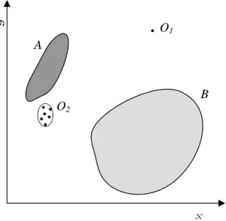
1 Two-Dimensional example of normal points (shaded regionsAandB) and outliers (O1,2). . . 2
2 Example of Frequent Sets, Infrequent Sets, and Sets on Negative Border. 16
3 Greedy Algorithm Pseudocode . . . 23 4 FindFPOF Pseudocode . . . 25 5 Otey’s Pseudocode (Categorical Data) . . . 26 6 Example of normal and outlier points from UCI Breast Cancer Dataset.
Outlier points are denoted by asterisk. . . 28 7 AVF Pseudocode . . . 29 8 AVF, Greedy, FPOF, and Otey’s runtime performance for simulated data
asn,k, and m increase (milliseconds). . . 33
9 The flow of data in a MapReduce/GFS architecture for file storage and MapReduce operations (dashed lines indicate control messages, and solid lines indicate data transfer). . . 41 10 A pictorial illustration of the WordCount example. . . 42 11 MR-AVF Pseudocode . . . 43
12 Speedup of Parallel AVF algorithm (MR-AVF) as the number of servers in the cluster increases from 1 node to 16 nodes. . . 46
13 Masking Effect: Outlier pointO2 is more irregular than the normal points
and outlier pointO1, thereforeO2 will likely mask O1.. . . 54
14 Scenarios for outlier points and normal points in the continuous space (dots denote normal points, diamonds denote outliers). Outlier points O2 have
a high categorical score, while outlier O1 has a low categorical score. In
the continuous space, outliers O2 are (a) highly irregular, (b) moderately
irregular, or (c) normal, with respect to the rest of the points (normal points and outlierO1). . . 66
15 First Phase of ODMAD Pseudocode . . . 68 16 Second Phase of ODMAD Pseudocode . . . 69 17 Categorical value b co-occurs in our dataset with highly infrequent
cate-gorical (a) value a only; (b) values a and c. . . 74 18 Speedup of ODMAD as the number of nodes increases from 2 to 16 for
the Entire KDDCup 1999 Dataset and Artificial Dataset (1 million normal points and 10 thousand outliers) . . . 81 19 Effect to detection rates for ODMAD on the KDDCup 1999 10% dataset
varying the lower thresholdlow sup (upper sup=σ = 10%; ∆scorec= 9, ∆scoreq = 1.6). . . 83
20 Effect to detection rates for ODMAD on the KDDCup 1999 10% dataset varying the upper thresholdupper sup(low sup = 2%;σ = 10%; ∆scorec=
9, ∆scoreq = 1.6). . . 84
21 Execution Time in seconds as the number of categorical and continuous attributes increases (Entire KDDCup 1999 set). . . 86
22 FI-OD Pseudocode . . . 98
23 NBFI-OD Pseudocode . . . 99
24 FNDI-OD Pseudocode . . . 109
25 NBNDI-OD Pseudocode . . . 111
26 Runtime performance for FNDI-OD vs. FI-OD for the Mushroom and KDD1999 sets as σ decreases (MAXLEN = 4). . . 119
27 Effect ofMAXLEN on the Correct Detection rates for NBNDI-OD versus NBFI-OD for the Mushroom set and two σ values.. . . 122
28 Correct Detection for FNADI-OD versus FNDI-OD for the Mushroom set and various δ values. . . 125
LIST OF TABLES
1 Algorithms presented in this dissertation and their characteristics w.r.t. attribute type, time complexity for categorical (mc) and continuous (mq) attributes, location of the dataset, and challenges they address. . . 8
2 AVF, Greedy, FPOF, and Otey’s Accuracy Results on Real Datasets . . 32 3 Runtime of AVF, Greedy, FPOF, and Otey’s Approaches in seconds for
the simulated data with varying number of data points, n. . . 34
4 Detection Rate of ODMAD vs. Otey’s on KDDCup 1999 (10%, Entire Training and Test Sets.) . . . 79 5 Execution Time (seconds) for ODMAD versus Otey’s on the KDDCup
1999 Datasets.. . . 80 6 ODMAD Detection Rate using only categorical attributes: all infrequent
subsets versus only pruned candidates, using the KDDCup 1999 10% Train Dataset. . . 88
7 Dataset Details: Number of rows, columns, single distinct items, percent-age of outliers in the dataset. . . 114
8 Comparison of Correct Detection (False Alarm) rates of FNDI-OD, FI-OD, NBNDI-FI-OD, and NBFI-OD for BC as k varies (σ = 10%; actual outliers: 39).. . . 116 9 Comparison of Correct Detection (False Alarm) rates of FNDI-OD, FI-OD,
NBNDI-OD, and NBFI-OD for (a)Mushroom and (b)KDD1999 Datasets. 116 10 Generated sets and Runtime performance for NDI- versus FI-based
meth-ods on the Mushroom and the KDD1999 set. Time is shown in seconds as Time for Phase 1 (Set Mining)/Time for Phase 2 (Outlier Scoring). . . 118 11 Comparison of Correct Detection (False Alarm) rates, Generated Sets, and
Runtime Performance in seconds for FI-OD, FNDI-OD, and FNADI-OD for (a)Mushroom and (b)KDD1999 Data Sets. . . 123 12 Frequency of distinct values (items) in Mushroom and KDD1999 Data
Sets. . . 127
13 Notation used in this dissertation. . . 135
CHAPTER 1
INTRODUCTION
The need for data mining, i.e. extracting knowledge from the data in the form of useful and interesting models and trends, is of greater importance today than ever before, due to the massive amount of data existing in databases all over the world. For example, it was projected that, by the end of 2007, the Sloan Digital Sky Survey1 will have produced
over 40 terabytes of image data, and over 3 terabytes of processed data.
Mining for outliers in data is an important data mining research field with many applications such as network intrusion detection [DEK02]. Outlier detection approaches focus on discovering patterns that occur infrequently in the data, as opposed to many traditional data mining techniques, such as association rule mining or frequent itemset mining, that attempt to find patterns that occur frequently in the data. One of the most widely accepted definitions of an outlier pattern is provided by Hawkins [Haw80]:
“An outlier is an observation that deviates so much from other observations as to arouse suspicion that it was generated by a different mechanism”.
Outliers are frequently treated as noise that needs to be removed from a dataset in order for a specific model or algorithm to succeed (e.g. points not belonging in clusters in a clustering algorithm). Alternatively, outlier detection techniques can lead to the
x y O 1 O2 A B
Figure 1: Two-Dimensional example of normal points (shaded regions A and
B) and outliers (O1,2).
discovery of important information in the data (“one person’s noise is another persons signal” [KN98]). Finally, outlier detection strategies can also be used for data cleaning as a step before any traditional mining algorithm is applied to the data.
It should be noted that this dissertation deals with unsupervised outlier detection, i.e. our methods do not assume labeled training data. Also, our techniques make the implicit assumption that the percentage of normal points is far larger compared to the percentage of outliers in the data set.
A pictorial two-dimensional example is shown in Figure 1. This Figure contains two groups or clusters of normal data points, denoted by shaded regions A and B, a single outlier point, O1, and a group of outlier points,O2.
Examples of applications where the discovery of outliers is useful include: detecting irregular credit card transactions which may indicate potential credit card fraud [BH02]; identifying patients who exhibit abnormal symptoms due to their suffering from a specific
disease or ailment [PJ01]; detecting irregularities and potential fraud in accounting data [BKA06], among others.
Many existing approaches are based on assumptions of a normal model/distribution or on calculating distances between each and every data point. For example, if we assume that outliers are those points that are most distant from the rest of the points, in Figure 1, outlierO1 is easily flagged as an outlier as being far from the rest of the points. However,
outlier points in region O2 are very close to normal points in region A and thus might
be more difficult to be detected as outliers. Therefore, more sophisticated algorithms are needed that can address these and other issues, described below.
In general, the performance and even the applicability of the majority of existing methods are limited by the characteristics of datasets currently available. Specifically, important challenges faced by outlier detection methods and addressed in this dissertation include the following:
(a) datasets might have large numbers of data points and dimensions,
(b) datasets might contain categorical attributes or a mixture of categorical and contin-uous attributes,
(c) challenges caused by the high dimensionality of the data, e.g. datasets might be sparse in the continuous space, or dense in the categorical space, and
(d) the points in the dataset might be distributed among different locations.
Large Number of Data Points and Dimensions: The first challenge mentioned
earlier is related to the large size of today’s data. With the explosion of technology, the size of data for a particular application has grown and will continue to grow; terabyte-scale data is now common, e.g., Wal-Mart had 460 terabytes of data in 2004 [Hay04]. Hence, successful outlier detection strategies must scale well as the number of data points and dataset dimensionality grow. The size of the datasets today also leads to the need for large, parallel machines and associated parallelizable outlier detection algorithms, which must also be easily balanced over a number of cluster nodes.
Types of Attributes: A second issue is that the majority of existing research in
outlier detection has focused on data sets with a specific attribute type, i.e. only numer-ical attributes or ordinal attributes that can be directly mapped into numernumer-ical values, while there is some research using only categorical attributes. Quite often, when we have data containing categorical attributes, for example, it is assumed that the categorical at-tributes could be easily mapped into numerical values. However, there are cases, where mapping categorical attributes to numerical attributes is not a straightforward process, and the results greatly depend on the mapping that is used, e.g., the mapping of a mari-tal status attribute value (married or single) or a person’s profession (engineer, financial analyst, etc.) to a numerical value.
In the case of continuous attributes, algorithms designed for categorical data often use discretization techniques to map intervals of continuous space into discrete values. Among unsupervised methods, i.e. those that do not use class information, popular algorithms include equal-width or equal-frequency binning. These methods might not produce good
results when the distributions of the continuous attribute values are not uniform, and the resulting discretized ranges are significantly affected by outliers [Cat91]. In our case, for example, values that are associated with normal points and values associated with outliers might be combined in the same bin, which makes the outlier detection task more difficult.
High Dimensionality of the Data: A third issue is due to the large number of
dimensions in the dataset. In the continuous space, due to the large dimensionality, the dataset becomes sparse. In this type of setting, traditional concepts such as Euclidean distance between points, and nearest neighbor, become irrelevant [ESK03]. Employing dissimilarity measures that can handle sparse data becomes imperative. In addition, inspecting several, smaller views of the large, high-dimensional data can help uncover outliers, which would otherwise be masked by other outlier points if one were to look at the entire dataset at once.
In the categorical space, certain datasets may contain many strong correlations, and are typically characterized by categorical values with high frequency and many frequent patterns [ZH05]. As a result, there might be a large number of combinations of these values to generate and store. In general, outlier detection in large high-dimensional data with many categorical values will also face issues if they are based on Frequent Itemsets [AS94].
Distributed Datasets: A fourth issue is that data may be distributed among differ-ent sites belonging to the same or differdiffer-ent organizations. Moreover, each of these sites might contain large amounts of data. This is an issue that has to be taken into account
for any data mining algorithm developed on such a platform, as for example moving or copying large amounts of data from site to site or storing all the data in one site in order to mine the dataset as a whole would be prohibitive. Besides the cost and performance issues, there are also very important issues related to data ownership and control which prohibit organizations from sharing data. Therefore, in order to deal with the distributed nature of the data, the outlier detection algorithms must minimize communication over-head and synchronization overover-head between the different sites in which the data reside, as well as the scans over the data.
The aim of this dissertation is to propose novel outlier detection techniques that are scalable and exhibit acceptable runtime performance given data sets that might be large, high-dimensional, geographically distributed, and contain categorical or a mixture of categorical and continuous attributes.
In this dissertation, we propose algorithms to address the challenges outlined above due to current data sets. Specifically, our contributions are as follows:
• We propose a fast and scalable outlier detection method for categorical data, called Attribute Value Frequency (AVF). AVF, presented in Chapter 3, uses the frequency of each attribute value to compute an anomaly score for each data point. AVF is experimentally shown to be significantly faster than the previous techniques, while maintaining comparable detection accuracy.
• We propose a parallel version of AVF using the MapReduce [DG04] paradigm of parallel programming, called MR-AVF (Chapter 4). MR-AVF is simple and easy
to implement, and using MapReduce ensures that MR-AVF is fault tolerant and has load balancing.
• We propose a method for large high-dimensional data that contain both categor-ical and continuous attributes, called Outlier Detection for Mixed Attribute Data (ODMAD) (Chapter 5). ODMAD uses Frequent Itemset Mining (FIM) [AS94] to compute anomaly score for the categorical space, and a cosine distance for the continuous space. ODMAD is fast, scales linearly with the number of data points, and uses two data passes. Furthermore, ODMAD can deal with sparse continuous data, exhibits an overall higher detection rate, a lower false positive rate, and runs orders of magnitude faster than the state-of-the-art outlier detection strategies.
• We extend ODMAD for datasets that are distributed among different geographi-cal sites (Chapter 5). The distributed version of ODMAD consists of two phases with low communication and synchronization overhead, and exhibits close to linear speedup.
• We present outlier detection methods that employ a condensed representation of frequent itemsets, Non-Derivable Itemsets (NDIs) [CG02], to efficiently deal with high-dimensional dense categorical data (Chapter 6). These NDI-based methods exhibit much better scalability and runtime performance and similar detection ac-curacy rates compared to their FIM-based counterparts for the datasets we exper-imented with.
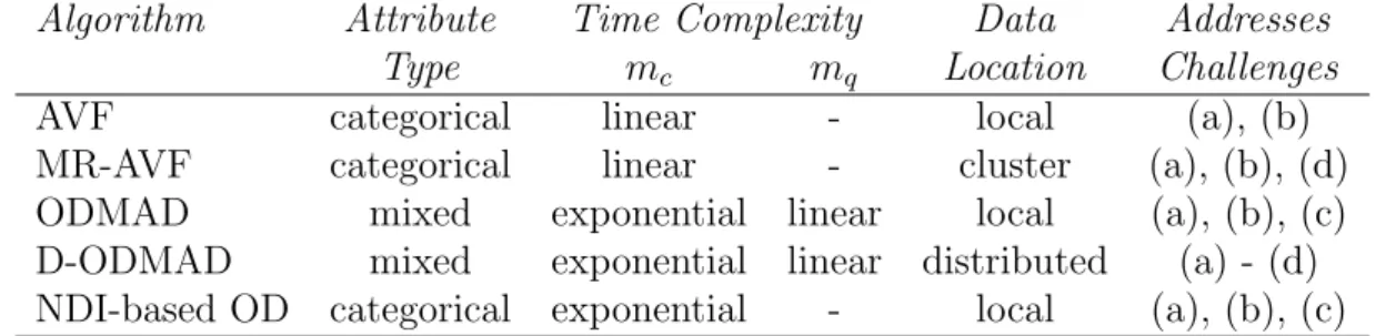
Table 1: Algorithms presented in this dissertation and their characteristics w.r.t. attribute type, time complexity for categorical (mc) and continuous
(mq) attributes, location of the dataset, and challenges they address.
Algorithm Attribute Time Complexity Data Addresses
Type mc mq Location Challenges
AVF categorical linear - local (a), (b)
MR-AVF categorical linear - cluster (a), (b), (d)
ODMAD mixed exponential linear local (a), (b), (c)
D-ODMAD mixed exponential linear distributed (a) - (d)
NDI-based OD categorical exponential - local (a), (b), (c)
Table 1 includes a list of the algorithms proposed in this dissertation and their char-acteristics as illustrated in the previous paragraphs.
The organization of this dissertation is as follows. The next chapter (Chapter 2) provides a thorough literature review of Outlier Detection algorithms. It also includes a review of Frequent Itemset Mining (FIM) and Condensed Representations of Frequent Itemsets (CFI). Chapters 3 through 6 describe the different contributions proposed in this dissertation. Finally, Chapter 7 provides a summary of our work as well as directions for future research.
CHAPTER 2
PREVIOUS WORK
In this chapter we provide an overview of the previous work in Outlier Detection, as well as a review of the work in Frequent Itemset Mining and Condensed Frequent Itemset Representations.
2.1 Outlier Detection
The existing outlier detection work can be categorized as follows: Statistical/Model-based, Distance-based and Clustering, Density-Statistical/Model-based, other approaches, and approaches for categorical and mixed-type attribute data.
2.1.1 Statistical/Model-based Approaches
Statistical outlier detection was one of the earliest approaches dating back to the 19th century [Edg87]. Statistical-based methods assume that a parametric model, which is usually univariate, describes the distribution of the data [BL78]. Multivariate statisti-cal approaches have been proposed, including use of robust (or less affected by outliers) estimates of the multidimensional distribution parameters, e.g. minimum covariance
determinant (MCD) and minimum volume ellipsoid (MVE) [Rou85, RLW87]. One in-herent problem of statistical-based methods is finding the suitable model for each dataset and application. Also, as data increases in dimensionality, it becomes increasingly more challenging to estimate the multidimensional distribution [AY01, TSK05].
As the data increases in dimensionality, data is spread through a larger volume and becomes sparse. In addition to the slowing effect this has on performance, it also spreads the convex hull, thus distorting the data distribution (“Curse of Dimensionality” [HA04]). This can be alleviated by preselecting the most significant features to work with (e.g. [AB94]), projecting to a lower-dimensional subspace [AY01]), or applying Principal Com-ponent Analysis (PCA). Another approach to deal with higher dimensionalities is to or-ganize data points in convex hull layers according to their peeling depth, based on the idea that outliers are data objects with a shallow depth value, e.g. [PS85]. In practice, however, the complexity lower bound is Ω(nm/2) forn data points andm dimensions and perform acceptably only for m≤2.
2.1.2 Distance-based and Clustering Approaches
Distance-based techniques do not make assumptions for the data since they basically compute the distance between each point. For example, Knorr et al. in [KN98] proposed a k-NN approach where, if m of the k nearest neighbors of a point are within a specific distance d, then the point can be classified as normal. Knorr et al. in [KNT00] define a point as an outlier if at least p% of the points in the dataset lie further than distance
d from it. These methods exhibit high computational complexity (e.g. nearest neighbor based methods have quadratic complexity with respect to the number of data points) which renders them impractical for really large datasets.
Several methods may be employed to make thek-NN queries faster (to achieve linear or logarithmic time), such as an indexing structure (e.g. KD-tree, or X-tree); however these structures have been shown to break down as the dimensionality grows [BS03]: for example, Breunig et al. in [BKN00] used an X-tree index and state that its performance degenerated for dimensionality ≥ 10. Bay et al. in [BS03] proposed a distance-based algorithm based on randomizing the data for efficient pruning of the search space, which in practice has complexity close to linear. This method was shown to have lower accuracy and slower performance for large data when compared to the method in [OGP06].
More recently, there have been efforts toward distance-based approaches in sub quadratic time. Angiulli et al. in [AP05] used a Hilbert Space Filling Curve to assist with
k-NN computations; however their method requires m+1 scans of the data where m
is the dataset dimensionality, which again might be impractical for distributed, high-dimensional data. Besides efficiency, a general limitation of distance-based methods is apparent in complex datasets that contain outliers which are only obvious when one looks locally at the neighborhood of each point. Distance-based methods using a global outlier criterion fail to identify these outliers.
Several clustering methods can be used (e.g. k-means, k-medoids, etc.) to form clusters, based on the idea that outliers are points not included in formed clusters. An-other idea [She02] is using a graph to reflect the connections between each and every
point, then to find the difference (distance) between a point and its neighboring points on a connected graph so that the outliers are those with distance greater than a given threshold; however this technique is applicable only in cases when a graph of the data can be constructed. In general, all the clustering-based methods rely on the concept of the clusters to define the outliers and thus they are focused in optimizing clustering, not outlier detection [KNT00].
2.1.3 Density-based Approaches
Density-based methods estimate the density distribution of the input space and then identify outliers as those lying in regions of low density. Older examples include using Gaussian Mixture Models (GMMs) e.g. [RT94]. Breunig et al. in [BKN00] assign a degree of outlier-ness to each data point, the local outlier factor (LOF), based on the local density of the area around the point and the local densities of its neighbors, relying on a user-given minimum number of points.
Extensions include Local Correlation Integral (LOCI) which uses statistical values to avoid user-entered parameters [PKG03], and using kernel density functions [LLP07]. These techniques are able to detect outliers that are missed by techniques with a single, global criterion, such as distance-based techniques [KNT00]. These methods are also based on distance computations which might be inappropriate for categorical data, and again not straightforward to implement in a distributed setting.
In addition, high-dimensional data is almost always sparse, which creates problems for density-based methods [TSK05]. In such data, the traditional Euclidean notion of density, i.e. number of points per unit volume, becomes meaningless. The increase in dimensionality leads to increase of volume, and density tends to zero as the number of dimensions grows much faster than the number of data points [ESK03]. The notion of a nearest neighbor or a similar data point does not hold as well because the distance between any two data points becomes almost identical [BGR99]. To deal with sparse data, Ertoz et al. in [ESK03] use the cosine function and shared nearest neighbors to cluster data with high dimensionality.
2.1.4 Other Approaches
Other outlier detection efforts include Support Vector methods, e.g., [TD04], and
Repli-cator Neural Networks [HHW02] among others. There has been much work related to
intrusion detection, e.g. [LEK03]. Many methods published in this area are particular to intrusion detection and cannot easily be generalized to other outlier detection areas.
Finally, a thorough survey on outlier detection can be found in [HA04], and a more recent one in [CBK09]. A review on fraud detection can be found in [KLS04].
2.1.5 Approaches for Data Sets with Categorical or Mixed-Type Attributes
Most of the techniques in the previous sections are geared toward numerical data and thus are more appropriate for numerical datasets or ordinal data that can be easily mapped to numerical values. In the case of categorical data, there is little sense in ordering categorical values, then mapping them to numerical values and computing distances, e.g., distance between values such as TCP Protocol and UDP Protocol [OGP06]. Another limitation of previous methods is the lack of scalability with respect to number of points and/or dimensionality of the dataset.
Outlier detection techniques for categorical data have recently appeared in the lit-erature. He et al. [HXD06] propose an outlier detection method based on the idea of Entropy [SPS48]. The methods in [HXH05, OGP06] use the concept of Frequent Itemset Mining (FIM) [AS94] in order to assign an outlier score to each data point based on the subsets this point contains. These techniques are presented and contrasted with our proposed method in Chapter 3.
Otey et al. in [OGP06] propose a distributed and dynamic outlier detection method for data with both categorical and continuous attributes. This method combines cate-gorical and continuous data as follows: for each set of catecate-gorical values (itemset), X, isolate the data points that contain set X, then calculate the covariance matrix of the continuous values of these points. A point is likely to be an outlier if it contains infre-quent categorical sets, or if its continuous values differ from the covariance. We present more details on this method in Chapter 5.
The aforementioned FI-based methods do well with respect to runtime performance and scalability with the tested datasets. Nevertheless, these outlier detection techniques rely on mining and using frequent sets, and will face problems with speed and memory requirements when applied to dense data or when the σ threshold is set too low. This is a well-known problem for frequent set mining and addressed in Chapter 6.
The previous work related to Frequent Itemset Mining and proposed solutions to address this issue are discussed in the next section.
2.2 Frequent Itemset Mining (FIM)
2.2.1 Association Rule Mining and Traditional FIM
Association Rule Mining (ARM) is a very popular data mining technique, which in-volves the extraction of relationships which exist among the data. Initially intended to tacklemarket basket analysis, i.e. to explore consumer trends in terms of their purchases [BMU97], ARM has been proven useful in a plethora of other applications, e.g. climate prediction [ZH04].
An association rule is an implication of the form “{diapers, milk} → {baby powder}”, which means that people who buy diapers and milk also tend to buy baby powder. Let I = {i1, i2, . . . , ir} be a set of r items in a database D. Each transaction (row) T in D is a set of items such that T ⊆ I. Given X, a set of some items in I, we say that T
abcd: 1
abc: 3 abd: 2 acd: 1 bcd: 1
ab: 4 ac: 3 ad: 3 bc: 3 bd: 2 cd: 1
a: 5 b: 4 c: 3 d: 3
Frequent
Infrequent
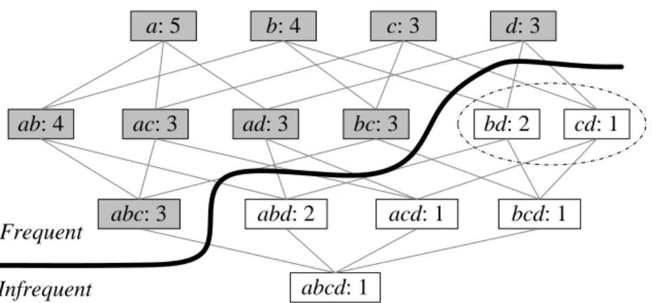
Figure 2: Example of Frequent Sets, Infrequent Sets, and Sets on Negative Border
D that contain X. We say that X is frequent if it appears at least σ times in D, where
σ is a user-defined threshold.
A set X belongs in the negative border of the frequent sets, if all subsets of X are frequent butXitself is infrequent. Figure 2 depicts an example dataset with the resulting frequent sets and negative border sets. For example, set bd is on the negative border, but set abdis not, as it contains a subset bd that is infrequent.
Given a minimum threshold σ, mining of association rules contains two distinct phases: (a) find frequent itemsets, i.e. those with frequency no less than σ, and (b) generate the confident, or interesting rules which contain the frequent itemsets. The first problem of finding the frequent itemsets, which is referred to as Frequent Itemset Mining (FIM), has been identified as the most complex of the two.
The main idea behind all algorithms for mining frequent (or large) itemsets, can be described as follows: in the first pass over the data, count the support of individual items, and determine which have minimum support (large or frequent). Then, in the next data
pass, use only those itemsets that were found to be large or frequent in the previous pass, in order to generate new potentially large itemsets, calledcandidate itemsets, and count the support for these candidate itemsets. The frequent candidate itemsets, i.e. those that pass the minimum support threshold, are used to construct the candidate itemsets for the next pass, and so on. This loop ends when no new large itemsets can be found.
Agrawal and Srikant introduced the first efficient FIM algorithm, called Apriori [AS94]. The difference between the Apriori algorithm and the prior research is in the way it generates the aforementioned candidate itemsets, and also in the way the candidates are counted in each pass. Apriori’s central property is: “If A is a frequent itemset, then every subset of A is a frequent itemset”. What ensues from this statement is that, once a set has been found infrequent, not only can it be pruned, but all the itemsets that contain it can be pruned as well, as they are also infrequent. For example, if set ab has been found to be infrequent, then itemsetsabc,abe,abce, etc., that contain setab, cannot be frequent, so they too can be pruned.
There are several algorithms in the literature to improve different aspects of Apriori, e.g.: DIC [BMU97], which dynamically counts candidates of varying length to reduce number of scans; DHP [PCY95], which collects approximate counts to rule out candidates that cannot possibly be frequent; FP-Growth [HPY04], which stores the transactions in an FP-tree, a trie structure where every item contains a list of all the transactions that contain that item. Also there are several ARM implementations online [Bod03, Bor03, Goe05].
2.2.2 Condensed Representations of FIs (CFIs)
Apriori-inspired algorithms perform well with sparse data sets, such as market-basket data, where the frequent patterns are short, but they face problems for dense data. Even with candidate pruning in Apriori, the resulting frequent itemsets might still be numer-ous, an issue exacerbated when these sets contain millions of items or the σ threshold is too low. The problems that FIM algorithms face with such data is not due to design or implementation of the specific FIM algorithm, but the large number of FIs that are generated.
To solve this issue much work has been conducted towardCondensed Representations of FIs (CFIs) e.g. [AAP00, ZH05, CG07]. The goal of these methods is to find a much smaller group of representative sets, from which one can deduce all FIs. Many CFIs have been proposed, which we briefly describe next (more details can be found in [CRB04]).
A maximal set is a frequent set that is not a subset of any other frequent itemset [AAP00]. Aclosed set is a set with support such that there is no superset with support equal to it [PBT99]. LetM be the set of maximal sets and C the set of closed sets. Even though in theoryM andC can be exponential in the number of items, in practice,C can be orders of magnitude smaller than the number of frequent sets (especially for dense data), while M can be orders of magnitude smaller than C.
Closed sets are lossless in the sense that the exact frequency of all FIs can be de-termined from C, while M leads to a loss of information (since subset frequency is not kept)[ZH05]. Once a given support threshold is known as well as all frequent closed
itemsets with their supports, the rest of the frequent itemsets and their supports can be generated. If an itemset I has at least one superset in the set of all frequent closed item-sets (FreqClosed), then the supp(I) = supp(cl(I)) where cl(I) is the smallest superset of I in FreqClosed. The reader is reminded that the Apriori Principle states that if an itemset is frequent, then all of its subsets are frequent. Thus, the itemset I in this case is frequent.
δ-free sets [BBR00] can be used as a δ-adequate representation for FIs. If we know that the association rule abc→ d is nearly an exact rule (i.e. it is true for “most” of the dataset), we can approximate the frequency of set abcd using the frequency of abc. A
δ-strong rule is an association rule of the form X ⇒δ a, where X ⊆ I, a ∈ I\X, and δ is a natural number. The rule is valid if it is not violated in more than δ transactions. An itemsetY isδ-free if there is no validδ-strong rule X ⇒δa such that X ⊂Y,a∈Y, and a /∈ X. Given any database D, the set of all frequent δ-free sets can be used to approximate the support of the frequent non-δ-free sets [BBR00].
The authors in [CG07] propose determining bounds on the support of an itemset I, based on the supports of subsets of I. An itemset I is called derivable when its support can be exactly deduced from the support of its subsets [CG07]. Derivable itemsets repre-sent redundant information and can be pruned, so that Non-Derivable Itemsets (NDIs) can form a condensed representation. NDIs have been shown to be significantly more concise than the complete FI collection, and in many cases smaller than the previously mentioned representations [CG05].
2.2.3 Other methods
Besides condensed representations, other types of patterns have been proposed and used as a step prior to a data mining tasks such as clustering. For example, [XPS06] used highly-correlated association patterns called hyperclique patterns [XTK06] as a cleaning step to filter out noisy objects, resulting in better clustering performance and higher quality associations. The authors in [HXY07] use hyperclique patterns to detect off-topic documents. The authors in [WK06] proposed summary sets in an effort to summarize categorical data for clustering; summary sets were proven to be closed sets. Finally, in [JC08] a support approximation and clustering method was proposed to mine FIs in the dataset.
CHAPTER 3
OUTLIER DETECTION FOR CATEGORICAL DATA:
ATTRIBUTE VALUE FREQUENCY (AVF)
3.1 Introduction
In this chapter, we introduce an fast outlier detection strategy for categorical data, called Attribute Value Frequency (AVF) [KOG07]. We compare AVF with existing outlier de-tection methods with respect to runtime performance as well as outlier dede-tection accuracy. These previous efforts have not been contrasted to each other using the same datasets.
The first method by He et al. [HXD06] is an outlier detection method based on the idea of Entropy. The second technique by Otey et al. [OGP06] focuses on datasets with mixed attributes (both categorical and numerical). The third technique is by He et al. [HXH05]. Both methods in [HXH05, OGP06] compute an outlier score for each data point using the concept of Frequent Itemsets [AS94].
Wei et al. [WQZ03] also deal with outliers in categorical datasets using frequent itemsets, as well. In fact, they use hyperedges to store frequent itemsets and the data points that contain these frequent itemsets; since their method is similar to that in [HXH05], it was not considered in our experiments. Finally, Yu et al. [YQL06] use mutual reinforcement to discover outliers in a mixed attribute space; however their method focuses on a different outlier detection problem than the one described in this dissertation
(“instead of detecting local outliers as noise, [they] identify local outliers in the center, where they are similar to some clusters of objects on one hand, and are unique on the other.” [YQL06]).
Experimentation with real and artificial data sets show that AVF has a significant performance advantage, and scales linearly as the data set increases in number of points and number of dimensions. In addition, AVF is efficient for large and geographically distributed data sets as it performs only one dataset scan.
3.2 Greedy Algorithm
The algorithms in [HXD06] are based on the assumption that outliers are likely to be the points that the dataset as a whole has less “uncertainty” or “disorder” if these outliers are removed from the data. In particular, they propose to identify a small subset (of size
k) of the data points which contribute the most to the “disorder” of the dataset. The idea of Entropy, or uncertainty, of a random variable is attributed to Shannon [SPS48]. Formally, if X is a random variable,S(X) is the set of values thatX can take, and p(x) is the probability function ofX, the entropy, E(X), is defined as follows:
E(X) =− X x∈S(X)
p(x) log2p(x) (3.1)
GivenX ={X1, X2, . . . , Xm}, a dataset containingmattributes, and the assumption
Input : Database D (n points × m attributes), Target number of outliers - k
Output: k detected outliers
Label all data points as non-outliers;
1
foreach point xi, i= 1. . . n do
2
foreach attribute l, l = 1. . . m do
3
Count frequencyf(xil) of attribute value xil;
4
end
5
end
6
Calculate initial Entropy of dataset, E;
7
while not k scans do
8
foreach normal point xi, i= 1. . . n do
9
xi ←outlier;
10
∆i := decrease in entropy E by removing xi;
11
end
12
if decrease ∆i is max then
13
Addxi to set of k outliers;
14
end
15
end
16
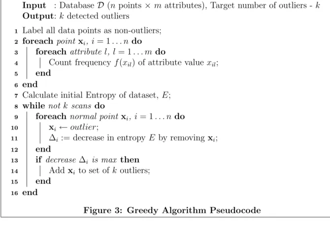
Figure 3: Greedy Algorithm Pseudocode
of the entropies of each one of the m attributes, and is defined as follows:
E(X) = E(X1) +E(X2) +. . .+E(Xm) (3.2)
He et al. introduce a Local-Search heuristic-based Algorithm (LSA) in [HDX05], and a Greedy Algorithm in [HXD06] both relying on the entropy idea mentioned above. Since the Greedy algorithm is superior to LSA, we will only discuss the Greedy algorithm. The Greedy algorithm takes as input the desired number of outliers (k). All points in the set are initially designated as non-outliers. At the beginning, the frequencies of all attribute values are computed, as well as the initial entropy of the dataset.
Then, Greedy conducts k scans over the data to determine the top k outliers. Dur-ing each scan, every non-outlier is temporarily removed from the dataset and the total
entropy is recalculated. The non-outlier point that results in the maximum decrease for the entropy of the entire dataset is the outlier data-point removed by the algorithm in each scan. Pseudocode for Greedy is provided in Figure 3.
The complexity of Greedy isO(k×n×m×q) , wherekis the target number of outlier points, n designates the number of points in the dataset, m is the number of attributes, andq is the number of distinct attribute values, per attribute. If the number of attribute values per attribute, q, is small, the complexity of Greedy becomes O(k×n×m).
3.3 FindFPOF
Frequent Itemset Mining (FIM) was introduced in the Literature Review Section 2.2. He et al. in [HXH05] observe that, since frequent itemsets are “common patterns” that are found in many of the points of the dataset, outliers are likely to be the points that contain very few common patterns or subsets. They define a Frequent Pattern Outlier Factor (FPOF) for every data point, x, based on the support of the frequent itemsets contained in x. In addition, they use a contradictness score to better explain the outliers and not to detect the outliers, so it is omitted from our discussion. The FPOF outlier score is calculated as follows:
F P OF Score(xi) =
X
F⊆xi∧F∈F I
supp(F)
Input : Database D (n points ×m attributes), Target number of outliers - k, minimum support σ
Output: k detected outliers
Label all data points as non-outliers;
1
F I = Get all frequent itemsets(D, σ);
2 foreach point xi, i= 1. . . n do 3 foreach F ⊆xi∧F ∈F I do 4 F P OF Score(xi) += supp(F); 5 end 6 F P OF Score(xi) /= |F I|; 7 end 8
Return k outliers with mini(F P OF Score);
9
Figure 4: FindFPOF Pseudocode
The above score is the sum of the support of all the frequent subsets F contained in point xi, over the total number of frequent sets in dataset D, |F I|. Data points with lower FPOF scores are likely to be outliers since they contain fewer common subsets. The FPOF algorithm runs a FIM algorithm such as Apriori [AS94] first, to identify all frequent itemsets in datasetD given thresholdσ, then calculates the FPOF outlier score for each data point, to identify the top k outliers (see pseudocode in Figure 4).
3.4 Otey’s Method for Categorical Data
The method by Otey et al. in [OGP06] is also based on frequent itemsets. They assign to each point an anomaly score inversely proportional to its infrequent itemsets. They also maintain a covariance matrix for each itemset to handle continuous attributes; we omit this part since our focus is on categorical data.
Input : Database D (n points ×m attributes), Target number of outliers - k, minimum support σ
Output: k detected outliers
Label all data points as non-outliers;
1
F I = Get all frequent itemsets(D, σ);
2 foreach point xi, i= 1. . . n do 3 foreach possible I ⊆xi∧I /∈F I do 4 OteyScore(xi) += 1/|I|; 5 end 6 end 7
Return k outliers with maxi(OteyScore);
8
Figure 5: Otey’s Pseudocode (Categorical Data)
Specifically, they calculate the following score for each data point xi:
OteyScore(xi) =
X
d⊆xi∧d /∈F I 1
|d| (3.4)
which is explained as follows: given subsets d of xi which are infrequent, i.e. support of
d is less than σ, the anomaly score of xi will be the sum of the inverse of the length of
d. If a point has few frequent itemsets, its outlier factor will be high, so the outliers are the k points with the maximum outlier score in Equation (3.4). This algorithm also first mines the data for FIs, then calculates an outlier score for each point (see pseudocode in Figure 5). The authors state that the execution time is linear to the number of data points, but exponential to the number of categorical attributes.
3.5 Attribute Value Frequency (AVF)
The algorithms discussed so far do scale linearly with respect to the number of data points, n. However, Greedy (section 3.2) still needs k scans over the dataset to find k
outliers, a disadvantage for the case of very large datasets that are potentially distributed among different sites. On the other hand, the Frequent Itemset Mining (FIM)-based approaches (sections 3.3 and 3.4) need to create a potentially large space of subsets or itemsets, and then search for these sets in each and every data point. These techniques can become extremely slow for low values of theσ threshold, as more and more candidate itemsets need to be examined.
In this section we present a simpler and faster approach to detect outliers that min-imizes the scans over the data and does not need to create or search through different combinations of attribute values or itemsets. We call this outlier detection algorithm Attribute Value Frequency (AVF) algorithm.
It is intuitive that outliers are those points which are infrequent in the dataset. Ad-ditionally, an ideal outlier point in a categorical dataset is one whose each and every attribute value is extremely irregular (or infrequent). The infrequent-ness of an attribute value can be measured by computing the number of times this value is assumed by the corresponding attribute in the dataset.
Lets assume that the dataset containsn data points,xi, i= 1. . . n. If each data point has m attributes, we can write xi = [xi1, . . . , xil, . . . , xim], where xil is the value of the
Data Attributes point 1 2 3 4 5 6 7 8 9 1 1 1 1 1 2 10 3 1 1 2 2 1 1 1 2 1 2 1 1 3 1 1 1 1 2 3 3 1 1 4 4 1 1 1 2 1 2 1 1 5 4 1 1 1 2 1 3 1 1 6 6 1 1 1 2 1 3 1 1 * 7 7 3 2 10 5 10 5 4 4 8 3 1 1 1 2 1 2 1 1 9 1 1 1 1 2 1 3 1 1 10 3 2 1 1 1 1 2 1 1 11 5 1 1 1 2 1 2 1 1 * 12 2 5 3 3 6 7 7 5 1
Figure 6: Example of normal and outlier points from UCI Breast Cancer Dataset. Outlier points are denoted by asterisk.
decide if point xi is an outlier can be defined as the AVF Score below:
AV F Score(xi) = 1 m m X l=0 f(xil) (3.5)
wheref(xil) is the number of times the l-th attribute value of xi appears in the dataset. Since we essentially have a sum ofmpositive numbers, the AVF score is minimized when each of the summation terms are individually minimized. Thus, the AVF score will be minimum for the ‘ideal’ outlier as defined earlier.
Figure 6 contains an example with 12 points taken from UCI [BM98] Breast Cancer dataset. The outliers are denoted by an asterisk (points 7 and 12). As this example clearly illustrates, the outliers have infrequent values for all or most of the 9 attributes, compared to the rest of the data points.
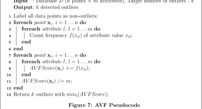
Once we calculate the AVF score of all the points, we designate the k points with the smallest AVF scores as thekoutliers (see Figure 7 for AVF pseudocode). The complexity
Input : Database D (n points × m attributes), Target number of outliers - k
Output: k detected outliers
Label all data points as non-outliers;
1
foreach point xi, i= 1. . . n do
2
foreach attribute l, l = 1. . . m do
3
Count frequencyf(xil) of attribute value xil;
4 end 5 end 6 foreach point xi, i= 1. . . n do 7 foreach attribute l, l = 1. . . m do 8 AV F Score(xi) += f(xil); 9 end 10 AV F Score(xi) /= m; 11 end 12
Return k outliers with mini(AV F Score);
13
Figure 7: AVF Pseudocode
of AVF is O(n×m) compared to Greedys complexity, O(k×n×m), since AVF detects outliers after only one scan of the dataset, instead of the k scans needed by Greedy.
3.6 Experiments
3.6.1 Experimental Setup
We conducted all our experiments on a workstation with a Pentium 4 2.6 GHz processor and 1.5 GB of RAM. We implemented all algorithms in C++ and ran our own implemen-tation of Apriori [AS94] for mining frequent itemsets for FPOF and Otey’s algorithms (σ = 10%). We experimented with 5 real datasets from the UCI Machine Learning repository [BM98], as well as artificially generated datasets (described in Appendix B).
An advantage of using artificially generated data is the capability to work with datasets of various sizes and dimensionalities.
The experiments conducted with the simulated data were used to showcase the speed and associated scalability of the algorithms that we are evaluating, and not their de-tection rates/capabilities (effectiveness). The simulated datasets used are described in Appendix B. The idea behind these experiments is to see the change of each algorithm’s performance as parameters change (e.g., an important parameter is the size of the dataset,
n and the dataset dimensionality, m). For example, Greedy calculates the Entropy for each dimension of each data point. Finally, it is worth mentioning that the runtime of the Greedy algorithm also depends on the input number of outliers, k, while the other algorithms do not.
For the first experiment we used a dataset with 10 attributes and input number of outliers,k=30, and 1K to 800K data points. For the second experiment, the dataset has 100K points and 10 attributes, and the outlier target numberk varies from 1 to 1K. For the last experiment, the outlier number k is set to 30, the dataset contains 100K points, and the number of attributes is varied from 2 to 40.
3.6.2 Results and Discussion
Table 2 depicts the outliers detected by each algorithm using the real datasets. As we see in the experiments with the real datasets, the outlier detection accuracy of AVF is the same as, or very close to Greedy. For example, in Table 2(a), all algorithms converge to
the 39 outliers forkequal to 56. While we notice similar accuracy in detecting outliers for all algorithms for the breast cancer, lymphography, and post-operative patients datasets (Table 2(a)-(c)), for the other two datasets (Table 2(d)-pageblocks and Table 2(e)-adult), AVF has lower accuracy than Greedy, while FPOF and Otey’s have much lower accuracy (e.g. in Table 2(d) fork=900 Greedy detects 242 outliers, AVF detects 223, while FPOF and Otey’s detect only 116).
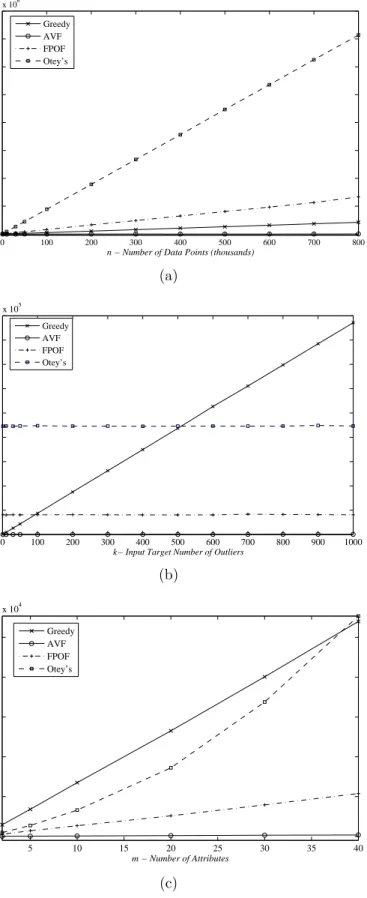
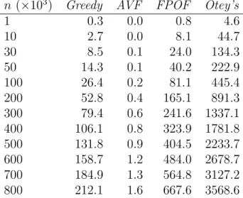
Table 3 contains the runtime performance of all algorithms using the first simulated dataset, with varying number of data points, n (see also Figure 8(a)). For example, in Table 3, for n=700K, Greedy finishes execution at around 185 seconds, Otey’s methods at around 3127 seconds, FPOF at 564 seconds, while AVF has a running time of 1.33 seconds. Further experiments with larger dimensionalities than the ones in Figure 8(c) showed that AVF is still much faster, e.g. for a dataset with n=100K andm=100, AVF had a running time of about 1.36 seconds (k = 30).
As we see from these results with real and artificially generated data, AVF approx-imates very well the outlier detection accuracy of Greedy, while it outperforms Greedy for larger values of the data size, n, data dimensionality, m, and the target number of outliers,k. E.g., Greedy becomes exceedingly slow for larger n values (Figure 8(a)), due to the increasingly more expensive entropy calculations. The performance of AVF does not change notably for larger k values, and it runs significantly faster than Greedy with respect to both n and m, as AVF relies on simple calculations for each point.
The FIM-based methods also become increasingly slower for larger datasets (see Fig-ure 8(a)), as they need to search through all possible subsets of each and every point.
Table 2: AVF, Greedy, FPOF, and Otey’s Accuracy Results on Real Datasets
(a) Breast Cancer
k Greedy AVF FPOF Otey’s
4 4 4 3 3 16 15 14 14 15 24 22 21 21 21 32 29 28 27 28 48 37 36 35 37 56 39 39 39 39 (b) Lymphography
k Greedy AVF FPOF Otey’s
2 2 2 2 2 4 4 4 4 4 6 5 4 4 4 8 6 5 5 5 12 (13) 6 6 5 5 (6) 15 6 6 6 6 (c) Post-Operative
k Greedy AVF FPOF Otey’s
10 4 3 3 1 20 7 7 7 7 30 8 10 9 9 40 12 11 10 10 60 20 16 17 18 80 24 24 24 24 (d) Pageblocks
k Greedy AVF FPOF Otey’s
100 45 40 19 19 200 81 84 42 42 300 130 120 63 63 500 177 189 80 80 800 237 214 110 110 900 242 223 116 116 1000 242 233 121 121 (e) Adult
k Greedy AVF FPOF Otey’s
100 24 27 21 16
200 41 45 42 37
400 87 88 82 66
600 124 116 114 96
0 100 200 300 400 500 600 700 800 0 0.5 1 1.5 2 2.5 3 3.5 4x 10 6
n − Number of Data Points (thousands)
Time (milliseconds) Greedy AVF FPOF Otey’s (a) 0 100 200 300 400 500 600 700 800 900 1000 0 1 2 3 4 5 6 7 8 9x 10 5
k− Input Target Number of Outliers
Time (milliseconds) Greedy AVF FPOF Otey’s (b) 5 10 15 20 25 30 35 40 0 2 4 6 8 10 x 104 m − Number of Attributes Time (milliseconds) Greedy AVF FPOF Otey’s (c)
Figure 8: AVF, Greedy, FPOF, and Otey’s runtime performance for simulated data as n, k, and m increase (milliseconds).
Table 3: Runtime of AVF, Greedy, FPOF, and Otey’s Approaches in seconds for the simulated data with varying number of data points, n.
n (×103) Greedy AVF FPOF Otey’s
1 0.3 0.0 0.8 4.6 10 2.7 0.0 8.1 44.7 30 8.5 0.1 24.0 134.3 50 14.3 0.1 40.2 222.9 100 26.4 0.2 81.1 445.4 200 52.8 0.4 165.1 891.3 300 79.4 0.6 241.6 1337.1 400 106.1 0.8 323.9 1781.8 500 131.8 0.9 404.5 2233.7 600 158.7 1.2 484.0 2678.7 700 184.9 1.3 564.8 3127.2 800 212.1 1.6 667.6 3568.6
Higher dimensionalities of the datasets slow down these two algorithms as well, because of the increasingly larger itemsets that are created as the number of attributes grows (see Figure 8(c)). The authors in [OGP06, HXH05] discussed using a parameter for the maximum length of itemsets; for example, if the user enters 5 as the max length, the itemsets created contain 5 items or less. However, experiments in [OGP06] show that this might negatively affect their algorithmic accuracy.
In addition, the algorithms based on Frequent Itemsets, specifically FPOF and Otey’s, depend on the user-entered minimum support threshold. In fact, different values of σ
lead to improved accuracy of FPOF and Otey’s. For example, using the pageblocks data and k=200 (see Table 2(d)), Otey’s method with σ=0.04 detected 120 outliers, while for
σ=0.03, it detects 51 outliers. This is because lower σ values will create more frequent sets, while higher σ values will make more subsets infrequent. Also, lowerσ values make the algorithms increasingly slower as more frequent itemsets need to be created. This illustrates the challenge of selecting an appropriate σ.
The advantages of AVF are that it does not create itemsets and that it entails only a single pass over the entire dataset. Also, as shown from the experiments with the simulated datasets, the runtime of AVF increases particularly slowly with respect to n
and m, in comparison to the other three algorithms. Moreover, AVF eliminates the need for difficult choices for any user-given parameters such as minimum support or maximum itemset length. However, experimentation with some small datasets showed that the single scan of the data may cause AVF to miss a few outliers that Greedy finds. This effect was negligible in the real datasets with which we experimented in this chapter. The next chapters deal with ways to increase the outlier detection accuracy of AVF, but at the expense of decreasing its efficiency (speed).
3.7 Summary
We have compared and experimented with a representative list of available methods for detecting outliers in categorical datasets, using both real-world and artificially generated data. These methods have not been compared against each other before using the same datasets. We have proposed a scalable and effective outlier detection technique, called Attribute Value Frequency (AVF). AVF lends itself to the nature of datasets today, as its performance does not deteriorate given datasets with a large number of data points and/or large number of dimensions.
• A computational complexity of O(n×m), where n is the number of points in the data, and m is the data dimensionality, i.e. it scales linearly with both n and m;
• The performance of AVF does not depend on additional user-entered parameters, such as minimum support (σ);
• AVF needs one dataset scan to detect the desired outliers; also, the number of data scans needed by AVF does not rely on the input number of target outliers (k);
• AVF runs significantly faster than the existing representative techniques, while maintaining comparable detection accuracy.
CHAPTER 4
PARALLEL OUTLIER DETECTION FOR CATEGORICAL
DATASETS USING MAPREDUCE: MR-AVF
4.1 Introduction
As mentioned in the previous Chapter, AVF is based on assigning a score to each point in the dataset using the frequency of each unique attribute value, thus it is easily par-allelizable. In contrast, other techniques for outlier detection in categorical data (see [OGP06, HXH05]) are much more complicated and cumbersome to parallelize, as they require several scans of the dataset, in order to extract frequently encountered, and sometimes lengthy, combinations of attribute values.
In this chapter, we introduce MapReduce-AVF (MR-AVF) [KSR08], a parallel out-lier detection method for categorical datasets, geared toward identifying outout-liers in large data mining problems. MR-AVF is based on the MapReduce paradigm of parallel pro-gramming [DG04]. MapReduce provides the necessary simplicity of parallel development, while it guarantees load balancing and fault tolerance for the implementation. It is worth noting that MapReduce has already been successfully used in parallelizing a number of machine learning approaches for data mining applications (e.g., see [CKL07]).
MR-AVF is based on AVF, which has been shown to perform favorably compared to other competitive but more complex outlier detection strategies. Due to its simplicity,
AVF is an ideal method to parallelize, and using the MapReduce approach to parallelize it guarantees ease of development, load balancing and fault tolerance of the implementation. Our results show that MR-AVF exhibits close to ideal speedup with respect to number of processing nodes in the cluster.
The organization of this chapter is as follows: first, we provide a synopsis of the earlier work based on the MapReduce paradigm. Then, we review the MapReduce paradigm, and finally we introduce our proposed algorithm for parallel outlier detection, i.e. the MapReduce-AVF, and present our experimental results.
4.2 Background on MapReduce
MapReduce [DG04] is a simplified parallel program paradigm for large scale, data inten-sive, parallel computing jobs. MapReduce hides the parallel machine from the program-mer by simplifying the parallel programming model to two functions: the map function and the reduce function. Given a list of keys and associated values, the map function produces an intermediate set of keys and values. The reduce function then combines these intermediate values into a final result.
MapReduce has already found its way into several machine learning and data mining applications. Chu et al. [CKL07] present many algorithms in MapReduce form, in-cluding Locally Weighted Linear Regression, k-means, Logistic Regression, Naive Bayes, Linear Support Vector Machines, Independent Component Analysis, Gaussian Discrimi-nant Analysis, Expectation Maximization, and Backpropagation.
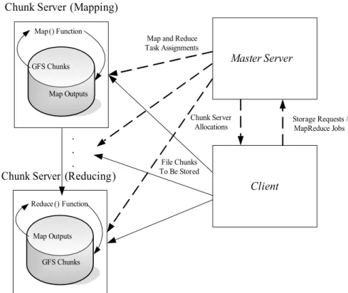
The central focus of MapReduce is to simplify the processing of large datasets on inex-pensive cluster computers. These cluster computers often contain hundreds or thousands of nodes that both store and process the datasets in a distributed fashion. Typically, a single master server is used to schedule the data storage and computation on the nodes. The original MapReduce system was built on the Google File System (GFS) [GGL03], which is optimized for storing large, infrequently changed datasets across standard disks on the cluster nodes. The MapReduce/GFS combination is built to tolerate regular node failures through replication of the data and speculative execution. This system also automatically provides for load balancing and scheduling associated with the parallel processing of the data.
Users design a MapReduce program by relying, almost entirely, on the map and reduce functions. As a consequence, the user is not forced to devise a parallelization strategy for the task at hand, but is only required to adapt it to a MapReduce model. The map function takes as input a set of key-value pairs, designated ask1 andv1, provided directly
from the user-defined input files. Within the map function, the user specifies what to do with these keys and values. The map function outputs another set of keys and values, designated as k2 and v2. The reduce function sorts the key value pairs byk2. All of the
associated valuesv2 are reduced and emitted as value v3. The map and reduce functions
are as follows:
map(k1, v1)→(k2, v2)[]
At the MapReduce run-time level, the map operations are distributed by the master-server to the chunk-master-servers. The scheduler makes an effort to schedule computation on the same node where the data is stored. Meanwhile, other chunk-servers assigned to the reduce phase begin to take the (k2, v2) value pairs and sort them by k2. These sorted
arrays of v2 values are passed to the reduce functions on these same assigned nodes.
These outputs are finally saved on the GFS. It is quite common for an application to string together many simpler MapReduce operations.
Fault tolerance and load balancing are automatically provided by the software that supports MapReduce and the GFS. Because the GFS stores a user-specified number of copies (usually three) for each chunk of the data on different chunk servers, and because the GFS monitors the cluster to maintain these copies, losing a particular chunk of data should be relatively rare. For fault tolerance of the MapReduce operations, the master server keeps track of all running operations and can re-start failed tasks on other chunk servers that have a copy of the data. By the nature of operations that are put into the MapReduce framework (map operations that are independent on each element) they can be recomputed by any chunk server with the proper data.
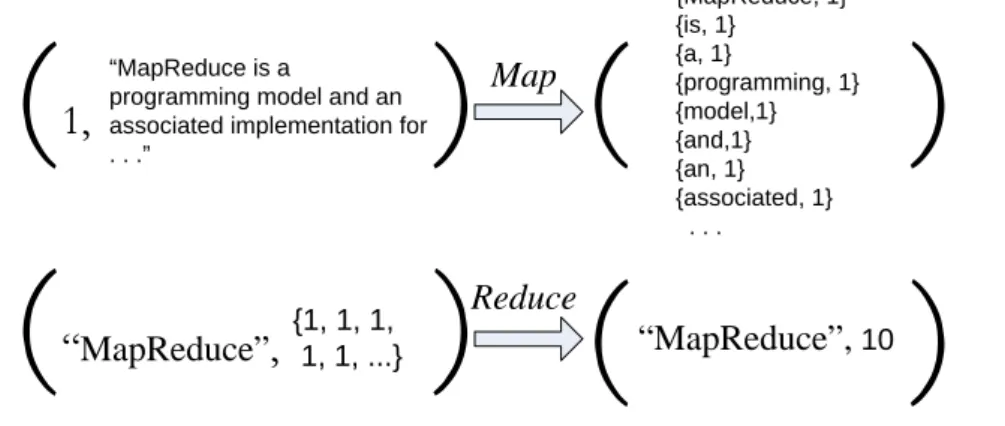
A diagram of a typical MapReduce/GFS architecture is displayed in Figure 9. An often cited MapReduce example is known as WordCount [DG04]. Suppose we need to obtain the number of occurrences of each unique word in a large file. In the MapReduce paradigm, this computation can be done easily and efficiently as follows: the map function receives as input a line from the large input file. Then the map function
Chunk Server (Mapping)
GFS Chunks
Map Outputs Map () Function
Master Server
Chunk Server (Reducing)
GFS Chunks Reduce () Function Map Outputs Client Storage Requests / MapReduce Jobs Chunk Server Allocations . . . File Chunks To Be Stored Map and Reduce Task Assignments
Figure 9: The flow of data in a MapReduce/GFS architecture for file storage and MapReduce operations (dashed lines indicate control messages, and solid lines indicate data transfer).
1,
“MapReduce is a
programming model and an associated implementation for . . .” {MapReduce, 1} {is, 1} {a, 1} {programming, 1} {model,1} {and,1} {an, 1} {associated, 1} . . . Map
“
MapReduce”,
{1, 1, 1, 1, 1, ...} “MapReduce”, 10 ReduceFigure 10: A pictorial illustration of the WordCount example.
splits this line into its component words and emits the word as the key and ‘1’ as the associated value.
The reduce function takes the word-keys and ‘1’ values as input. Each ‘1’ value is an occurrence of the corresponding word, so the reduce function sums the values to find the number of occurrences of the word. When the reduction operation is complete, there is a list of words with their associated occurrence frequency. See Figure 10 for a pictorial illustration of the WordCount example.
4.3 MR-AVF
Using MapReduce, the Map function associates each distinct attribute value to the Map’s output key. The Reduce function computes the frequency counts of each attribute value. Finally, the AVF score of each data point is calculated during a second Map function. The second Reduce is simply a sorting operation of the computed AVF scores.
Input : Database D (n points × m attributes), Target number of outliers - k
Output: k detected outliers HashTable H; 1 map k1 =i, v1 =Di =xi, i= 1. . . n begin 2 foreach l∈xi, l= 1. . . m do 3 collect(xil, 1); 4 end 5 end 6 reduce k2 =xil, v2 begin 7 H(xil) +=v2; 8 end 9 map k1 =i, v1 =Di =xi begin 10 AV F = m X l=1 H(xil); 11 collect(k1,AV F); 12 end 13 reduce k2 =AV Fi, v1 =i; 14
Figure 11: MR-AVF Pseudocode
The pseudocode for MapReduce-AVF, MR-AVF, is depicted in Figure 11. In the first pair of Map/Reduce functions (first phase, lines 2-9), the frequency of each attribute value is extracted from the data set. If the attribute values across each attribute are unique or the dimension is concatenated to the attribute value (as in our code), this pair of functions is similar to the WordCount problem described in the previous section.
In the second MapReduce phase (lines 10-14), the attribute value frequency table resulting from the first phase is loaded into the hash tableH by the map function. The map function then calculates and emits the AVF score for each individual input record, by iterating through the dimensions and adding the frequency of every attribute value. In order to sort the data points by their outlier score, the AVF score is emitted as the key, and the input point ID is emitted as the value.
At the end of the MapReduce process, the result is a list of AVF scores sorted in ascending order with the listed point IDs. As a result, the top-k