Virginia Commonwealth University
VCU Scholars Compass
Theses and Dissertations Graduate School
2015
A Study on False Information Injection Attack on
Dynamic State Estimation in Multi-Sensor Systems
Jingyang Lu
[email protected]Follow this and additional works at:http://scholarscompass.vcu.edu/etd Part of theSystems and Communications Commons
© The Author
This Thesis is brought to you for free and open access by the Graduate School at VCU Scholars Compass. It has been accepted for inclusion in Theses and Dissertations by an authorized administrator of VCU Scholars Compass. For more information, please [email protected].
Downloaded from
©
Jingyang Lu 2015 All Rights Reserved
A Study on False Information Injection Attack on
Dynamic State Estimation in Multi-Sensor Systems
A thesis submitted in partial fulfillment of the requirements for the degree of Master of Science at Virginia Commonwealth University
by Jingyang Lu
Adviser: Ruixin Niu
Department of Electrical and Computer Engineering
Virginia Commonwealth University Richmond, Virginia
CONTENTS
I Abstract iii
II Introduction 1
III Kalman Filter System 3
III-A Linear Dynamic State Estimation . . . 3 III-B The Recursive Estimation Algorithm . . . 4 III-C Statistical Test for Filter Consistency . . . 6
IV System Model 7
V Impact of False Information Injection 8
VI The Optimal Attack Strategy 10
VI-A Problem Formulation for a General Linear System . . . 10 VI-B Equivalent Measurement in Multi-Sensor Systems . . . 10
VII A Target Tracking Example 13
VII-A Attack Strategy Analysis from Trace Perspective . . . 13 VII-A1 Attack Strategy for Multiple Position Sensors . . . 13 VII-A2 Attack Strategy for a Single Position and Velocity Sensor . . . 16 VII-A3 Attack Strategy for Multiple Position and Velocity Sensors . . . 20 VII-A4 Strategy for a Single Sensor with Multiple Time Attacks . . . . 22 VII-B Attack Strategy Analysis from Determinant Perspective . . . 24 VII-B1 Attack Strategy for Multiple Position Sensors . . . 24 VII-B2 Attack Strategy for a Single Position and Velocity Sensor . . . 25 VII-B3 Attack Strategy for Multiple Position and Velocity Sensors . . . 29
VIII Numerical Results 31
VIII-A Systems with Position Sensors . . . 31 VIII-B Systems with Position and Velocity Sensors . . . 31 VIII-C Determinant Case . . . 33
IX Conclusion 38
Abstract
A STUDY ON FALSE INFORMATION INJECTION ATTACK ON DYNAMIC STATE ESTIMATION IN MULTI-SENSOR SYSTEMS
By Jingyang Lu, Master
A thesis submitted in partial fulfillment of the requirements for the degree of Master of Science at Virginia Commonwealth University.
Virginia Commonwealth University, 2015. Major Director: Ruixin Niu
In this thesis, the impact of false information injection is investigated for linear dynamic systems with multiple sensors. It is assumed that the Kalman filter system is unaware of the existence of false information and the adversary is trying to maximize the negative effect of the false information on the Kalman filter's estimation performance. First, a brief introduction to the Kalman filter is shown in the thesis. We mathematically characterize the false information attack under different conditions. For the adversary, many closed-form results for the optimal attack strategies that maximize the Kalman filter's estimation error are theoretically derived. It is shown that by choosing the optimal correlation coefficients among the bias noises and allocating power optimally among sensors, the adversary could significantly increase the Kalman filter's estimation errors. To be concrete, a target tracking system is used as an example in the thesis. From the adversary's point of view, the best attack strategies are obtained under different scenarios, including a single-sensor system with both position and velocity measurements, and a multi-sensor system with position and velocity measurements. Under a constraint on the total
power of the injected bias noises, the optimal solutions are solved from two perspectives: trace and determinant of the mean squared error matrix. Numerical results are also provided in order to illustrate the negative effect which the proposed attack strategies could inflict on the Kalman filter.
II. INTRODUCTION
System state estimation in the presence of an adversary that injects false information into sensor readings is an important problem with wide application areas, such as target tracking with compromised sensors, secure monitoring of dynamic electric power systems, and radar detection and tracking in the presence of jammers. This topic has attracted considerable attention and interest recently [1]–[9]. In [1], the problem of how to take advantage of the power system configuration to introduce arbitrary bias to the system was investigated. In [2], the authors showed the impact of malicious attacks on real-time electricity market and how the attackers can make profit by manipulating certain values of the measurements. They also provided certain strategies to find the optimal single attack vector. The relationship between the attackers and the control center was discussed in [3], where both the adversary’s attack strategies and the control center’s attack detection algorithms have been proposed. False data attacks on the electricity market have also been investigated in [4] and [5]. In [6], the data frame attack was formulated as a quadratically constrained quadratic program (QCQP). The data frame attack aiming to mislead the power system control center was studied in [7], where it was shown that the system could be made unobservable by controlling only half of a critical set of measurements. Subspace method was presented in [8] showing how to learn the system operating subspace from the measurement and launch the attack accordingly either by hiding the false information in the subspace or misleading the system to remove the data not being attacked. In [9], the relation between a target and a MIMO radar was characterized as a two-person zero-sum game. However, in the aforementioned publications, only the problem of static system state estimation has been considered.
In this thesis, for a linear dynamic system, we analyze the impact of the injected false information on the Kalman filter’s state estimation performance over time, which has not got much attention in the literature. Some related publications exist on sensor management [10]–[13], where the authors showed how to manage the sensors to minimize the mean squared estimation error or its lower bound so that a more accurate state estimate can be obtained. This problem is clearly opposite to the problem we study in the thesis, where the goal for the adversary is to maximize the mean squared state estimation error, and to confuse the Kalman filter. In [14], the problem of sensor bias estimation and compensation for target tracking has been addressed.
Interested readers are referred to [14] and the references therein for details. In [15], impact of the injected biases on a Kalman filter’s estimation performance has been studied showing that if the false information is injected at a single time, its impact converges to zero as time goes on; if the false information is injected into the system continuously, the estimation error tends to reach a steady state. In this thesis, we derive the best strategies for the adversary to attack the Kalman filter system from the perspective of the trace of the mean squared error (MSE) matrix, and obtain some closed-form results. We also derive the optimal attack strategy for the adversary, which maximizes the impact of the false information from the determinant perspective. By adopting the objective function as the determinant of the MSE matrix, we change the problem significantly. As shown later in the thesis, the optimal attack strategy that maximizes the determinant of the MSE matrix is a function of the Kalman filter’s state estimation covariance and hence “adaptive” to the Kalman filter; whereas that maximizing the trace of the MSE matrix is not a function of the Kalman filter’s state estimation covariance.
The rest of thesis is organized as follows. Chapter III gives a brief introduction to the Kalman filter system. The false information attack problem in a general discrete-time linear dynamic system is formulated in the Section IV. Chapter V mathematically characterizes the impact of deterministic or random false information on the Kalman filter’s system. Chapter VI and VII analyze how to get the best strategy to attack the Kalman filter’s system by maximizing the trace and determinant of the MSE matrix from the perspective of the adversary. Under the constraint on the adversary’s total sensor bias noise power, different strategies are derived to maximize the Kalman filter’s mean squared state estimation error for different scenarios. Chapter VIII provides the simulation results and Chapter IX concludes the thesis.
III. KALMAN FILTERSYSTEM A. Linear Dynamic State Estimation
The discrete-time linear dynamic system [16] can be described as below,
xk+1 =Fkxk+Gkuk+vk (1)
where Fk is the system state transition matrix, xk is the system state vector at time k, uk is a
known input vector, Gk is the input gain matrix, and vk is a zero-mean white Gaussian process
noise with covariance matrix E[vkvTk] =Qk. The measurement equation is
zk =Hkxk+wk (2)
where wk is the sequence of zero-mean white Gaussian measurement noise, and
E[wkwTk] =Rk (3)
The matrices Fk, Gk, Hk, Qk, and Rk are assumed to be known with proper dimensions and possibly time varying. The initial state x0 in general is unknown and modeled as Gaussian
distributed with known mean and covariance. The two noise sequences and the initial state are mutually independent. Sometimes, vk is taken as Γkvk withvk being an nv-dimensional vector
and Γk a known nx×nv matrix. Then the covariance matrix of the noise in the state equation
can be written as
Eh(Γkvk) (Γkvk)Ti=ΓkQkΓTk (4) The linearity of (1) and (2) ensures the preservation of the Gaussian property of the state and measurements. The estimate of the system state xi based on the observations up to time k can
be written as, ˆ xi|k =E xi|Zk (5) where Zk ={zi :i≤k} (6)
If i = k, the conditional mean is called the estimate of the system; if i < k, the conditional mean is called the smoothed value of the state; ifi > k, the conditional mean is called predicted value of the state. The estimation error is defined as
˜
The conditional covariance matrix of xi given the data Zk or the covariance associated with the
estimate is
Pi|k=Eh xi−xˆi|k
xi −xˆi|kT
|Zki (8)
B. The Recursive Estimation Algorithm
In terms of observation z according to the minimum mean squared error (MMSE) criterion, the estimate of x with prior information x∼N(¯x,Pxx) is
ˆ
x=E[x|z] = ¯x+PxzP−1
zz(z−¯z) (9)
and the corresponding mean squared error (MSE) is
Pxx|z =E
(x−xˆ)(x−ˆx)T
=Pxx−PxzP−zz1Pzx (10)
Given the initial estimate xˆ0|0 of x0 and the associated initial covariance P0|0, the cycle of the
dynamic estimation will consider mapping the estimate
ˆ xk|k =E xk|Zk (11)
which is the conditional mean of the state at the time k, and the covariance matrix
Pk|k =E
[xk−xˆk|k][xk−xˆk|k]T|Zk
(12)
into the corresponding variables at the next stage, that is to say, xˆk+1|k+1 and Pk+1|k+1. Since
the process noise is white and Gaussian, the predicted state xˆk+1|k is
ˆ xk+1|k =E xk+1|Zk =E Fkxk+Gkuk+vk|Zk (13) =Fkxˆk|k+Gkuk
The state prediction error, namely the difference between the system state and state prediction is
˜
xk+1|k =xk+1−xˆk+1|k =Fkx˜k|k+vk (14)
Using the equation above, we can get the state prediction covariance as
Pk+1|k =E ˜ xk+1|kx˜Tk+1|k|Zk (15) =FkEx˜k|kx˜Tk|k|Zk FTk +E vkvTk =FkPk|kFTk +Qk
The predicted measurement is the expectation of the measurement conditioned on Zk, zk+1|k =E zk+1|Zk (16) =E Hk+1xk+1+wk+1|Zk =Hk+1xˆk+1|k
The measurement prediction error is
˜
zk+1|k =zk+1−ˆzk+1|k=Hk+1x˜k+1|k+wk+1 (17)
Thus the measurement prediction covariance, which is defined as Sk+1, is
Sk+1 =Hk+1Pk+1|kHTk+1+Rk+1 (18)
The covariance between the state and measurement is
E ˜ xk+1|k˜zTk+1|k|Zk =Ehx˜k+1|k Hk+1x˜k+1|k+wk+1 T |Zki (19) =Pk+1|kHTk+1
The filter gain can be calculated as
Wk+1 =Pk+1|kHTk+1S
−1
k+1 (20)
Thus the updated state estimate can be written as
ˆ
xk+1|k+1= ˆxk+1|k+Wk+1τk+1 (21)
where
τk+1 =zk+1−zˆk+1|k= ˜zk+1|k (22)
which is called innovation or measurement residual. Finally, the updated covariance of the state at time k+ 1 is,
Pk+1|k+1 =Pk+1|k−Pk+1|kHTk+1S
−1
k+1Hk+1Pk+1|k (23)
=Pk+1|k−Wk+1Sk+1WTk+1
An alternative form for the covariance update can be provided as
Pk−+11 |k+1=P−k+11 |k+HTk+1R
−1
C. Statistical Test for Filter Consistency
Under the linear-Gaussian assumption, the conditional probability density function of the state
xk at the time k is
p(xk|Zk) =N(ˆxk,Pk|k) (25) Based on (25), we can get the first two moments,
E xk−xˆk|k =E ˜ xk|k = 0 (26) Eh xk−xˆk|k xk−xˆk|k Ti =E ˜ xk|kx˜Tk|k=Pk|k
Define the normalized estimation error squared as
ǫk = ˜xTk|kP−
1
k|kx˜k|k (27)
Under hypothesisH0 that the filter is consistent and linear Gaussian assumption,ǫkis Chi-square
distributed with nx degrees of freedom, where nx is the dimension of the system state x, and
E[ǫk] =nx (28)
Based on the Monte Carlo simulations with N independent samples ǫi
k, i= 1, ..., N, the sample
average of ǫk can be obtained,
¯ ǫk= 1 N N X i=1 ǫi k (29)
It can be shown that N¯ǫk follows a Chi-square distribution with Nnx degrees of freedom. The
hypothesis of H0 is accepted if
¯
ǫk ∈[r1, r2] (30)
where the acceptance interval is determined such that
P{¯ǫk∈[r1, r2]|H0}= 1−α (31)
IV. SYSTEM MODEL
Let us assume that M sensors are used by the linear system. The measurement at time k collected by sensor i is
zk,i =Hk,ixk,i+wk,i (32)
with Hk,i being the measurement matrix, and wk,i a zero-mean white Gaussian measurement
noise with covariance matrix E[wk,iwk,iT ] = Rk,i, for i = 1,· · · , M. We further assume that
the measurement noises are independent across sensors. The matrices Fk, Gk, Hk,i, Qk,i, and Rk,i are assumed to be known with proper dimensions. For such a linear and Gaussian dynamic system, the Kalman filter is the optimal state estimator. In this thesis, we assume that a bias
bk,i is injected by the adversary into the measurement of the ith sensor at time k intentionally.
Therefore, the measurement equation (32) becomes
z′k,i=Hk,ixk+wk,i+bk,i =zk,i+bk,i (33)
wherez′k,iis the corrupted measurement,bk,iis either an unknown constant or a random variable
independent of {vk,i} and {wk,i}.
For compactness, let us denote the system sensor observation aszk = [zTk1,· · · ,zTkM]T, which
contains the observations from all the M sensors. Similarly, let us denote the system bias vector as bk = [bTk1,· · · ,bTkM]T which includes the biases at all the M sensors. Correspondingly, the
measurement matrix becomes
Hk= [HTk1,· · ·,HTkM]T (34)
With these notations, it is easy to convert (32) and (33) into the following equations respectively.
zk =Hkxk+wk (35)
and
z′k =zk+bk (36)
Further, we have the measurement error covariance matrix corresponding to wk is
Rk = Rk,1 · · · 0 .. . . .. ... 0 · · · Rk,M (37)
which is obtained by using the assumption that measurement noises are independent across sensors.
V. IMPACT OFFALSE INFORMATION INJECTION
In this thesis, let us assume that the adversary attacks the system by injecting false information into the sensors while the Kalman filter is unaware of such attacks. We start with the case where biases (bk) are continuously injected into the system starting from a certain time K. Note that single injection is just a special case of continuous injection when bk are set to be nonzero at
time K and zero otherwise.
In the continuous injection case, the Kalman filter’ extra state estimation error, which is caused by the continuous bias injection alone, is derived in [17] and provided as follows.
Proposition 1. The Kalman filter’s state estimation error at time K+N is
ˆ x′K+N|K+N−xK+N = ˆxK+N|K+N −xK+N + N X m=0 m−1 Y i=0 BK+N−i ! WK+N−mbK+N−m (38) wherexˆ′
K+N|K+N is the Kalman filter’s state estimate in the presence of the bias sequence{bk}, ˆ
xK+N|K+N is the Kalman filter’s state estimate in the absence of the bias,
BK ,(I−WKHK)FK−1, (39)
I is the identity matrix, and WK is the Kalman filter gain [16] at time K. As a result, the extra
state estimation error at time K+N due to the continuous bias bk injected at and after time
K is N X m=0 m−1 Y i=0 BK+N−i ! WK+N−mbK+N−m, (40)
If {bk} is a zero-mean, random, and independent sequence, the extra mean squared error
(EMSE) at a particular time instant K+N due to the bias alone is provided in the following proposition. Using the results from Proposition 1, the proof of Proposition 2 is provided as well.
Proposition 2. When the bias sequence {bk}is zero mean, random, and independent over time,
the EMSE at time K+N due to the biases injected at and after timeK, denoted as AK+N,
is AK+N = N X m=0 DmΣK+N−mDTm (41)
where Dm = m−1 Y i=0 BK+N−i ! WK+N−m (42) Q−1
i=0BK+N−i =I is an identity matrix, and ΣK+N−m is the covariance matrix of bK+N−m.
Proof Sketches: Let us denote x˜K+N|K+N = ˆxK+N|K+N − xK+N as the Kalman filter’s state
estimation error in the absence of any false information, and
am = m−1 Y i=0 BK+N−i ! WK+N−mbk+N−m (43)
From (38), we can get
AK+N =E x˜K+N|K+N + N X m=0 am ! ˜ xK+N|K+N + N X n=0 an !T −E x˜K+N|K+Nx˜TK+N|K+N =E ˜xK+N|K+N N X n=0 aTn ! +E N X m=0 amx˜TK+N|K+N ! +E N X m=0 N X n=0 amaTn ! =E N X m=0 N X n=0 amaTn !
where the last line is due to the fact that am and an have zero mean, are independent from each
other whenm 6=n, and are independent from x˜K+N|K+N. Using this fact again, we further have
E N X m=0 N X n=0 amaTn ! = E N X m=0 amaTm ! (44) = N X m=0 DmΣK+N−mDTm
VI. THEOPTIMAL ATTACK STRATEGY A. Problem Formulation for a General Linear System
In this thesis, we investigate the optimal attack strategy that an adversary can adopt to maxi-mize the system estimator’s estimation error. This problem can be formulated as a constrained optimization problem. Without loss of generality, let us consider that the attacker is interested in maximizing the system state estimation error at time K right after a single false bias is injected at time K. In this case, we are interested in designing the injected random bias’ covariance matrix such that
max
ΣK
Tr
PK|K+AK(ΣK)
s.t. Tr(ΣK) =a2 (45)
where a is a constant, Tr(·) is the matrix trace operator, and PK|K is the Kalman filter’s state
estimation error covariance matrix at time K in the absence of any false information. Note that it is meaningful to have a constraint on the trace ofΣK, since it can be deemed as the power of
injected sensor biasbK, and a smaller power forbK reduces the probability that the adversary is
detected by the system estimator using an innovation based detector. Note that the optimization problem is equivalent to the one that maximizes Tr (AK(ΣK)), since PK|K is not a function of ΣK, and trace is a linear operator. If one is more interested in the determinant of the mean
squared estimation error matrix, a similar optimization problem can be easily formulated as follows. max ΣK PK|K+AK(ΣK) s.t. Tr(ΣK) = a2 (46)
B. Equivalent Measurement in Multi-Sensor Systems
To simplify the mathematical analysis, it is helpful to derive the equivalent sensor measure-ment, which is a linear combination of the observations from all the sensors, and is a sufficient statistic containing all the information about the systems state. The equivalent sensor measure-ment vector and its corresponding covariance matrix should have much smaller dimensionality than the original measurement vector and its covariance, making the mathematical manipulation
and derivation later in the thesis much simpler. In a information filter recursion [16], which is equivalent to the Kalman filter recursion, we have
ˆ yk|k= ˆyk|k−1+HTkR− 1 k zk (47) where yˆk|k = P−k|k1xk|k and yˆk|k−1 = P− 1
k|k−1xk|k−1. It is clear that yˆk|k−1 represents the prior
knowledge about the system state based on past sensor data, and the second term in (47) represents the new information from the new sensor data zk, which can be expanded by using (34) and (37) as follows. HTkR−k1zk = [HTk1,· · ·,H T kM] R−k11 · · · 0 .. . . .. ... 0 · · · R−kM1 zk1 .. . zkM = M X i=1 HTkiR−ki1zki (48)
In the following derivations, we skip the time index k for simplicity. Our purpose is to find an equivalent measurement ze such that
ze =Hex+we (49) where we∼ N(0,Re), and HTeR−e1ze = M X i=1 HTi R−i 1zi (50)
Let us consider two cases. First, suppose all the His are the same (Hi =H) , then it is natural
to set He =H. Note that a sufficient condition for (50) to be true is
ze=Re M
X
i=1
R−i1zi (51)
Taking the covariance on the both sides of (51), we get
Re =Recov M X i=1 R−i 1zi ! RTe =Re " M X i=1 R−i 1Ri(R−i 1)T # RTe (52)
This implies that Re = M X i=1 R−i 1 !−1 (53)
In the second case, let us assume that the system statexis observable based on the observations from all the sensors, meaning that the Fisher information matrix PM
i=1HTi R−
1
i Hi is invertible.
In this case, by settingHe =I, using (50), and following a similar procedure as in the first case,
we have ze =Re M X i=1 HTi R−i 1zi (54) and Re = M X i=1 HTi R−i 1Hi !−1 (55)
VII. A TARGET TRACKING EXAMPLE
In this thesis, we give a concrete target tracking example. We assume that the target moves in a 1-dimensional space according to a discrete white noise acceleration model [16], which can still be described by the plant and measurement equations given in (1) and (32). In such a system, the state is defined as xk = [ξk ξ˙k]T, where ξk and ξ˙k denote the target’s position and
velocity at time k respectively. The input uk is a zero sequence. The state transition matrix is
F= 1 T 0 1 (56)
where T is the time between measurements. The process noise is vk = Γvk, where vk is a
zero mean white acceleration noise, with variance σ2
v, and the vector gain multiplying the scalar
process noise is given byΓT = [T2
/2 T]. The covariance matrix of the process noise is therefore
Q=σ2
vΓΓT.
In this thesis, we investigate the attack strategies for two scenarios. In the first scenario, only position measurements are available to the sensors, whereas in the second scenario, the sensors measure both position and velocity of the target.
A. Attack Strategy Analysis from Trace Perspective
1) Attack Strategy for Multiple Position Sensors: In this case, it is assumed that at each sensor,
only the position measurement is available, so thatHi = [1 0]. At each sensor, the measurement noise process is zero-mean, white, and with variance, σ2
wi. In order to simplify the problem, we
think of zek as the equivalent measurement, which is a linear combination of the measurements
from all the sensors. Using the results we derived in Section VI-B for the first case, namely (51) and (53), the measurement equation (33) becomes
zk′ =zek+bek (57) where zek= M X m=0 cizki (58) bek= M X m=0 cibki (59)
and ci = 1/σ2 wi PM j=1 1/σ2 wj (60)
which is the corresponding coefficient/weight for the ith sensor. In this target tracking problem, let us first consider the strategy that maximizes the trace of the Kalamn filter mean squared estimation error matrix, which is the solution of (45) in Section VI-A. In this case,
ΣK = σ2 b1 ρ12σb1σb2 · · · ρ1Mσb1σbM ρ12σb1σb2 σb22 · · · ρ2Mσb2σbM .. . ... . .. ... ρ1Mσb1σbM ρ2Mσb2σbM · · · σ 2 bM (61) where σ2
bi is the variance of the random bias injected at the ith sensor (bi), and ρij is the
correlation coefficient between bi and bj. Therefore, (45) is equivalent to
max Tr [AK] s.t. M X i=1 σ2 bi =a 2 −1≤ρij ≤1, for 1≤i, j ≤M (62)
To simplify this problem, we first use the equivalent measurement approach to convert the multi-sensor problem to a single multi-sensor problem. Namely, in Proposition 2 by replacing
Hk= 1 0 .. . ... 1 0
with He = [1 0], and replacing ΣK with
ΣeK = E[b 2 eK] (63) = E M X i=1 cibi !2 = M X i=1 c2 iσ 2 bi + X i X j6=i 2ρijcicjσbiσbj
we can easily show that AK = D0ΣeKD T
0. Since ΣeK is a scalar and D0 is not a function of ΣK, maximizing the trace of AK is equivalent to maximizing ΣeK.
First, let us consider the case where the random biases at different sensors are independent meaning that ρi,j = 0 for 1 ≤ i, j ≤ M. The optimal strategy for the adversary in this case is
clearly to put all the bias power to the sensor with the largest coefficient ci:
Proposition 3. For a system withM sensors, if the adversary injects independent random noises,
the best strategy is to allocate all the power to the sensor with the smallest noise variance.
Next, let us consider the more general case where the random biases are dependent. By inspecting (63), it is clear that to maximize ΣeK, we need to set all the ρijs to 1. As a result,
(63) becomes ΣeK = M X i=1 ciσbi !2 (64)
Now, the optimization problem in (62) has been converted to the following problem:
max M X i=1 ciσbi !2 s.t. M X i=1 σ2 bi =a 2 (65)
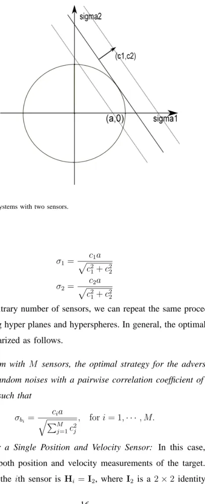
The above problem can be solved by using standard constrained optimization techniques [18] based on gradient and Hessian, which are rather involved. Here we solve the problem using a much simpler geometric solution, which has been shown to give the same solution as that by the standard optimization techniques. We start with the simplest case with two sensors, in which we need to solve the following optimization problem.
max c1σb1 +c2σb2 (66) s.t. σ2 b1 +σ 2 b2 =a 2
We can get the optimal solution by analyzing the problem geometrically with the norm vector
(c1, c2)T of the objective function as shown in Fig. 1. The constraint of the problem is represented
by the circle with a radius ofa. We move the linel1with the slope−
c1
c2
to get the largest intercept between l1 and σ2 axis under the constraint that there is an intersection between the circle and
Fig. 1. Geometric solution for systems with two sensors. circle, which is σ1 = c1a p c2 1 +c 2 2 σ2 = c2a p c2 1 +c 2 2 (67)
For a system with arbitrary number of sensors, we can repeat the same procedure to find the optimal solution by using hyper planes and hyperspheres. In general, the optimal attack strategy can be found and summarized as follows.
Theorem 1. For a system with M sensors, the optimal strategy for the adversary is to inject
statistically correlated random noises with a pairwise correlation coefficient of 1. The random bias power is allocated such that
σbi = cia q PM j=1c 2 j , fori= 1,· · ·, M. (68)
2) Attack Strategy for a Single Position and Velocity Sensor: In this case, let us assume
that the sensors collect both position and velocity measurements of the target. Therefore, the measurement matrix for the ith sensor is Hi =I2, where I2 is a 2×2 identity matrix. At the
ith sensor, the adversary injects the bias noise vector bki to the sensor measurement zki, where bki = [bpi bvi]
T consists of biases in position and velocity measurements. Let us assume that the
system bias vector bk = [bT
k1,· · · ,bTkM]T is zero-mean and has a 2M ×2M covariance matrix ΣK. Further, the (i, j)th 2×2 submatrix for ΣK is defined as
ΣK(i, j) = ρbpi,bpjσbpiσbpj ρbp i,bv jσbp iσbv j ρbv i,bpjσbv iσbpj ρbv i,bv jσbv iσbvj (69)
for 1 ≤ i, j ≤ M. σbp i and σbv i are the position and velocity bias noise standard deviations
at the ith sensor respectively. The ρs are defined as the proper correlation coefficients between components of the bias vector, and ρbp i,bpi = ρbv i,bv i = 1, for 1 ≤ i ≤ M. Since the position
biasbp and velocity bias bv have different units, we need an appropriate constraint for bias noise
power. Here we assume that the total noise power is defined as
M X i=1 σ2 bpi +T 2 σ2 bvi (70)
Note that this is a meaningful power definition, since the two terms in the above equation has the same unit. Recall that according to the target tracking system plant equation and ignoring the system process noise, we haveξk+1 =ξk+Tξ˙k. Therefore, the power defined in (70) can be
interpreted as the summation of the extra mean squared errors for the position estimate caused by independent bias injections. We can see that the best attack strategy derived under a constraint on power defined in (70) can be easily adjusted and extended for other power definitions, as long as in the new definition, the second term is proportional to T2
σ2
bvi.
As we can use the equivalent sensor to represent the multiple sensors, we focus on the single-sensor case first. If we are interested in the case of N = 0, maximizing the trace of AK
is equivalent to maximize the WKΣKWKT. We assume that the adversary knows the system
models and the prior information P0|0 at time zero, so that he/she can calculate the offline
Kalman filter gain matrix Wk recursively. Therefore, the best strategy the adversary can adopt
to attack the system is the solution to the following optimization problem:
max ΣK Tr WKΣKWTK s.t. σ2 bp+T 2 σ2 bv =a 2 −1≤ρbp,bv ≤1 σbp, σbv >0 (71)
where ΣK = σ2 bp ρbp,bvσbpσbv ρbp,bvσbpσbv σ 2 bv (72) and WK = w11 w12 w21 w22 (73)
It is easy to show that
Tr WKΣKWKT = Tr WTKWKΣK = (w2 11+w 2 21)σ 2 bp + (w 2 12+w 2 22)σ 2 bv + 2(w11w12+w21w22)ρbp,bvσbpσbv (74)
According to the sign of (w11w12+w21w22), we can set the value of the ρbp,bv to maximize
the objective function. For example, if (w11w12+w21w22) is positive, we set ρbp,bv = 1 and the
optimization problem becomes
max(w11σbp+w12σbv) 2 + (w21σbp +w22σbv) 2 s.t. σ2 bp +T 2 σ2 bv =a 2 (75) σbp, σbv ≥0
We have solved the optimization problem in (75), and summarize the results in the following theorem.
Theorem 2. For a system with one sensor observing position and velocity of the target, the optimal strategy for the adversary is to inject random noise that has dependent position and velocity components. If w11w12+w21w22>0, the correlation coefficient ρbp,bv should be set as
1, and the random bias power is allocated such that σbp =asin(θ ∗) (76) σbv = a T cos(θ ∗) θ∗ = π 4 − φ 2 φ= arctan β2−β1T2 2T(α1+α2) w2 11+w 2 21=β1 w2 12+w 2 22=β2 w11w12 =α1 w21w22 =α2
Whenw11w12+w21w22 <0, we should setρbp,bv =−1and setα1 =−w11w12andα2 =−w21w22.
The rest of the equations in formula (76) remain the same. Proof Sketches: Let us first denote
w2 11+w 2 21=β1 w2 12+w 2 22=β2 w11w12 =α1 w21w22 =α2 (77)
The constraint in (71) can be written as σ2 bp T2 +σ 2 bv = a2 T2 =a 2 1 (78)
Now we set σbp = a1T sin(θ) and σbv = a1cos(θ). Plugging σbp and σbv into the objective
function, we have the following equivalent optimization problem
max θ a 2 1 β1T12+β2 2 +Asin(2θ+φ) s.t. 0≤θ≤ π 2 (79)
where A = r 1 4(β2 −β1T 2)2+T2(α 1+α2)2 (80) tan(φ) = β2−β1T 2 2T(α1+α2) (81)
Clearly, the optimal solution is
θ∗ = π
4 −
φ
2 (82)
3) Attack Strategy for Multiple Position and Velocity Sensors: In this case, let us consider the
case of M = 2, where the measurement matrix is H = [I2 I2]T. The measurement covariance
matrix for the ith sensor is assumed to be
Ri = σ2 pi 0 0 σ2 vi (83)
Now, according to (55), we have
Re = [R−11+R −1 2 ] −1 = σ−2 p1 +σ− 2 p2 −1 0 0 σ−2 v1 +σ− 2 v2 −1 (84) According to (54), we define Ci =ReHTi R− 1 i = σ−2 pi σ−2 p1+σ −2 p2 0 0 σ− 2 vi σ−2 v1+σ −2 v2 (85)
as the weighting matrix for the ith sensor’s observation zi. Further, we define
cpi =Ci(1,1)
cvi =Ci(2,2)
(86)
both of which are positive numbers. The equivalent noise injection is therefore
beK =
2
X
i=1
CibKi (87)
So the covariance matrix of the equivalent bias vector is
ΣeK = 2 X i=1 2 X i=j CiΣK(i, j)CTj (88)
where ΣK(i, j) has been defined in (69). It can be shown that ΣeK = s1 s2 s2 s3 (89) where s1 =c 2 p1σ 2 bp1 +c 2 p2σ 2 bp2 + 2ρbp1,bp2cp1cp2σbp1σbp2 s3 =c 2 v1σ 2 bv1 +c 2 v2σ 2 bv2 + 2ρbv1,bv2cv1cv2σbv1σbv2 (90) s2 =cp1cv1ρbp1,bv1σbp1σbv1 +cp1cv2ρbp1,bv2σbp1σbv2 +cp2cv1ρbp2,bv1σbp2σbv1 +cp2cv2ρbp2,bv2σbp2σbv2 (91)
The optimization problem can be written as follows.
max ΣeK Tr WeKΣeKWeKT (92) s.t. σ2 bp1 +σ 2 bp2 +T 2 σ2 bv1 +T 2 σ2 bv2 =a 2 , −1≤ρpi,vj ≤1, −1≤ρvi,vj ≤1, −1≤ρpi,pj ≤1, σpi, σvi ≥0, ∀i, j ∈ {1,2} where WeK = w11 w12 w21 w22 (93)
is the Kalman filter gain calculated using the equivalent measurement covariance matrix Re and
equivalent measurement matrix He. It is easy to show that
Tr WKΣKWTK = Tr WTKWKΣK (94) = (w2 11+w 2 21) 2 s1+ (w 2 12+w 2 22) 2 s3 +2(w11w12+w21w22)s2
Clearly, all theρs that appear ins1 ands3 should be set as 1 to maximize the objective function.
w11w12+w21w22>0, all theρs that appear in s2 should be set to 1; otherwise, they should be
set as −1. Let us first suppose that w11w12+w21w22>0 is true, then we have
Tr WKΣKWTK = (w2 11+w 2 21) 2 (cp1σp1 +cp2σp2)2 + (w2 12+w 2 22) 2 (cv1σv1 +cv2σv2)2 + 2(w11w12+w21w22)(cp1cv1σp1σv1 +cp1cv2σp1σv2 +cp2cv1σp2σv1 +cp2cv2σp2σv2) (95)
So far, we have converted the objective function in (92), which involves 10 variables to one that involves only 4 variables. Considering that the power constraint reduces one degree of freedom, we only need to solve an optimization problem in a 3-dimensional space.
4) Strategy for a Single Sensor with Multiple Time Attacks: Based on Proposition 2, we get
the extra mean squared error matrix,
AK+N = N
X
m=0
DmΣK+N−mDTm
Supposing that the adversary attacks the system continuously from time K to K + N, the weighted extra mean squared error matrices at different time are as shown below,
A′K+0 =α0(D0ΣKDT0)
A′K+1 =α1(D0ΣK+1DT0 +D1ΣKDT1) (96)
...
A′K+N =αN(D0ΣK+NDT0 +...+DNΣKDTN)
where αi, i∈ N is the weight of extra mean squared error matrix at time i, and PNi=0αi = 1.
The objective function in the multi-time attack problem is the trace of weighted sum of the extra mean squared error matrices at different time:
Tr N X i=0 αiAK+i ! = Tr N X i=0 A′K+i ! (97)
Maximizing the term above is equivalent to maximize the trace of the weighted sum of the mean squared error matrices of the state estimates over time, because once the system reaches its steady state, PK+i|K+i will be a constant, and the weighted sum ofPK+i|K+i will remain the
same. First we study the case with position sensors only, where all the terms in (96) are scalars. Using lower case d, σp to denote D,Σ, we can formulate the optimization problem below,
max N X i=0 αiAK+i = N X i=0 A′K+i (98) =σ2 pK+0(α0d 2 0+α1d 2 1+...+αNd 2 N) +σ2 pK+1(α1d 2 0+α2d 2 1+...+αNd 2 N−1) +σ2 pK+2(α2d 2 0+α3d 2 1+...+αNd2N−2) +... +σ2 pK+N(αNd 2 0) s.t. K+N X i=K σ2 pi ≤a 2 N X i=0 αi = 1
The adversary can allocate the power based on the coefficient of the variance variables at different time. For example, if the weights α′
is are all the same, the best strategy is to allocate all the
power to the sensor at the first beginning (at time K) because the coefficient for σ2
pK+0 is the
largest.
can be characterized as follows, max Tr " N X m=0 αiAK+i # = Tr " N X m=0 A′K+i # (99) = Tr ΣK+0(α0DT0D0+...+αNDTNDN) +Tr ΣK+1(α1DT0D0+...+αNDTN−1DN−1) +Tr ΣK+2(α2DT0D0+...+αNDTN−2DN−2) +... +Tr ΣK+N(αNDT0D0) s.t. K+N X i=K σ2 pi +T 2 σ2 vi ≤a 2 N X i=0 αi = 1
Since Σi and DTjDj are positive semidefinite matrices, Tr
Σi(DTjDj)
≥ 0. Trace is a mono-tonically increasing function of the positive semidefinite matrix, that is to say, if A and B are both positive semidefinite matrices, and A>B, then T r(A)> T r(B). So the best strategy for the adversary to attack the system is to allocate all the power to Σi with the largest positive
semidefinite matrix of PN
i=sαiDTi−sDi−s. If the adversary’s goal is to maximize the average
effect of the false information, the best strategy is to put all the power at time K.
B. Attack Strategy Analysis from Determinant Perspective
1) Attack Strategy for Multiple Position Sensors: We are also interested in the effect of
bias information on the Kalman filter’s mean squared estimation error from the determinant perspective. By using the equivalent measurement approach as in Section VII-A1, we have
|PK|K+AK|=|PK|K+ ΣeKD0DT0| =|PK|K||I+ ΣeKD0P− 1 K|KD T 0| (100)
where D0 can be obtained using (42) and ΣeK is defined in (63). As PK|K is constant and
positive definite, D0P− 1
K|KDT0 is positive semidefinite meaning that all the eigenvalues of the
D0P− 1
eigenvectors of D0P− 1
K|KDT0. Then through eigendecomposition, (100) can be written concisely
as,
|PK|K||CIC−1+ ΣeKCΛC−1| =|PK|K||I+ ΣeKΛ|
(101)
where Λ is a diagonal matrix whose diagonal elements are the eigenvalues of the D0P− 1
K|KD
T
0.
So we just need to maximize ΣeK in order to maximize the determinant of PK|K+AK. This
is equivalent to maximizing the trace of PK|K+AK as discussed in Section VII-A1.
2) Attack Strategy for a Single Position and Velocity Sensor: We assume that the adversary
knows the system model and the prior informationP0|0 at time zero, so that he/she can calculate
the offline Kalman filter gain matrix Wk recursively. The best attack strategy is the solution to the following optimization problem.
max ΣK PK|K+WKΣKWTK s.t. σ2 bp +T 2 σ2 bv =a 2 (102) −1≤ ρbp,bv ≤1 σbp, σbv >0 where WKΣKWTK =AK, and ΣK = σ2 bp ρbp,bvσbpσbv ρbp,bvσbpσbv σ 2 bv (103)
Using the properties of the determinant, we get the formula as follows.
|PK|K+WKΣKWTK| =|PK|K||In+ΣKWKTP−
1
K|KWK| (104)
Since PK|K is independent of ΣK, the optimization problem can be further written as:
max ΣK In+ΣKW T KP− 1 K|KWK s.t. σ2 bp+T 2 σ2 bv =a 2 (105) −1≤ρbp,bv ≤1 σbp, σbv >0
By defining WTKP−K|K1 WK = m1 m2 m2 m3 (106)
and after simplifying (105), the objective function becomes
In+ΣKW T KP− 1 K|KWK = 1 + (1−ρ2 bp,bv)σ 2 bpσ 2 bv(m1m3−m 2 2) (107) +σ2 bpm1+σ 2 bvm3+ 2ρbp,bvσbpσbvm2
The solution to the optimization problem will be the best strategy to attack the system. In order to get closed-form solutions, we denote ΣK =RTR where ΣK is invertible, and
In+ΣKW T KP− 1 K|KWK = In+R TRWT KP− 1 K|KWK (108) = In+RW T KP− 1 K|KWKRT
To facilitate the derivations, we introduce two lemmas from [19], which are provided below.
Lemma 1. Suppose A and B are n×n positive semidefinite matrices with eigendecomposition
A=DAΣADTA and B =DBΣBDTB, the eigenvalues ofA and B satisfy that α1 ≥α ≥ · · ·αn
and β1 ≥β ≥ · · ·βn, then
Πni=1(αi+βi)≤det(A+B)≤Π
n
i=1(αi+βn+1−i) (109)
where the upper bound is achieved if and only if DA=DBP, and the lower bound is achieved
if and only if DA =DB, where P is defined below,
P= 0 0 · · · 1 0 · · · 1 0 .. . ... ... ... 1 0 · · · 0 (110)
The optimal solution achieving the upper bound is the best attack strategy with the most effect on the Kalman filter system, and that achieving the lower bound is the strategy with the least effect on the Kalman filter system.
Lemma 2. Given ann×nmatrixV1 and ann×npositive semidefinite matrixQ1 withV1Q1VT1 being a diagonal matrix with its diagonal elements in increasing order, it is always possible to find another n×n matrix V¯1 such that V¯1Q1V¯T1 =βV1Q1V1T with T r(V1V1T) =T r( ¯V1V¯T1) where β ≥ 1. V¯1 can be written as ΣQDT1, where D1 is the unitary matrix whose columns are the eigenvectors corresponding to the eigenvalues of Q1 in increasing order, and ΣQ is a
diagonal matrix.
By combining the two lemmas together, we can get the final optimal solution to the optimiza-tion problem above. It is obvious that In and RWTKP−
1
K|KWKRT are both positive semidefinite
matrices. The eigendecomposition of the two items above can be written as follows,
In =DIΣ1DTI
RWTKP−K|K1 WKRT =D2Σ2DT2 (111)
with identity matrix Σ1 and Σ2 =diag([σ2,1,· · · , σ2,n]). Based on Lemma 1, we have
In+RW T KP− 1 K|KWKR T ≤Π n i=1(σ1,i+ 1) (112) where D2P=D1, and |In+RWTKP− 1 K|KWKR T| =|DT1||In+RW T KP− 1 K|KWKR T||D 1| (113) =|In+DT1RW T KP− 1 K|KWKR TD 1|
Set R1 =DT1R and Σ3 =PΣ2PT with the eigenvalues in increasing order and we know that
T r(RRT) =T r(R1RT1). So the optimization problem can be written as below,
max |In+R1WTKP− 1 K|KWKR T 1| s.t. T r(R1RT1)≤a 2 (114) R1WKTP− 1 K|KWKR T 1 =Σ3
Let us set WTKP−K|K1 WK = ˜Q. Based on Lemma 2, R1QR˜ T1 = Σ3, we can surely find a
matrix R¯ such that R¯1Q ¯˜RT1 =βR1QR˜ T1, for β ≥1. Note that the determinant is a monotonic
increasing function of the positive semidefinite matrix. So
So the optimal solution R¯ should be in the form of V¯. The eigendecompostion of Q˜ is as follows,
˜
Q=VQΣQVQT (116)
where ΣQ =diag([σq,1, σq,2,· · · , σq,n]) with its diagonal elements in increasing order. VQ is a
unitary matrix whose column vectors correspond to the eigenvalues of Q˜. The problem can be written as max σ2 b,i n X i=1 log(σ2 b,iσq,i+ 1) (117) s.t. n X i=1 (σ2 b,i)≤a 2
The objective function above is a concave and increasing function. The optimal solution is achieved through Lagrangian multipliers yielding the water-filling strategy,
σ2 b,i = 1 λ − 1 σq,i + (118)
where the value of λ can be obtained by solving
n X i=1 1 λ − 1 σq,i + =a2 (119) The solution is Ropt=D1[Σ 1/2 b ]TVTQ (120)
Finally, the optimal solution of (105) is,
ΣK =VQΣbVTQ (121)
Theorem 3. For a system with one sensor that provides position and velocity measurements, the optimal strategy for the adversary to attack the system in order to maximize the determinant of mean squared error matrix is
ΣK =VQΣbVTQ (122) where Σb =diag([σb,21, σ 2 b,2,· · · , σ 2 b,n]) , σ 2 b,i = 1 λ − 1 σq,i + and Pn i=1 1 λ − 1 σq,i + =a2 , VQ is
a unitary matrix whose column vectors corresponds to the eigenvalues σq,i’s of WTKP−
1
K|KWK,
3) Attack Strategy for Multiple Position and Velocity Sensors: For a system with multiple
sensors, the best strategy to allocate the bias noise power and set the correlation coefficients among the bias noises at different sensors is also investigated. Let us denote the number of sensors as M, and the measurement matrix as H= [I2,· · · ,I2]T. The measurement covariance
matrix for the ith sensor is assumed to be
Ri = σ2 pi 0 0 σ2 vi (123)
Now, according to (53), we have
Re = M X i=1 R−1 i !−1 = PM i=1σ− 2 pi −1 0 0 PM i=1σ −2 vi −1 (124) According to (51), we define Ci =ReR−1 i = σ−2 pi PM j=1σ− 2 pj 0 0 σ− 2 vi PM j=1σ− 2 vj (125)
as the weighting matrix for the ith sensor’s observation zi. The equivalent injected bias noise is therefore
beK = M
X
i=1
CibKi (126)
and the covariance matrix of the equivalent bias vector is
ΣeK = M X i=1 M X j=1 CiE bibTj CTj (127)
Now the optimization problem can be formulated as follows. max ΣeK PK|K+WeKΣeKWTeK (128) s.t. N X i=1 σ2 bpi +T 2 N X j=1 σ2 bvi =a 2 , −1≤ρbpi,bvj ≤1, −1≤ρbvi,bvj ≤1, −1≤ρbpi,bpj ≤1, σbpi, σbvi ≥0, ∀i, j ∈ {1, M}
whereWeK is the Kalman filter gain calculated using HeandRe. The optimal solution of (128)
VIII. NUMERICAL RESULTS
Numerical results are presented in this chapter to demonstrate the effectiveness of the derived attack strategies.
A. Systems with Position Sensors
The parameters used in the target tracking example are provided below. The system sampling interval is T = 1. The adversary injects bias information to two sensors with σ2
w1 = 3 and
σ2
w2 = 4, respectively. The variance of the system process noise is σ
2
v = 0.25. The biases bis are
zero-mean Gaussian random variables with variancesσ2
bis. For the power constraint we discussed
earlier, we set the sum of σ2
bi to be 3000.
The effect of the bias injection on the Kalman filter is measured by the normalized MSE. More specifically, we use the sum of the normalized MSE over Nm Monte-Carlo runs
qk = Nm X j=1 h ˆ x′jk|k−xjkiT Pk|k−1hxˆ′jk|k−xjki (129) where at timek,Pk|kis the nominal state covariance matrix calculated by the Kalman filter,xˆ′jk|k
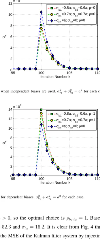
is the state estimate, andxjkis the true state, during the jth Monte-Carlo run. First, if the random biases injected to different sensors are independent, we should allocate all the bias power to the sensor with the smallest measurement noise variance. This is clearly true as demonstrated in Fig. 2, where allocating all the power to sensor 1 causes the maximum mean squared estimation error. In Fig. 3, three dependent-noise attack strategies are compared, including the optimal one according to (67), allocating the power equally among the sensors, and allocating all the power to the sensor with the smallest measurement error variance. It is clear that the optimal solution has the largest impact on the estimation performance, and it outperforms the best independent-noise attack strategy significantly.
B. Systems with Position and Velocity Sensors
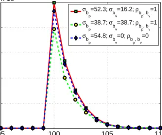
We now consider the case where the adversary attacks the Kalman filtering system with a vector sensor observation containing both position and velocity measurements. We first consider a single-sensor system, and the sensor has a position measurement variance of 3 and a velocity measurement variance of 4. We set the sum of σ2
bp1 and T
2
σ2
95 100 105 110 0 2 4 6 8 10 12x 10 4 Iteration Number k q k σb1=0.8a; σ b2=0.6a; ρ=0 σb1=0.7a; σb2=0.7a; ρ=0 σb1=a; σb2=0; ρ=0
Fig. 2. The normalized MSE when independent biases are used.σb21+σ 2 b2 =a
2
for each case.
95 100 105 110 0 2 4 6 8 10 12 14x 10 4 Iteration Number k q k σb1=0.8a; σb2=0.6a; ρ=1 σb1=0.7a; σb2=0.7a; ρ=1 σb1=a; σ b2=0; ρ=0
Fig. 3. The normalized MSE for dependent biases.σ2 b1+σ
2 b2 =a
2
for each case.
case, w11w12+w21w22 >0, so the optimal choice is ρbp,bv = 1. Based on Theorem 2, the best
strategy is to set σbp = 52.3 and σbv = 16.2. It is clear from Fig. 4 that the strategy provided in
Theorem 2 maximizes the MSE of the Kalman filter system by injecting vector bias information.
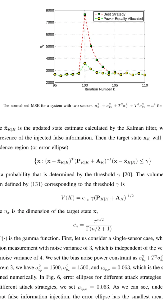
Next we consider a system with two sensors. The first sensor is the same as the one described above, and the second one is with position measurement variance 4 and velocity measurement
95 100 105 110 0 1 2 3 4 5x 10 5 Iteration Number k q k σb p =52.3; σ b v =16.2; ρ b p, bv =1 σb p =38.7; σ b v =38.7; ρ b p, bv =1 σb p =54.8; σ b v =0; ρ b p, bv =0
Fig. 4. The normalized MSE for a system with a single sensor.σ2p1+T 2
σv21=a 2
for each case.
variance 5. In this particular case, again we have w11w12+w21w22 >0, so all the ρs in s1, s2,
and s3 should be set as 1. We first use a systematic grid search to find an approximate globally
optimal solution and then we use the FMINCON function in Matlab, a local search algorithm, to refine this approximate globally optimal solution. The optimal solution we have obtained is σ2 bp1 = 1826, σ 2 bp2 = 1023, σ 2 bv1 = 81, σ 2
bv2 = 68. For comparison purpose, we also implement
an attack strategy that allocate power equally among the observation components and among the two sensors, which is σ2
bp1 = σ 2 bp2 =σ 2 bv1 = σ 2
bv2 = 750. The simulation result is shown in
Fig. 5. As we can see, the optimal attack strategy has a much greater impact than the one that allocates power equally. Based on the optimal solution, we can find that allocating more power to the measurement with lower variance will have a greater effect on the Kalman filter system.
C. Determinant Case
Numerical results are presented in this section to illustrate the effectiveness of the proposed attack strategies. Assuming that the injected bias noisebkis zero-mean and Gaussian distributed,
we can show that the posterior probability density function (PDF) of the target state conditioned on the past observations and the current corrupted observation is
95 100 105 110 2000 3000 4000 5000 6000 7000 8000 Iteration Number k q k Best Strategy
Power Equally Allocated
Fig. 5. The normalized MSE for a system with two sensors.σ2p1+σ 2 p2+T 2 σv21+T 2 σv22=a 2
for each case.
where xˆK|K is the updated state estimate calculated by the Kalman filter, which is unaware of the presence of the injected false information. Then the target state xK will be in the following
confidence region (or error ellipse)
x: (x−ˆxK|K)T(PK|K+AK)−1(x−xˆK|K)≤γ (131)
with a probability that is determined by the threshold γ [20]. The volume of the confidence region defined by (131) corresponding to the threshold γ is
V(K) =cnx|γ(PK|K +AK)|
1/2
(132)
where nx is the dimension of the target state x,
cn =
πn/2
Γ(n/2 + 1) (133)
andΓ(·)is the gamma function. First, let us consider a single-sensor case, where the sensor has a position measurement with noise variance of3, which is independent of the velocity measurement with noise variance of4. We set the bias noise power constraint asσ2
bp+T 2 σ2 bv = 3000. Based on Theorem 3, we haveσ2 bp = 1500, σ 2
bv = 1500, andρbp,v = 0.063, which is the same as the solution
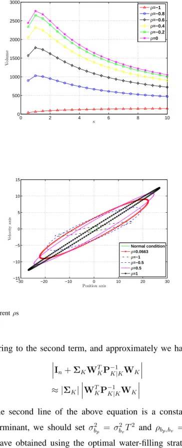
obtained numerically. In Fig. 6, error ellipses for different attack strategies are plotted. For all the different attack strategies, we set ρbp,v = 0.063. As we can see, under normal condition
−40 −30 −20 −10 0 10 20 30 40 −15 −10 −5 0 5 10 15 Position axis V el o ci ty a x is Normal condition σ2 b p =1500,σ2 b v =1500 σ2 b p =0,σ2 b v =3000 σ2 b p =1000,σ2 b v =2000 σ2 b p =3000,σ2 b v =0
Fig. 6. Error ellipses for different power allocation strategies
attack strategy leads to an error ellipse with the largest area. In Figs. 7 and 8, the volume (area) of the error ellipse is provided as a function of ρbp,v and the ratio κ =
σbp
σbvT. We can see that
when the κ = σbp
σbvT = 1, the area of the ellipse is maximized. Also from Figs. 7 and 8, it is
clear that the area of ellipse increases as the absolute value of ρ decreases. In Fig. 9, the trend of the error ellipses as the ρ changes from −1 to +1 is illustrated.
0 2 4 6 8 10 0 500 1000 1500 2000 2500 3000 κ V o lu m e ρ=0 ρ=0.2 ρ=0.4 ρ=0.6 ρ=0.8 ρ=1
Fig. 7. Error ellipses volume
In this particular case, since σ2
bp +T
2
σ2
bv = 3000, ΣK is large and in (102) the second term
(WKΣKWT
0 2 4 6 8 10 0 500 1000 1500 2000 2500 3000 κ V o lu m e ρ=−1 ρ=−0.8 ρ=−0.6 ρ=−0.4 ρ=−0.2 ρ=0
Fig. 8. Error ellipses volume
−30 −20 −10 0 10 20 30 −15 −10 −5 0 5 10 15 Position axis V el o ci ty a x is Normal condition ρ=0.0663 ρ=−1 ρ=−0.5 ρ=0.5 ρ=1
Fig. 9. Error ellipses for differentρs
relatively small comparing to the second term, and approximately we have
In+ΣKW T KP− 1 K|KWK ≈ |ΣK| W T KP− 1 K|KWK (134)
The second term in the second line of the above equation is a constant. Hence, in order to get the maximum determinant, we should set σ2
bp = σ
2
bvT
2
and ρbp,bv = 0. This is almost the
same solution as we have obtained using the optimal water-filling strategy. Next we consider a system with two sensors. The first sensor is the same as the one described above, and the
−8 −6 −4 −2 0 2 4 6 8 −4 −3 −2 −1 0 1 2 3 4 Position axis V el o ci ty a x is Normal condition Optimal attack Attack strategy I Attack strategy II Attack strategy III
Fig. 10. Error ellipses for different power allocation strategies
second one is with position measurement variance 4 and velocity measurement variance 5. To solve the optimization problem formulated in (128), we first use a systematic grid search to find an approximate globally optimal solution and then we use the FMINCON function in Matlab, a local search algorithm, to refine this approximate globally optimal solution. The optimal solution we have obtained is σ2
bp1 = 1100, σ 2 bp2 = 600, σ 2 bv1 = 750, σ 2 bv2 = 550, ρbp1,p2 = 0.99, ρbp1,v1 = −0.83, ρbp1,v2 = 0.75, ρbv1,p2 = 0.89, ρbp2,v2 = −0.23, ρbv1,v2 = 0.95.
For comparison purpose, we introduce three sub-optimal attack strategies: Strategy I with all the ρs being 0s, and σ2
bp1 = 1100, σ 2 bp2 = 600, σ 2 bv1 = 750, σ 2
bv2 = 550; Strategy II with all the
ρs being 1s, and σ2 bp1 = 1100, σ 2 bp2 = 600, σ 2 bv1 = 750, σ 2
bv2 = 550; and Strategy III with the ρs
being the same as those for the optimal strategy, and σ2
bp1 = σ 2 bp2 = σ 2 bv1 = σ 2 bv2 = 750. The
numerical results are shown in Fig. 10. As we can see, the optimal attack strategy has a greater impact than those sub-optimal attack strategies, resulting in the largest error ellipse.
IX. CONCLUSION
In this thesis, the impact of false information injection on the Kalman filter’s state estimation was studied. We derived the EMSE due to the injected random biases for a Kalman filter in a linear dynamic system. This allows us to find how to allocate the bias power among multiple sensors in order to maximize the effect of the false information on the Kalman filter from two perspectives: trace and determinant of the MSE matrix. By using the equivalent sensor to denote the multiple sensors in the Kalman filter system, the analysis of optimization problem is simplified a lot. A concrete example of multi-sensor target tracking system has been provided. In this example, we investigated both the case where the sensors provide position measurements and the case where they collect both position and velocity measurements. For the case where the sensors provide only position measurements, we have found that the dependent false information will incur more Kalman filter system state estimation error than the independent one does. From the trace and determinant perspectives, many closed-form results have been provided for the optimal attack strategies. In the future, we will use game theory and hypothesis testing techniques to characterize the model in order to have a better understanding of the false information attacks and Kalman filter’s defense against such attacks.
REFERENCES
[1] Y. Liu, M.K. Reiter, and P. Ning, “False data injection attacks agianst state estimation in electric power grids,” in Proc. the 16th ACM Conference on Computer and Communications Security, Chicago, IL, November 2009.
[2] L. Jia, R.J. Thomas, and L. Tong, “Malicious data attack on real-time electricity market,” in Proc. International Conference on Acoustics, Speech, and Signal Processing, Prague, Czech Republic, May 2011, pp. 5952–5955.
[3] O. Kosut, L. Jia, R. J. Thomas, and L. Tong, “Malicious Data Attack on Smart Grid State Estimation: Attack Strategies and Countermeasures,” in Proc. First IEEE International Conference on Smart Grid Communications (SmartGridComm), Gaithersburg, MD, Oct. 2010, pp. 220–225.
[4] L. Jia, R. J. Thomas, and L. Tong, “On the nonlinearity effects on malicious data attack on power system,” in Proc. Power and Energy Society General Meeting, San Diego, CA, July 2012, pp. 1–8.
[5] M. A. Rahman and H. Mohsenian-Rad, “False data injection attacks with incomplete information against smart power grids,” in Proc. Global Communications Conference, San Diego, CA, Dec. 2012, pp. 3153–3158.
[6] J. Kim, L. Tong, and R. J. Thomas, “Data framing attack on state estimation,” IEEE Trans. on Aerospace and Electronic Systems, vol. 49, no. 3, pp. 1637–1653, July 2013.
[7] J.Kim, L. Tong, and R.J. Thomas, “Data framing attack on state estimation with unknown network parameters,” in Proc. of the Asilomar Conference on Signals, Systems and Computers, Pacific Grove, CA, Nov 2013, pp. 1388 – 1392. [8] J.Kim, L. Tong, and R.J. Thomas, “Subspace methods for data attack on state estimation: A data driven approach,” IEEE
Trans. on Signal Processing, vol. 63, no. 5, pp. 1102 – 1114, Dec 2014.
[9] X. Song, P. Willett, S. Zhou, and P. B. Luh, “The mimo radar and jammer games,” IEEE Trans. on Signal Processing, vol. 60, no. 2, pp. 687–699, February 2012.
[10] C. Yang, L. Kaplan, and E. Blasch, “Performance measures of covariance and information matrices in resource management for target state estimation,” IEEE Trans. on Aerospace and Electronic Systems, vol. 48, no. 3, pp. 2594–2612, July 2012. [11] C. Yang, L. Kaplan, E. Blasch, and M. Bakich, “Optimal placement of heterogeneous sensors for targets with gaussian
priors,” IEEE Trans. on Aerospace and Electronic Systems, vol. 49, no. 3, pp. 1637–1653, July 2013.
[12] E. Masazade, R. Niu, P.K. Varshney, and M. Keskinoz, “Energy aware iterative source localization for wireless sensor networks,” IEEE Trans. on Signal Processing, vol. 58, no. 9, pp. 4824–4835, September 2010.
[13] E. Masazade, R. Niu, and P.K. Varshney, “Dynamic bit allocation for object tracking in wireless sensor networks,” IEEE Trans. on Signal Processing, vol. 60, no. 10, pp. 5048–5063, October 2012.
[14] X. Lin and Y. Bar-Shalom, “Multisensor target tracking performance with bias compensation,” IEEE Trans. Aerosp. Electron. Syst., vol. 42, no. 3, pp. 1139–1149, July 2006.
[15] R. Niu and L. Huie, “System State Estimation in the Presence of False Information Injection,” in Statistical Signal Processing Workshop (SSP), Ann Arbor, MI, Aug. 2012, pp. 385–388.
[16] Y. Bar-Shalom, X.R. Li, and T. Kirubarajan, Estimation with Applications to Tracking and Navigation, Wiley, New York, 2001.
[17] R. Niu, “Dynamic System State Estimation in the Presence of Continuous False Information Injection,” Tech. Rep., Extension Grant from Visiting Faculty Research Program, Air Force Research Laboratory Information Directorate, March 2012.
[18] S. Boyd and L. Vandenberghe, Convex Optimization, Cambridge Univ. Press, Cambridge, U.K., 2004.
[19] B. Tang, J. Tang, and Y. Peng, “Mimo radar waveform design in colored noise based on information theory,” IEEE Trans. on Signal Processing, vol. 58, no. 9, pp. 4684 – 4697, September 2010.
[20] Y. Bar-Shalom, P.K. Willett, and X. Tian, Tracking and Data Fusion: A Handbook of Algorithms, YBS Publishing, Storrs, CT, 2011.