Towards quantum machine learning with tensor networks

(1)

Recent Work

Title

Towards quantum machine learning with tensor networks

Permalink

https://escholarship.org/uc/item/8c00q6n5

Journal

Quantum Science and Technology, 4(2)

ISSN

2058-9565

Authors

Huggins, William

Patil, Piyush

Mitchell, Bradley

et al.

Publication Date

2019-04-01

DOI

10.1088/2058-9565/aaea94

Peer reviewed

eScholarship.org

Powered by the California Digital Library

(2)

William Huggins,1 _{Piyush Patil,}1 _{Bradley Mitchell,}1 _{K. Birgitta Whaley,}1 _{and E. Miles Stoudenmire}2 1

University of California Berkeley, Berkeley, CA 94720 USA

2_{Center for Computational Quantum Physics, Flatiron Institute, 162 5th Avenue, New York, NY 10010, USA}

(Dated: August 1, 2018)

Machine learning is a promising application of quantum computing, but challenges remain as near-term devices will have a limited number of physical qubits and high error rates. Motivated by the usefulness of tensor networks for machine learning in the classical context, we propose quantum computing approaches to both discriminative and generative learning, with circuits based on tree and matrix product state tensor networks that could have benefits for near-term devices. The result is a unified framework where classical and quantum computing can benefit from the same theoretical and algorithmic developments, and the same model can be trained classically then transferred to the quantum setting for additional optimization. Tensor network circuits can also provide qubit-efficient schemes where, depending on the architecture, the number of physical qubits required scales only logarithmically with, or independently of the input or output data sizes. We demonstrate our proposals with numerical experiments, training a discriminative model to perform handwriting recognition using a optimization procedure that could be carried out on quantum hardware, and testing the noise resilience of the trained model.

I. INTRODUCTION

For decades, quantum computing has promised to rev-olutionize certain computational tasks. It now appears that we stand on the eve of the first experimental demon-stration of a quantum advantage [1]. With noisy, inter-mediate scale quantum computers around the corner, it is natural to investigate the most promising applications of quantum computers and to determine how best to har-ness the limited, yet powerful resources they offer.

Machine learning is a very appealing application for quantum computers because the theories of learning and of quantum mechanics both involve statistics at a fun-damental level, and machine learning techniques are in-herently resilient to noise, which may allow realization by near-term quantum computers operating without er-ror correction. But major obstacles include the limited number of qubits in near-term devices and the chal-lenges of working with real data. Real data sets may contain millions of samples, and individual samples are typically vectors with hundreds or thousands of compo-nents. Therefore one would like to find quantum algo-rithms that can perform meaningful tasks for large sets of high-dimensional samples even with a small number of noisy qubits.

The quantum algorithms we propose in this work implement machine learning tasks—both discriminative and generative—using circuits equivalent to tensor net-works [2–4], specifically tree tensor netnet-works [5–8] and matrix product states [2, 9, 10]. Tensor networks have recently been proposed as a promising architecture for machine learning with classical computers [11–13], and provide good results for both discriminative [12–18] and generative learning tasks [19, 20].

The circuits we will study contain many parameters which are not determined at the outset, in contrast to quantum algorithms such as Grover search or Shor factor-ization [21, 22]. Only the circuit geometry is fixed, while

D= 4

<latexit sha1_base64="JFP3kCp4Tz8drI6GelidaLuTbAk=">AAACuHicdVFNSwMxEE3X7/pV9egluAieym4RVEQQ9OBR0arQXWQ2na6hSXZJskpZ+xO86tW/5b8xXXtQWwcCjzfv5U0ySS64sUHwWfNmZufmFxaX6ssrq2vrjY3NW5MVmmGbZSLT9wkYFFxh23Ir8D7XCDIReJf0z0b9uyfUhmfqxg5yjCWkivc4A+uo6/OT/YeGHzSDqugkCMfAJ+O6fNiofUTdjBUSlWUCjOmEQW7jErTlTOCwHhUGc2B9SLHjoAKJJi6rWYd01zFd2su0O8rSiv3pKEEaM5CJU0qwj+Zvb0RO63UK2zuMS67ywqJi30G9QlCb0dHDaZdrZFYMHACmuZuVskfQwKz7nnqk8JllUoLqllEf7bATxmWEyhQaR1nlix9GGlTqHjj8rU40TKgjUUn98GWKurq+NdVAncNv0X+S4Cn9L8kZf7jcTsO/G5wE7VbzqBlc7funZ+PlLpJtskP2SEgOyCm5IJekTRhJySt5I+/esQde6vFvqVcbe7bIr/L0F6Yz3Ac=</latexit><latexit sha1_base64="JFP3kCp4Tz8drI6GelidaLuTbAk=">AAACuHicdVFNSwMxEE3X7/pV9egluAieym4RVEQQ9OBR0arQXWQ2na6hSXZJskpZ+xO86tW/5b8xXXtQWwcCjzfv5U0ySS64sUHwWfNmZufmFxaX6ssrq2vrjY3NW5MVmmGbZSLT9wkYFFxh23Ir8D7XCDIReJf0z0b9uyfUhmfqxg5yjCWkivc4A+uo6/OT/YeGHzSDqugkCMfAJ+O6fNiofUTdjBUSlWUCjOmEQW7jErTlTOCwHhUGc2B9SLHjoAKJJi6rWYd01zFd2su0O8rSiv3pKEEaM5CJU0qwj+Zvb0RO63UK2zuMS67ywqJi30G9QlCb0dHDaZdrZFYMHACmuZuVskfQwKz7nnqk8JllUoLqllEf7bATxmWEyhQaR1nlix9GGlTqHjj8rU40TKgjUUn98GWKurq+NdVAncNv0X+S4Cn9L8kZf7jcTsO/G5wE7VbzqBlc7funZ+PlLpJtskP2SEgOyCm5IJekTRhJySt5I+/esQde6vFvqVcbe7bIr/L0F6Yz3Ac=</latexit><latexit sha1_base64="JFP3kCp4Tz8drI6GelidaLuTbAk=">AAACuHicdVFNSwMxEE3X7/pV9egluAieym4RVEQQ9OBR0arQXWQ2na6hSXZJskpZ+xO86tW/5b8xXXtQWwcCjzfv5U0ySS64sUHwWfNmZufmFxaX6ssrq2vrjY3NW5MVmmGbZSLT9wkYFFxh23Ir8D7XCDIReJf0z0b9uyfUhmfqxg5yjCWkivc4A+uo6/OT/YeGHzSDqugkCMfAJ+O6fNiofUTdjBUSlWUCjOmEQW7jErTlTOCwHhUGc2B9SLHjoAKJJi6rWYd01zFd2su0O8rSiv3pKEEaM5CJU0qwj+Zvb0RO63UK2zuMS67ywqJi30G9QlCb0dHDaZdrZFYMHACmuZuVskfQwKz7nnqk8JllUoLqllEf7bATxmWEyhQaR1nlix9GGlTqHjj8rU40TKgjUUn98GWKurq+NdVAncNv0X+S4Cn9L8kZf7jcTsO/G5wE7VbzqBlc7funZ+PlLpJtskP2SEgOyCm5IJekTRhJySt5I+/esQde6vFvqVcbe7bIr/L0F6Yz3Ac=</latexit>

h

0

|

<latexit sha1_base64="Jt93F4dYNDzyEEPAyamQ54qlMrI=">AAACvHicdVHLSsNAFJ3Gd33r0s1gEFyVpAjqSsGNSwVrhSbIzfS2DpmZhJlJpcR8hFvd+Fv+jdPYhdp6YeBw7jlzX0kuuLFB8NnwFhaXlldW15rrG5tb2zu7e/cmKzTDDstEph8SMCi4wo7lVuBDrhFkIrCbpFeTfHeE2vBM3dlxjrGEoeIDzsA6qhslGsqgetzxg1ZQB50F4RT4ZBo3j7uNj6ifsUKiskyAMb0wyG1cgracCayaUWEwB5bCEHsOKpBo4rLut6JHjunTQabdU5bW7E9HCdKYsUycUoJ9Mn9zE3JerlfYwVlccpUXFhX7LjQoBLUZnQxP+1wjs2LsADDNXa+UPYEGZt2KmpHCZ5ZJCapfRinaqhfGZYTKFBontcoXP4w0qKEbsPqtdmucUUeilvrhyxx1/X17roE6h9+m/1SC0fC/Ss74w+VuGv694CzotFvnreD2xL+8mh53lRyQQ3JMQnJKLsk1uSEdwkhKXskbefcuPPRST35LvcbUs09+hTf6AvII3jM=</latexit><latexit sha1_base64="Jt93F4dYNDzyEEPAyamQ54qlMrI=">AAACvHicdVHLSsNAFJ3Gd33r0s1gEFyVpAjqSsGNSwVrhSbIzfS2DpmZhJlJpcR8hFvd+Fv+jdPYhdp6YeBw7jlzX0kuuLFB8NnwFhaXlldW15rrG5tb2zu7e/cmKzTDDstEph8SMCi4wo7lVuBDrhFkIrCbpFeTfHeE2vBM3dlxjrGEoeIDzsA6qhslGsqgetzxg1ZQB50F4RT4ZBo3j7uNj6ifsUKiskyAMb0wyG1cgracCayaUWEwB5bCEHsOKpBo4rLut6JHjunTQabdU5bW7E9HCdKYsUycUoJ9Mn9zE3JerlfYwVlccpUXFhX7LjQoBLUZnQxP+1wjs2LsADDNXa+UPYEGZt2KmpHCZ5ZJCapfRinaqhfGZYTKFBontcoXP4w0qKEbsPqtdmucUUeilvrhyxx1/X17roE6h9+m/1SC0fC/Ss74w+VuGv694CzotFvnreD2xL+8mh53lRyQQ3JMQnJKLsk1uSEdwkhKXskbefcuPPRST35LvcbUs09+hTf6AvII3jM=</latexit><latexit sha1_base64="Jt93F4dYNDzyEEPAyamQ54qlMrI=">AAACvHicdVHLSsNAFJ3Gd33r0s1gEFyVpAjqSsGNSwVrhSbIzfS2DpmZhJlJpcR8hFvd+Fv+jdPYhdp6YeBw7jlzX0kuuLFB8NnwFhaXlldW15rrG5tb2zu7e/cmKzTDDstEph8SMCi4wo7lVuBDrhFkIrCbpFeTfHeE2vBM3dlxjrGEoeIDzsA6qhslGsqgetzxg1ZQB50F4RT4ZBo3j7uNj6ifsUKiskyAMb0wyG1cgracCayaUWEwB5bCEHsOKpBo4rLut6JHjunTQabdU5bW7E9HCdKYsUycUoJ9Mn9zE3JerlfYwVlccpUXFhX7LjQoBLUZnQxP+1wjs2LsADDNXa+UPYEGZt2KmpHCZ5ZJCapfRinaqhfGZYTKFBontcoXP4w0qKEbsPqtdmucUUeilvrhyxx1/X17roE6h9+m/1SC0fC/Ss74w+VuGv694CzotFvnreD2xL+8mh53lRyQQ3JMQnJKLsk1uSEdwkhKXskbefcuPPRST35LvcbUs09+hTf6AvII3jM=</latexit> h0

|

<latexit sha1_base64="Jt93F4dYNDzyEEPAyamQ54qlMrI=">AAACvHicdVHLSsNAFJ3Gd33r0s1gEFyVpAjqSsGNSwVrhSbIzfS2DpmZhJlJpcR8hFvd+Fv+jdPYhdp6YeBw7jlzX0kuuLFB8NnwFhaXlldW15rrG5tb2zu7e/cmKzTDDstEph8SMCi4wo7lVuBDrhFkIrCbpFeTfHeE2vBM3dlxjrGEoeIDzsA6qhslGsqgetzxg1ZQB50F4RT4ZBo3j7uNj6ifsUKiskyAMb0wyG1cgracCayaUWEwB5bCEHsOKpBo4rLut6JHjunTQabdU5bW7E9HCdKYsUycUoJ9Mn9zE3JerlfYwVlccpUXFhX7LjQoBLUZnQxP+1wjs2LsADDNXa+UPYEGZt2KmpHCZ5ZJCapfRinaqhfGZYTKFBontcoXP4w0qKEbsPqtdmucUUeilvrhyxx1/X17roE6h9+m/1SC0fC/Ss74w+VuGv694CzotFvnreD2xL+8mh53lRyQQ3JMQnJKLsk1uSEdwkhKXskbefcuPPRST35LvcbUs09+hTf6AvII3jM=</latexit><latexit sha1_base64="Jt93F4dYNDzyEEPAyamQ54qlMrI=">AAACvHicdVHLSsNAFJ3Gd33r0s1gEFyVpAjqSsGNSwVrhSbIzfS2DpmZhJlJpcR8hFvd+Fv+jdPYhdp6YeBw7jlzX0kuuLFB8NnwFhaXlldW15rrG5tb2zu7e/cmKzTDDstEph8SMCi4wo7lVuBDrhFkIrCbpFeTfHeE2vBM3dlxjrGEoeIDzsA6qhslGsqgetzxg1ZQB50F4RT4ZBo3j7uNj6ifsUKiskyAMb0wyG1cgracCayaUWEwB5bCEHsOKpBo4rLut6JHjunTQabdU5bW7E9HCdKYsUycUoJ9Mn9zE3JerlfYwVlccpUXFhX7LjQoBLUZnQxP+1wjs2LsADDNXa+UPYEGZt2KmpHCZ5ZJCapfRinaqhfGZYTKFBontcoXP4w0qKEbsPqtdmucUUeilvrhyxx1/X17roE6h9+m/1SC0fC/Ss74w+VuGv694CzotFvnreD2xL+8mh53lRyQQ3JMQnJKLsk1uSEdwkhKXskbefcuPPRST35LvcbUs09+hTf6AvII3jM=</latexit><latexit sha1_base64="Jt93F4dYNDzyEEPAyamQ54qlMrI=">AAACvHicdVHLSsNAFJ3Gd33r0s1gEFyVpAjqSsGNSwVrhSbIzfS2DpmZhJlJpcR8hFvd+Fv+jdPYhdp6YeBw7jlzX0kuuLFB8NnwFhaXlldW15rrG5tb2zu7e/cmKzTDDstEph8SMCi4wo7lVuBDrhFkIrCbpFeTfHeE2vBM3dlxjrGEoeIDzsA6qhslGsqgetzxg1ZQB50F4RT4ZBo3j7uNj6ifsUKiskyAMb0wyG1cgracCayaUWEwB5bCEHsOKpBo4rLut6JHjunTQabdU5bW7E9HCdKYsUycUoJ9Mn9zE3JerlfYwVlccpUXFhX7LjQoBLUZnQxP+1wjs2LsADDNXa+UPYEGZt2KmpHCZ5ZJCapfRinaqhfGZYTKFBontcoXP4w0qKEbsPqtdmucUUeilvrhyxx1/X17roE6h9+m/1SC0fC/Ss74w+VuGv694CzotFvnreD2xL+8mh53lRyQQ3JMQnJKLsk1uSEdwkhKXskbefcuPPRST35LvcbUs09+hTf6AvII3jM=</latexit>

h

0

|

<latexit sha1_base64="Jt93F4dYNDzyEEPAyamQ54qlMrI=">AAACvHicdVHLSsNAFJ3Gd33r0s1gEFyVpAjqSsGNSwVrhSbIzfS2DpmZhJlJpcR8hFvd+Fv+jdPYhdp6YeBw7jlzX0kuuLFB8NnwFhaXlldW15rrG5tb2zu7e/cmKzTDDstEph8SMCi4wo7lVuBDrhFkIrCbpFeTfHeE2vBM3dlxjrGEoeIDzsA6qhslGsqgetzxg1ZQB50F4RT4ZBo3j7uNj6ifsUKiskyAMb0wyG1cgracCayaUWEwB5bCEHsOKpBo4rLut6JHjunTQabdU5bW7E9HCdKYsUycUoJ9Mn9zE3JerlfYwVlccpUXFhX7LjQoBLUZnQxP+1wjs2LsADDNXa+UPYEGZt2KmpHCZ5ZJCapfRinaqhfGZYTKFBontcoXP4w0qKEbsPqtdmucUUeilvrhyxx1/X17roE6h9+m/1SC0fC/Ss74w+VuGv694CzotFvnreD2xL+8mh53lRyQQ3JMQnJKLsk1uSEdwkhKXskbefcuPPRST35LvcbUs09+hTf6AvII3jM=</latexit><latexit sha1_base64="Jt93F4dYNDzyEEPAyamQ54qlMrI=">AAACvHicdVHLSsNAFJ3Gd33r0s1gEFyVpAjqSsGNSwVrhSbIzfS2DpmZhJlJpcR8hFvd+Fv+jdPYhdp6YeBw7jlzX0kuuLFB8NnwFhaXlldW15rrG5tb2zu7e/cmKzTDDstEph8SMCi4wo7lVuBDrhFkIrCbpFeTfHeE2vBM3dlxjrGEoeIDzsA6qhslGsqgetzxg1ZQB50F4RT4ZBo3j7uNj6ifsUKiskyAMb0wyG1cgracCayaUWEwB5bCEHsOKpBo4rLut6JHjunTQabdU5bW7E9HCdKYsUycUoJ9Mn9zE3JerlfYwVlccpUXFhX7LjQoBLUZnQxP+1wjs2LsADDNXa+UPYEGZt2KmpHCZ5ZJCapfRinaqhfGZYTKFBontcoXP4w0qKEbsPqtdmucUUeilvrhyxx1/X17roE6h9+m/1SC0fC/Ss74w+VuGv694CzotFvnreD2xL+8mh53lRyQQ3JMQnJKLsk1uSEdwkhKXskbefcuPPRST35LvcbUs09+hTf6AvII3jM=</latexit><latexit sha1_base64="Jt93F4dYNDzyEEPAyamQ54qlMrI=">AAACvHicdVHLSsNAFJ3Gd33r0s1gEFyVpAjqSsGNSwVrhSbIzfS2DpmZhJlJpcR8hFvd+Fv+jdPYhdp6YeBw7jlzX0kuuLFB8NnwFhaXlldW15rrG5tb2zu7e/cmKzTDDstEph8SMCi4wo7lVuBDrhFkIrCbpFeTfHeE2vBM3dlxjrGEoeIDzsA6qhslGsqgetzxg1ZQB50F4RT4ZBo3j7uNj6ifsUKiskyAMb0wyG1cgracCayaUWEwB5bCEHsOKpBo4rLut6JHjunTQabdU5bW7E9HCdKYsUycUoJ9Mn9zE3JerlfYwVlccpUXFhX7LjQoBLUZnQxP+1wjs2LsADDNXa+UPYEGZt2KmpHCZ5ZJCapfRinaqhfGZYTKFBontcoXP4w0qKEbsPqtdmucUUeilvrhyxx1/X17roE6h9+m/1SC0fC/Ss74w+VuGv694CzotFvnreD2xL+8mh53lRyQQ3JMQnJKLsk1uSEdwkhKXskbefcuPPRST35LvcbUs09+hTf6AvII3jM=</latexit> h

0

|

h

0

|

<latexit sha1_base64="Jt93F4dYNDzyEEPAyamQ54qlMrI=">AAACvHicdVHLSsNAFJ3Gd33r0s1gEFyVpAjqSsGNSwVrhSbIzfS2DpmZhJlJpcR8hFvd+Fv+jdPYhdp6YeBw7jlzX0kuuLFB8NnwFhaXlldW15rrG5tb2zu7e/cmKzTDDstEph8SMCi4wo7lVuBDrhFkIrCbpFeTfHeE2vBM3dlxjrGEoeIDzsA6qhslGsqgetzxg1ZQB50F4RT4ZBo3j7uNj6ifsUKiskyAMb0wyG1cgracCayaUWEwB5bCEHsOKpBo4rLut6JHjunTQabdU5bW7E9HCdKYsUycUoJ9Mn9zE3JerlfYwVlccpUXFhX7LjQoBLUZnQxP+1wjs2LsADDNXa+UPYEGZt2KmpHCZ5ZJCapfRinaqhfGZYTKFBontcoXP4w0qKEbsPqtdmucUUeilvrhyxx1/X17roE6h9+m/1SC0fC/Ss74w+VuGv694CzotFvnreD2xL+8mh53lRyQQ3JMQnJKLsk1uSEdwkhKXskbefcuPPRST35LvcbUs09+hTf6AvII3jM=</latexit><latexit sha1_base64="Jt93F4dYNDzyEEPAyamQ54qlMrI=">AAACvHicdVHLSsNAFJ3Gd33r0s1gEFyVpAjqSsGNSwVrhSbIzfS2DpmZhJlJpcR8hFvd+Fv+jdPYhdp6YeBw7jlzX0kuuLFB8NnwFhaXlldW15rrG5tb2zu7e/cmKzTDDstEph8SMCi4wo7lVuBDrhFkIrCbpFeTfHeE2vBM3dlxjrGEoeIDzsA6qhslGsqgetzxg1ZQB50F4RT4ZBo3j7uNj6ifsUKiskyAMb0wyG1cgracCayaUWEwB5bCEHsOKpBo4rLut6JHjunTQabdU5bW7E9HCdKYsUycUoJ9Mn9zE3JerlfYwVlccpUXFhX7LjQoBLUZnQxP+1wjs2LsADDNXa+UPYEGZt2KmpHCZ5ZJCapfRinaqhfGZYTKFBontcoXP4w0qKEbsPqtdmucUUeilvrhyxx1/X17roE6h9+m/1SC0fC/Ss74w+VuGv694CzotFvnreD2xL+8mh53lRyQQ3JMQnJKLsk1uSEdwkhKXskbefcuPPRST35LvcbUs09+hTf6AvII3jM=</latexit><latexit sha1_base64="Jt93F4dYNDzyEEPAyamQ54qlMrI=">AAACvHicdVHLSsNAFJ3Gd33r0s1gEFyVpAjqSsGNSwVrhSbIzfS2DpmZhJlJpcR8hFvd+Fv+jdPYhdp6YeBw7jlzX0kuuLFB8NnwFhaXlldW15rrG5tb2zu7e/cmKzTDDstEph8SMCi4wo7lVuBDrhFkIrCbpFeTfHeE2vBM3dlxjrGEoeIDzsA6qhslGsqgetzxg1ZQB50F4RT4ZBo3j7uNj6ifsUKiskyAMb0wyG1cgracCayaUWEwB5bCEHsOKpBo4rLut6JHjunTQabdU5bW7E9HCdKYsUycUoJ9Mn9zE3JerlfYwVlccpUXFhX7LjQoBLUZnQxP+1wjs2LsADDNXa+UPYEGZt2KmpHCZ5ZJCapfRinaqhfGZYTKFBontcoXP4w0qKEbsPqtdmucUUeilvrhyxx1/X17roE6h9+m/1SC0fC/Ss74w+VuGv694CzotFvnreD2xL+8mh53lRyQQ3JMQnJKLsk1uSEdwkhKXskbefcuPPRST35LvcbUs09+hTf6AvII3jM=</latexit> h

0

|

=

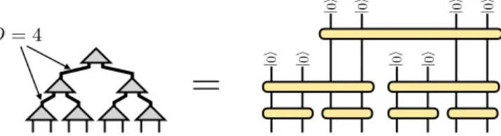
<latexit sha1_base64="uFbKRTBq720KdpN34ecdDTho5nE=">AAACtnicdVFNSwMxEE3X7/qtRy/BRfBUdougHoRCLx4VrArdpcym0zU0yS5JtlLW/gKvevdv+W9M1x7U1oHA4817eZNMkgtubBB81ryl5ZXVtfWN+ubW9s7u3v7BvckKzbDDMpHpxwQMCq6wY7kV+JhrBJkIfEiG7Wn/YYTa8Ezd2XGOsYRU8QFnYB11e9Xb84NGUBWdB+EM+GRWN7392kfUz1ghUVkmwJhuGOQ2LkFbzgRO6lFhMAc2hBS7DiqQaOKymnRCTxzTp4NMu6MsrdifjhKkMWOZOKUE+2T+9qbkol63sIOLuOQqLywq9h00KAS1GZ0+m/a5RmbF2AFgmrtZKXsCDcy6z6lHCp9ZJiWofhkN0U66YVxGqEyhcZpVvvhhpEGl7oGT3+pEw5w6EpXUD18WqKvrmwsN1Dn8Jv0nCUbpf0nO+MPldhr+3eA86DQbl43g9sxvtWfLXSdH5JickpCckxa5JjekQxhB8kreyLt36fU89NJvqVebeQ7Jr/LyL0OJ23s=</latexit><latexit sha1_base64="uFbKRTBq720KdpN34ecdDTho5nE=">AAACtnicdVFNSwMxEE3X7/qtRy/BRfBUdougHoRCLx4VrArdpcym0zU0yS5JtlLW/gKvevdv+W9M1x7U1oHA4817eZNMkgtubBB81ryl5ZXVtfWN+ubW9s7u3v7BvckKzbDDMpHpxwQMCq6wY7kV+JhrBJkIfEiG7Wn/YYTa8Ezd2XGOsYRU8QFnYB11e9Xb84NGUBWdB+EM+GRWN7392kfUz1ghUVkmwJhuGOQ2LkFbzgRO6lFhMAc2hBS7DiqQaOKymnRCTxzTp4NMu6MsrdifjhKkMWOZOKUE+2T+9qbkol63sIOLuOQqLywq9h00KAS1GZ0+m/a5RmbF2AFgmrtZKXsCDcy6z6lHCp9ZJiWofhkN0U66YVxGqEyhcZpVvvhhpEGl7oGT3+pEw5w6EpXUD18WqKvrmwsN1Dn8Jv0nCUbpf0nO+MPldhr+3eA86DQbl43g9sxvtWfLXSdH5JickpCckxa5JjekQxhB8kreyLt36fU89NJvqVebeQ7Jr/LyL0OJ23s=</latexit><latexit sha1_base64="uFbKRTBq720KdpN34ecdDTho5nE=">AAACtnicdVFNSwMxEE3X7/qtRy/BRfBUdougHoRCLx4VrArdpcym0zU0yS5JtlLW/gKvevdv+W9M1x7U1oHA4817eZNMkgtubBB81ryl5ZXVtfWN+ubW9s7u3v7BvckKzbDDMpHpxwQMCq6wY7kV+JhrBJkIfEiG7Wn/YYTa8Ezd2XGOsYRU8QFnYB11e9Xb84NGUBWdB+EM+GRWN7392kfUz1ghUVkmwJhuGOQ2LkFbzgRO6lFhMAc2hBS7DiqQaOKymnRCTxzTp4NMu6MsrdifjhKkMWOZOKUE+2T+9qbkol63sIOLuOQqLywq9h00KAS1GZ0+m/a5RmbF2AFgmrtZKXsCDcy6z6lHCp9ZJiWofhkN0U66YVxGqEyhcZpVvvhhpEGl7oGT3+pEw5w6EpXUD18WqKvrmwsN1Dn8Jv0nCUbpf0nO+MPldhr+3eA86DQbl43g9sxvtWfLXSdH5JickpCckxa5JjekQxhB8kreyLt36fU89NJvqVebeQ7Jr/LyL0OJ23s=</latexit>

FIG. 1. The quantum state of N qubits corresponding to

a tree tensor network (left) can be realized as a quantum

circuit acting onNqubits (right). The circuit is read from top

to bottom, with the yellow bars representing unitary gates.

The bond dimensionD connecting two nodes of the tensor

network is determined by number of qubitsV connecting two

sequential unitaries in the circuit, withD= 2V.

the parameters determining the unitary operations must be optimized for the specific machine learning task. Our approach is therefore conceptually related to the quan-tum variational eigensolver [23, 24] and to the quanquan-tum approximate optimization algorithms [25], where quan-tum circuit parameters are discovered with the help of an auxiliary classical algorithm.

The application of such hybrid quantum-classical al-gorithms to machine learning was recently investigated by several groups for labeling [26, 27] or generating data [28–30]. The proposals of Refs. 26, 27, 29, and 30 are re-lated to approaches we propose below, but consider very general classes of quantum circuits. This motivates the question: is there a subset of quantum circuits which are especially natural or advantageous for machine learn-ing tasks? Tensor network circuits might provide a com-pelling answer, for three main reasons:

1. Tensor network models could be implemented on

small, near-term quantum devices for input and output dimensions far exceeding the number of physical qubits. If the hardware permits the mea-surement of one of the qubits separately from the

(3)

others, then the number of physical qubits needed can be made to scale either logarithmically with the size of the processed data, or independently of the data size depending on the particular tensor network architecture. Models based on tensor net-works may also have an inherent resilience to noise. We explore both of these aspects in Section IV.

2. There is agradual crossoverfrom classically

sim-ulable tensor network circuits to circuits that re-quire a quantum computer to evaluate. With clas-sical resources, tensor network models already give very good results for supervised [12, 13, 15, 17]

and unsupervised [17, 19] learning tasks. The

same models—with the same dataset size and data dimension—can be used to initialize more expres-sive models requiring quantum hardware, mak-ing the optimization of the quantum-based model faster and more likely to succeed. Algorithmic im-provements in the classical setting can be readily transferred to the quantum setting as well.

3. There is a rich theoretical understanding of

the properties of tensor networks [2–4, 10, 31, 32], and their relative mathematical simplicity (involv-ing only linear operations) will likely facilitate fur-ther conceptual developments in the machine learn-ing context, such as interpretability and generaliza-tion. Properties of tensor networks, such as locality of correlations, may provide a favorable inductive bias for processing natural data [14]. One can prove rigorous bounds on the noise-resilience of quantum circuits based on tensor networks [33].

All of the experimental operations necessary to imple-ment tensor network circuits are available for near-term quantum hardware. The capabilities required are prepa-ration of product states; one- and two-qubit unitary op-erations; and measurement in the computational basis.

In what follows, we first describe our proposed frame-works for discriminative and generative learning tasks in Section II. Then we present results of a numerical exper-iment which demonstrates the feasibility of the approach using operations that could be carried out with an actual quantum device in Section III. We conclude by discussing how the learning approaches could be implemented with a small number of physical qubits and by addressing their resilience to noise in Section IV.

II. LEARNING WITH TENSOR NETWORK

QUANTUM CIRCUITS

The family of tensor networks we will consider—tree tensor networks and matrix product states—can always be realized precisely by a quantum circuit; see Fig. 1. Typically, the quantum circuits corresponding to tensor networks are carefully devised to make them efficient to prepare and manipulate with classical computers [34].

With increasing bond dimension, tree and matrix prod-uct state tensor gradually capture a wider range of states, which translates into more expressive and powerful mod-els within the context of machine learning.

For very large bond dimensions, tree and matrix prod-uct tensor networks can eventually encompass the en-tire state space. But when the bond dimensions become too high, the cost of the classical approach becomes pro-hibitive. By implementing tensor network circuits on quantum hardware instead, one could go far beyond the space of classically tractable models.

In this section, we first describe our tensor-network based proposal for performing discriminative tasks with quantum hardware. The goal of a discriminative model is to produce a specific output given a certain class of input; for example, assigning labels to images. Then we describe our proposal for generative tasks, where the goal is to generate samples from a probability distribution inferred from a data set. For more background on various types of machine learning tasks, see the recent review Ref. 35. For clarity of presentation, we shall make use of multi-qubit unitary operations in this work. However we recog-nize that in practice such unitaries must be implemented using a more limited set of few-qubit operations, such as the universal gate sets of one- and two-qubit opera-tors. Whether it is more productive to classically opti-mize over more general unitaries then “compile” these into few-qubit operations as a separate step, or to pa-rameterize the models in terms of fewer operations from the outset remains an interesting and important practical question for further work.

A. Discriminative Algorithm

To explain the discriminative tensor network frame-work that we propose here, assume that the input to

the algorithm takes the form of a vector ofN real

num-bersx= (x1, x2, . . . , xN), with each component

normal-ized such that xi ∈ [0,1]. For example, such an input

could correspond to a grayscale image withNpixels, with

individual entries encoding normalized grayscale values.

We map this vector x _∈ RN to a product state on N

qubits according to the feature map proposed in Ref. 13:

x _→ |Φ(x)_i= cos π 2x1 sin π₂x1 ⊗ cos π 2x2 sin π₂x2 ⊗ · · · ⊗ cos π 2xN sin π₂xN . (1) Such a state can be prepared by starting from the

com-putational basis state_|0_i⊗N, then applying a single qubit

unitary to each qubitn= 1,2, . . . , N.

The model we then propose can be seen as an iterative coarse-graining procedure that parameterizes a CPTP (completely positive trace preserving) map from an N-qubit input space to a small number of output N-qubits encoding the different possible class labels. The circuit

(4)

`

<latexit sha1_base64="4GGj+A11S286gICQQPOBvxkjn1g=">AAACuXicdVFNSwMxEE3Xr1o/q0cvwUXwVHaLoIIHwYtHBatCd5HZdNrGJtklySpl7V/wqkf/lv/G7NqD2joQeLx5L2+SSTLBjQ2Cz5q3sLi0vFJfbaytb2xubTd3bk2aa4YdlopU3ydgUHCFHcutwPtMI8hE4F0yuij7d0+oDU/VjR1nGEsYKN7nDGxJRSjEw7YftIKq6CwIp8An07p6aNY+ol7KconKMgHGdMMgs3EB2nImcNKIcoMZsBEMsOugAokmLqphJ/TAMT3aT7U7ytKK/ekoQBozlolTSrBD87dXkvN63dz2T+KCqyy3qNh3UD8X1Ka0fDntcY3MirEDwDR3s1I2BA3Muv9pRAqfWSolqF4RjdBOumFcRKhMrrHMKl78MNKgBu6Bk9/qRMOMOhKV1A9f5qir69tzDdQ5/Db9JwmeBv8lOeMPl9tp+HeDs6DTbp22gusj//xiutw62SP75JCE5Jick0tyRTqEkSF5JW/k3TvzEm/oPX5LvdrUs0t+lWe+AN6U3PU=</latexit>

=<latexit sha1_base64="NRrUKEqzmqotoFv+0mTMVdMJHg8=">AAACtnicdVFNSwMxEE3X7/qtRy/BRfBUdougHpSCF48KVoXuUmbT6RqaZJckq5Rtf4FXvfu3/Demaw9q60Dg8ea9vEkmyQU3Ngg+a97C4tLyyupafX1jc2t7Z3fv3mSFZthmmcj0YwIGBVfYttwKfMw1gkwEPiSDq0n/4Rm14Zm6s8McYwmp4n3OwDrq9qK74weNoCo6C8Ip8Mm0brq7tY+ol7FCorJMgDGdMMhtXIK2nAkc16PCYA5sACl2HFQg0cRlNemYHjmmR/uZdkdZWrE/HSVIY4YycUoJ9sn87U3Ieb1OYftncclVXlhU7DuoXwhqMzp5Nu1xjcyKoQPANHezUvYEGph1n1OPFL6wTEpQvTIaoB13wriMUJlC4ySrHPlhpEGl7oHj3+pEw4w6EpXUD0dz1NX1zbkG6hx+k/6TBM/pf0nO+MPldhr+3eAsaDcb543g9sRvXU6Xu0oOyCE5JiE5JS1yTW5ImzCC5JW8kXfv3Ot66KXfUq829eyTX+XlX0II23Y=</latexit><latexit sha1_base64="NRrUKEqzmqotoFv+0mTMVdMJHg8=">AAACtnicdVFNSwMxEE3X7/qtRy/BRfBUdougHpSCF48KVoXuUmbT6RqaZJckq5Rtf4FXvfu3/Demaw9q60Dg8ea9vEkmyQU3Ngg+a97C4tLyyupafX1jc2t7Z3fv3mSFZthmmcj0YwIGBVfYttwKfMw1gkwEPiSDq0n/4Rm14Zm6s8McYwmp4n3OwDrq9qK74weNoCo6C8Ip8Mm0brq7tY+ol7FCorJMgDGdMMhtXIK2nAkc16PCYA5sACl2HFQg0cRlNemYHjmmR/uZdkdZWrE/HSVIY4YycUoJ9sn87U3Ieb1OYftncclVXlhU7DuoXwhqMzp5Nu1xjcyKoQPANHezUvYEGph1n1OPFL6wTEpQvTIaoB13wriMUJlC4ySrHPlhpEGl7oHj3+pEw4w6EpXUD0dz1NX1zbkG6hx+k/6TBM/pf0nO+MPldhr+3eAsaDcb543g9sRvXU6Xu0oOyCE5JiE5JS1yTW5ImzCC5JW8kXfv3Ot66KXfUq829eyTX+XlX0II23Y=</latexit><latexit sha1_base64="NRrUKEqzmqotoFv+0mTMVdMJHg8=">AAACtnicdVFNSwMxEE3X7/qtRy/BRfBUdougHpSCF48KVoXuUmbT6RqaZJckq5Rtf4FXvfu3/Demaw9q60Dg8ea9vEkmyQU3Ngg+a97C4tLyyupafX1jc2t7Z3fv3mSFZthmmcj0YwIGBVfYttwKfMw1gkwEPiSDq0n/4Rm14Zm6s8McYwmp4n3OwDrq9qK74weNoCo6C8Ip8Mm0brq7tY+ol7FCorJMgDGdMMhtXIK2nAkc16PCYA5sACl2HFQg0cRlNemYHjmmR/uZdkdZWrE/HSVIY4YycUoJ9sn87U3Ieb1OYftncclVXlhU7DuoXwhqMzp5Nu1xjcyKoQPANHezUvYEGph1n1OPFL6wTEpQvTIaoB13wriMUJlC4ySrHPlhpEGl7oHj3+pEw4w6EpXUD0dz1NX1zbkG6hx+k/6TBM/pf0nO+MPldhr+3eAsaDcb543g9sRvXU6Xu0oOyCE5JiE5JS1yTW5ImzCC5JW8kXfv3Ot66KXfUq829eyTX+XlX0II23Y=</latexit> prepared input qubit

=<latexit sha1_base64="NRrUKEqzmqotoFv+0mTMVdMJHg8=">AAACtnicdVFNSwMxEE3X7/qtRy/BRfBUdougHpSCF48KVoXuUmbT6RqaZJckq5Rtf4FXvfu3/Demaw9q60Dg8ea9vEkmyQU3Ngg+a97C4tLyyupafX1jc2t7Z3fv3mSFZthmmcj0YwIGBVfYttwKfMw1gkwEPiSDq0n/4Rm14Zm6s8McYwmp4n3OwDrq9qK74weNoCo6C8Ip8Mm0brq7tY+ol7FCorJMgDGdMMhtXIK2nAkc16PCYA5sACl2HFQg0cRlNemYHjmmR/uZdkdZWrE/HSVIY4YycUoJ9sn87U3Ieb1OYftncclVXlhU7DuoXwhqMzp5Nu1xjcyKoQPANHezUvYEGph1n1OPFL6wTEpQvTIaoB13wriMUJlC4ySrHPlhpEGl7oHj3+pEw4w6EpXUD0dz1NX1zbkG6hx+k/6TBM/pf0nO+MPldhr+3eAsaDcb543g9sRvXU6Xu0oOyCE5JiE5JS1yTW5ImzCC5JW8kXfv3Ot66KXfUq829eyTX+XlX0II23Y=</latexit><latexit sha1_base64="NRrUKEqzmqotoFv+0mTMVdMJHg8=">AAACtnicdVFNSwMxEE3X7/qtRy/BRfBUdougHpSCF48KVoXuUmbT6RqaZJckq5Rtf4FXvfu3/Demaw9q60Dg8ea9vEkmyQU3Ngg+a97C4tLyyupafX1jc2t7Z3fv3mSFZthmmcj0YwIGBVfYttwKfMw1gkwEPiSDq0n/4Rm14Zm6s8McYwmp4n3OwDrq9qK74weNoCo6C8Ip8Mm0brq7tY+ol7FCorJMgDGdMMhtXIK2nAkc16PCYA5sACl2HFQg0cRlNemYHjmmR/uZdkdZWrE/HSVIY4YycUoJ9sn87U3Ieb1OYftncclVXlhU7DuoXwhqMzp5Nu1xjcyKoQPANHezUvYEGph1n1OPFL6wTEpQvTIaoB13wriMUJlC4ySrHPlhpEGl7oHj3+pEw4w6EpXUD0dz1NX1zbkG6hx+k/6TBM/pf0nO+MPldhr+3eAsaDcb543g9sRvXU6Xu0oOyCE5JiE5JS1yTW5ImzCC5JW8kXfv3Ot66KXfUq829eyTX+XlX0II23Y=</latexit><latexit sha1_base64="NRrUKEqzmqotoFv+0mTMVdMJHg8=">AAACtnicdVFNSwMxEE3X7/qtRy/BRfBUdougHpSCF48KVoXuUmbT6RqaZJckq5Rtf4FXvfu3/Demaw9q60Dg8ea9vEkmyQU3Ngg+a97C4tLyyupafX1jc2t7Z3fv3mSFZthmmcj0YwIGBVfYttwKfMw1gkwEPiSDq0n/4Rm14Zm6s8McYwmp4n3OwDrq9qK74weNoCo6C8Ip8Mm0brq7tY+ol7FCorJMgDGdMMhtXIK2nAkc16PCYA5sACl2HFQg0cRlNemYHjmmR/uZdkdZWrE/HSVIY4YycUoJ9sn87U3Ieb1OYftncclVXlhU7DuoXwhqMzp5Nu1xjcyKoQPANHezUvYEGph1n1OPFL6wTEpQvTIaoB13wriMUJlC4ySrHPlhpEGl7oHj3+pEw4w6EpXUD0dz1NX1zbkG6hx+k/6TBM/pf0nO+MPldhr+3eAsaDcb543g9sRvXU6Xu0oOyCE5JiE5JS1yTW5ImzCC5JW8kXfv3Ot66KXfUq829eyTX+XlX0II23Y=</latexit> unitary transformation =<latexit sha1_base64="NRrUKEqzmqotoFv+0mTMVdMJHg8=">AAACtnicdVFNSwMxEE3X7/qtRy/BRfBUdougHpSCF48KVoXuUmbT6RqaZJckq5Rtf4FXvfu3/Demaw9q60Dg8ea9vEkmyQU3Ngg+a97C4tLyyupafX1jc2t7Z3fv3mSFZthmmcj0YwIGBVfYttwKfMw1gkwEPiSDq0n/4Rm14Zm6s8McYwmp4n3OwDrq9qK74weNoCo6C8Ip8Mm0brq7tY+ol7FCorJMgDGdMMhtXIK2nAkc16PCYA5sACl2HFQg0cRlNemYHjmmR/uZdkdZWrE/HSVIY4YycUoJ9sn87U3Ieb1OYftncclVXlhU7DuoXwhqMzp5Nu1xjcyKoQPANHezUvYEGph1n1OPFL6wTEpQvTIaoB13wriMUJlC4ySrHPlhpEGl7oHj3+pEw4w6EpXUD0dz1NX1zbkG6hx+k/6TBM/pf0nO+MPldhr+3eAsaDcb543g9sRvXU6Xu0oOyCE5JiE5JS1yTW5ImzCC5JW8kXfv3Ot66KXfUq829eyTX+XlX0II23Y=</latexit><latexit sha1_base64="NRrUKEqzmqotoFv+0mTMVdMJHg8=">AAACtnicdVFNSwMxEE3X7/qtRy/BRfBUdougHpSCF48KVoXuUmbT6RqaZJckq5Rtf4FXvfu3/Demaw9q60Dg8ea9vEkmyQU3Ngg+a97C4tLyyupafX1jc2t7Z3fv3mSFZthmmcj0YwIGBVfYttwKfMw1gkwEPiSDq0n/4Rm14Zm6s8McYwmp4n3OwDrq9qK74weNoCo6C8Ip8Mm0brq7tY+ol7FCorJMgDGdMMhtXIK2nAkc16PCYA5sACl2HFQg0cRlNemYHjmmR/uZdkdZWrE/HSVIY4YycUoJ9sn87U3Ieb1OYftncclVXlhU7DuoXwhqMzp5Nu1xjcyKoQPANHezUvYEGph1n1OPFL6wTEpQvTIaoB13wriMUJlC4ySrHPlhpEGl7oHj3+pEw4w6EpXUD0dz1NX1zbkG6hx+k/6TBM/pf0nO+MPldhr+3eAsaDcb543g9sRvXU6Xu0oOyCE5JiE5JS1yTW5ImzCC5JW8kXfv3Ot66KXfUq829eyTX+XlX0II23Y=</latexit><latexit sha1_base64="NRrUKEqzmqotoFv+0mTMVdMJHg8=">AAACtnicdVFNSwMxEE3X7/qtRy/BRfBUdougHpSCF48KVoXuUmbT6RqaZJckq5Rtf4FXvfu3/Demaw9q60Dg8ea9vEkmyQU3Ngg+a97C4tLyyupafX1jc2t7Z3fv3mSFZthmmcj0YwIGBVfYttwKfMw1gkwEPiSDq0n/4Rm14Zm6s8McYwmp4n3OwDrq9qK74weNoCo6C8Ip8Mm0brq7tY+ol7FCorJMgDGdMMhtXIK2nAkc16PCYA5sACl2HFQg0cRlNemYHjmmR/uZdkdZWrE/HSVIY4YycUoJ9sn87U3Ieb1OYftncclVXlhU7DuoXwhqMzp5Nu1xjcyKoQPANHezUvYEGph1n1OPFL6wTEpQvTIaoB13wriMUJlC4ySrHPlhpEGl7oHj3+pEw4w6EpXUD0dz1NX1zbkG6hx+k/6TBM/pf0nO+MPldhr+3eAsaDcb543g9sRvXU6Xu0oOyCE5JiE5JS1yTW5ImzCC5JW8kXfv3Ot66KXfUq829eyTX+XlX0II23Y=</latexit> traced/unobserved qubit

=<latexit sha1_base64="NRrUKEqzmqotoFv+0mTMVdMJHg8=">AAACtnicdVFNSwMxEE3X7/qtRy/BRfBUdougHpSCF48KVoXuUmbT6RqaZJckq5Rtf4FXvfu3/Demaw9q60Dg8ea9vEkmyQU3Ngg+a97C4tLyyupafX1jc2t7Z3fv3mSFZthmmcj0YwIGBVfYttwKfMw1gkwEPiSDq0n/4Rm14Zm6s8McYwmp4n3OwDrq9qK74weNoCo6C8Ip8Mm0brq7tY+ol7FCorJMgDGdMMhtXIK2nAkc16PCYA5sACl2HFQg0cRlNemYHjmmR/uZdkdZWrE/HSVIY4YycUoJ9sn87U3Ieb1OYftncclVXlhU7DuoXwhqMzp5Nu1xjcyKoQPANHezUvYEGph1n1OPFL6wTEpQvTIaoB13wriMUJlC4ySrHPlhpEGl7oHj3+pEw4w6EpXUD0dz1NX1zbkG6hx+k/6TBM/pf0nO+MPldhr+3eAsaDcb543g9sRvXU6Xu0oOyCE5JiE5JS1yTW5ImzCC5JW8kXfv3Ot66KXfUq829eyTX+XlX0II23Y=</latexit><latexit sha1_base64="NRrUKEqzmqotoFv+0mTMVdMJHg8=">AAACtnicdVFNSwMxEE3X7/qtRy/BRfBUdougHpSCF48KVoXuUmbT6RqaZJckq5Rtf4FXvfu3/Demaw9q60Dg8ea9vEkmyQU3Ngg+a97C4tLyyupafX1jc2t7Z3fv3mSFZthmmcj0YwIGBVfYttwKfMw1gkwEPiSDq0n/4Rm14Zm6s8McYwmp4n3OwDrq9qK74weNoCo6C8Ip8Mm0brq7tY+ol7FCorJMgDGdMMhtXIK2nAkc16PCYA5sACl2HFQg0cRlNemYHjmmR/uZdkdZWrE/HSVIY4YycUoJ9sn87U3Ieb1OYftncclVXlhU7DuoXwhqMzp5Nu1xjcyKoQPANHezUvYEGph1n1OPFL6wTEpQvTIaoB13wriMUJlC4ySrHPlhpEGl7oHj3+pEw4w6EpXUD0dz1NX1zbkG6hx+k/6TBM/pf0nO+MPldhr+3eAsaDcb543g9sRvXU6Xu0oOyCE5JiE5JS1yTW5ImzCC5JW8kXfv3Ot66KXfUq829eyTX+XlX0II23Y=</latexit><latexit sha1_base64="NRrUKEqzmqotoFv+0mTMVdMJHg8=">AAACtnicdVFNSwMxEE3X7/qtRy/BRfBUdougHpSCF48KVoXuUmbT6RqaZJckq5Rtf4FXvfu3/Demaw9q60Dg8ea9vEkmyQU3Ngg+a97C4tLyyupafX1jc2t7Z3fv3mSFZthmmcj0YwIGBVfYttwKfMw1gkwEPiSDq0n/4Rm14Zm6s8McYwmp4n3OwDrq9qK74weNoCo6C8Ip8Mm0brq7tY+ol7FCorJMgDGdMMhtXIK2nAkc16PCYA5sACl2HFQg0cRlNemYHjmmR/uZdkdZWrE/HSVIY4YycUoJ9sn87U3Ieb1OYftncclVXlhU7DuoXwhqMzp5Nu1xjcyKoQPANHezUvYEGph1n1OPFL6wTEpQvTIaoB13wriMUJlC4ySrHPlhpEGl7oHj3+pEw4w6EpXUD0dz1NX1zbkG6hx+k/6TBM/pf0nO+MPldhr+3eAsaDcb543g9sRvXU6Xu0oOyCE5JiE5JS1yTW5ImzCC5JW8kXfv3Ot66KXfUq829eyTX+XlX0II23Y=</latexit> measured/observed qubit

(a) (b) <latexit sha1_base64="r/Np+kwPs3sdsXNzIemkxgxIqiQ=">AAACvnicdVFNTxsxEHUWCjQUSuixF4sVEqdoN0KCHpBSceFIpaaAsqto1pksVvyxsr1AtORX9Eql/q3+mzqbHAIJI1l6evOe39iTFYJbF0X/GsHG5oet7Z2Pzd1Pe/ufD1qHv6wuDcMe00Kb2wwsCq6w57gTeFsYBJkJvMnGl7P+zQMay7X66SYFphJyxUecgfPUXTFIUAh6QQcHYdSO6qKrIF6AkCzqetBq/E2GmpUSlWMCrO3HUeHSCozjTOC0mZQWC2BjyLHvoQKJNq3qiaf02DNDOtLGH+VozS47KpDWTmTmlRLcvX3bm5Hrev3Sjc7TiquidKjYPGhUCuo0nT2fDrlB5sTEA2CG+1kpuwcDzPlPaiYKH5mWEtSwSsbopv04rRJUtjQ4y6qewzgxoHL/wOlrdWZgRZ2IWhrGz2vU9fWdtQbqHWGHvpMED/l7Sd645PI7jd9ucBX0Ou1v7ejHadi9XCx3h3wlR+SExOSMdMkVuSY9wogkv8kL+RN8D/JABnouDRoLzxfyqoKn/6k13nM=</latexit><latexit sha1_base64="r/Np+kwPs3sdsXNzIemkxgxIqiQ=">AAACvnicdVFNTxsxEHUWCjQUSuixF4sVEqdoN0KCHpBSceFIpaaAsqto1pksVvyxsr1AtORX9Eql/q3+mzqbHAIJI1l6evOe39iTFYJbF0X/GsHG5oet7Z2Pzd1Pe/ufD1qHv6wuDcMe00Kb2wwsCq6w57gTeFsYBJkJvMnGl7P+zQMay7X66SYFphJyxUecgfPUXTFIUAh6QQcHYdSO6qKrIF6AkCzqetBq/E2GmpUSlWMCrO3HUeHSCozjTOC0mZQWC2BjyLHvoQKJNq3qiaf02DNDOtLGH+VozS47KpDWTmTmlRLcvX3bm5Hrev3Sjc7TiquidKjYPGhUCuo0nT2fDrlB5sTEA2CG+1kpuwcDzPlPaiYKH5mWEtSwSsbopv04rRJUtjQ4y6qewzgxoHL/wOlrdWZgRZ2IWhrGz2vU9fWdtQbqHWGHvpMED/l7Sd645PI7jd9ucBX0Ou1v7ejHadi9XCx3h3wlR+SExOSMdMkVuSY9wogkv8kL+RN8D/JABnouDRoLzxfyqoKn/6k13nM=</latexit><latexit sha1_base64="r/Np+kwPs3sdsXNzIemkxgxIqiQ=">AAACvnicdVFNTxsxEHUWCjQUSuixF4sVEqdoN0KCHpBSceFIpaaAsqto1pksVvyxsr1AtORX9Eql/q3+mzqbHAIJI1l6evOe39iTFYJbF0X/GsHG5oet7Z2Pzd1Pe/ufD1qHv6wuDcMe00Kb2wwsCq6w57gTeFsYBJkJvMnGl7P+zQMay7X66SYFphJyxUecgfPUXTFIUAh6QQcHYdSO6qKrIF6AkCzqetBq/E2GmpUSlWMCrO3HUeHSCozjTOC0mZQWC2BjyLHvoQKJNq3qiaf02DNDOtLGH+VozS47KpDWTmTmlRLcvX3bm5Hrev3Sjc7TiquidKjYPGhUCuo0nT2fDrlB5sTEA2CG+1kpuwcDzPlPaiYKH5mWEtSwSsbopv04rRJUtjQ4y6qewzgxoHL/wOlrdWZgRZ2IWhrGz2vU9fWdtQbqHWGHvpMED/l7Sd645PI7jd9ucBX0Ou1v7ejHadi9XCx3h3wlR+SExOSMdMkVuSY9wogkv8kL+RN8D/JABnouDRoLzxfyqoKn/6k13nM=</latexit>

p

`

=

`

<latexit sha1_base64="4GGj+A11S286gICQQPOBvxkjn1g=">AAACuXicdVFNSwMxEE3Xr1o/q0cvwUXwVHaLoIIHwYtHBatCd5HZdNrGJtklySpl7V/wqkf/lv/G7NqD2joQeLx5L2+SSTLBjQ2Cz5q3sLi0vFJfbaytb2xubTd3bk2aa4YdlopU3ydgUHCFHcutwPtMI8hE4F0yuij7d0+oDU/VjR1nGEsYKN7nDGxJRSjEw7YftIKq6CwIp8An07p6aNY+ol7KconKMgHGdMMgs3EB2nImcNKIcoMZsBEMsOugAokmLqphJ/TAMT3aT7U7ytKK/ekoQBozlolTSrBD87dXkvN63dz2T+KCqyy3qNh3UD8X1Ka0fDntcY3MirEDwDR3s1I2BA3Muv9pRAqfWSolqF4RjdBOumFcRKhMrrHMKl78MNKgBu6Bk9/qRMOMOhKV1A9f5qir69tzDdQ5/Db9JwmeBv8lOeMPl9tp+HeDs6DTbp22gusj//xiutw62SP75JCE5Jick0tyRTqEkSF5JW/k3TvzEm/oPX5LvdrUs0t+lWe+AN6U3PU=</latexit>

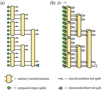
FIG. 2. Discriminative tree tensor network model

architec-ture, showing an example in which V = 2 qubits connect

different subtrees. Figure (a) shows the model implementa-tion as a quantum circuit. Circles indicate inputs prepared in a product state as in Eq. 1; hash marks indicate qubits that remain unobserved past a certain point in the circuit. A particular pre-determined qubit is sampled (square symbol) and its distribution serves as the output of the model. Figure (b) shows the tensor network diagram for the reduced density matrix of the output qubit.

takes the form of a tree, with V qubit lines connecting

each subtree to the rest of the circuit. We call such qubit lines “virtual qubits” to connect with the terminology of tensor networks, where tensor indices internal to the

net-work are called virtual indices. A larger V can capture

a larger set of functions, just as a tensor network with a sufficiently large bond dimension can parameterize any N-index tensor.

At each step, we take V of the qubits resulting from

one of the unitary operations of the previous step, or

sub-tree, andV from another subtree and act on them with

another parameterized unitary transformation (possibly

together with some ancilla qubits—not shown). ThenV

of the qubits are discarded, while the otherV proceed to

the next node of the tree, that is, the next step of the

FIG. 3. The connectivity of nodes of our tree network model, as it would be applied to a 4x4 image. Each step coarse-grains in either the horizontal or the vertical directions, and these steps alternate.

circuit. In our classical simulations we trace over all dis-carded qubits, while on a quantum computer, we would be free to ignore or reset such qubits.

Once all unitary operations defining the circuit have been carried out, one or more qubits serve as the output qubits. (Which qubits are outputs is designated ahead of time.) The most probable state of the output qubits determines the prediction of the model, that is, the la-bel the model assigns to the input. To determine the most probable state of the output qubits, one performs repeated evaluations of the circuit for the same input in order to estimate their probability distribution in the computational basis.

We show the quantum circuit of our proposed proce-dure in Fig. 2. In the case of image classification, it is natural to always group input qubits based on pixels coming from nearby regions of the image, with a tree structure illustrated schematically in Fig. 3.

A closely related family of models can be devised based on matrix product states. An example is illustrated in

Fig. 4 showing the case ofV = 2. Matrix product states

(MPS) can be viewed as maximally unbalanced trees, and differ from the binary tree models described above in that

after each unitary operation on 2V inputs only one set

ofV qubits are passed to the next node of the network.

Such models are likely a better fit for data that has a one-dimensional pattern of correlations, such as time-series, language, or audio data.

B. Generative Algorithm

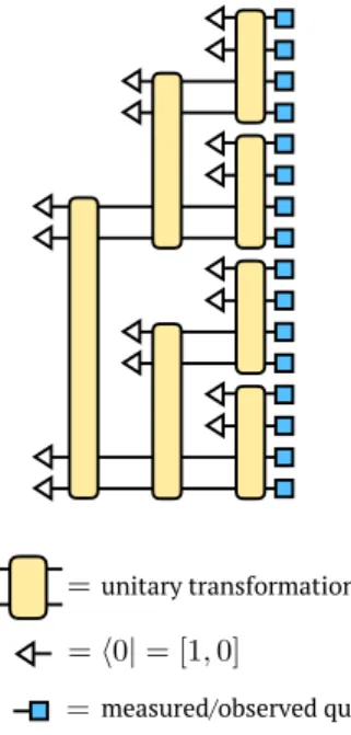
The generative algorithm we propose is nearly the re-verse of the discriminative algorithm, in terms of its cir-cuit architecture. The algorithm produces random sam-ples by first preparing a quantum state then measuring it in the computational basis, putting it within the family of

FIG. 4. Discriminative tensor network model for the case

of a matrix product state (MPS) architecture with V = 2

qubits connecting each subtree. The symbols have the same meaning as in Fig. 2. An MPS can be viewed as a maximally unbalanced tree.

(5)

algorithms recently dubbed “Born machines” [19, 28, 29]. But rather than preparing a completely general state, we shall consider specific patterns of state preparation corresponding to tree and matrix product state tensor networks. This provides the advantages discussed in the introduction, such as connections to classical tensor net-work models and the ability to reduce the number of physical qubits required, which will be discussed further in Section IV.

The generative algorithm based on a tree tensor

net-work (shown in Fig. 5) begins by preparing 2V qubits

in a reference computational basis state_h0_|⊗2V, then

en-tangling these qubits by unitary operations. Another set

of 2V qubits are prepared in the state h0|⊗2V. Half of

these are grouped with the firstV entangled qubits, and

half with the secondV entangled qubits. Two more

uni-tary operations are applied to each new grouping of 2V

qubits; the outputs are now split into four groups; and the process repeats for each group. The process ends when the total number of qubits processed reaches the size of the output one wants to generate.

Once all unitaries acting on a certain qubit have been applied, this qubit can be measured. The measured out-put of all of the qubits in the comout-putational basis

repre-=

<latexit sha1_base64="NRrUKEqzmqotoFv+0mTMVdMJHg8=">AAACtnicdVFNSwMxEE3X7/qtRy/BRfBUdougHpSCF48KVoXuUmbT6RqaZJckq5Rtf4FXvfu3/Demaw9q60Dg8ea9vEkmyQU3Ngg+a97C4tLyyupafX1jc2t7Z3fv3mSFZthmmcj0YwIGBVfYttwKfMw1gkwEPiSDq0n/4Rm14Zm6s8McYwmp4n3OwDrq9qK74weNoCo6C8Ip8Mm0brq7tY+ol7FCorJMgDGdMMhtXIK2nAkc16PCYA5sACl2HFQg0cRlNemYHjmmR/uZdkdZWrE/HSVIY4YycUoJ9sn87U3Ieb1OYftncclVXlhU7DuoXwhqMzp5Nu1xjcyKoQPANHezUvYEGph1n1OPFL6wTEpQvTIaoB13wriMUJlC4ySrHPlhpEGl7oHj3+pEw4w6EpXUD0dz1NX1zbkG6hx+k/6TBM/pf0nO+MPldhr+3eAsaDcb543g9sRvXU6Xu0oOyCE5JiE5JS1yTW5ImzCC5JW8kXfv3Ot66KXfUq829eyTX+XlX0II23Y=</latexit>

<latexit sha1_base64="NRrUKEqzmqotoFv+0mTMVdMJHg8=">AAACtnicdVFNSwMxEE3X7/qtRy/BRfBUdougHpSCF48KVoXuUmbT6RqaZJckq5Rtf4FXvfu3/Demaw9q60Dg8ea9vEkmyQU3Ngg+a97C4tLyyupafX1jc2t7Z3fv3mSFZthmmcj0YwIGBVfYttwKfMw1gkwEPiSDq0n/4Rm14Zm6s8McYwmp4n3OwDrq9qK74weNoCo6C8Ip8Mm0brq7tY+ol7FCorJMgDGdMMhtXIK2nAkc16PCYA5sACl2HFQg0cRlNemYHjmmR/uZdkdZWrE/HSVIY4YycUoJ9sn87U3Ieb1OYftncclVXlhU7DuoXwhqMzp5Nu1xjcyKoQPANHezUvYEGph1n1OPFL6wTEpQvTIaoB13wriMUJlC4ySrHPlhpEGl7oHj3+pEw4w6EpXUD0dz1NX1zbkG6hx+k/6TBM/pf0nO+MPldhr+3eAsaDcb543g9sRvXU6Xu0oOyCE5JiE5JS1yTW5ImzCC5JW8kXfv3Ot66KXfUq829eyTX+XlX0II23Y=</latexit> unitary transformation

=<latexit sha1_base64="NRrUKEqzmqotoFv+0mTMVdMJHg8=">AAACtnicdVFNSwMxEE3X7/qtRy/BRfBUdougHpSCF48KVoXuUmbT6RqaZJckq5Rtf4FXvfu3/Demaw9q60Dg8ea9vEkmyQU3Ngg+a97C4tLyyupafX1jc2t7Z3fv3mSFZthmmcj0YwIGBVfYttwKfMw1gkwEPiSDq0n/4Rm14Zm6s8McYwmp4n3OwDrq9qK74weNoCo6C8Ip8Mm0brq7tY+ol7FCorJMgDGdMMhtXIK2nAkc16PCYA5sACl2HFQg0cRlNemYHjmmR/uZdkdZWrE/HSVIY4YycUoJ9sn87U3Ieb1OYftncclVXlhU7DuoXwhqMzp5Nu1xjcyKoQPANHezUvYEGph1n1OPFL6wTEpQvTIaoB13wriMUJlC4ySrHPlhpEGl7oHj3+pEw4w6EpXUD0dz1NX1zbkG6hx+k/6TBM/pf0nO+MPldhr+3eAsaDcb543g9sRvXU6Xu0oOyCE5JiE5JS1yTW5ImzCC5JW8kXfv3Ot66KXfUq829eyTX+XlX0II23Y=</latexit><latexit sha1_base64="NRrUKEqzmqotoFv+0mTMVdMJHg8=">AAACtnicdVFNSwMxEE3X7/qtRy/BRfBUdougHpSCF48KVoXuUmbT6RqaZJckq5Rtf4FXvfu3/Demaw9q60Dg8ea9vEkmyQU3Ngg+a97C4tLyyupafX1jc2t7Z3fv3mSFZthmmcj0YwIGBVfYttwKfMw1gkwEPiSDq0n/4Rm14Zm6s8McYwmp4n3OwDrq9qK74weNoCo6C8Ip8Mm0brq7tY+ol7FCorJMgDGdMMhtXIK2nAkc16PCYA5sACl2HFQg0cRlNemYHjmmR/uZdkdZWrE/HSVIY4YycUoJ9sn87U3Ieb1OYftncclVXlhU7DuoXwhqMzp5Nu1xjcyKoQPANHezUvYEGph1n1OPFL6wTEpQvTIaoB13wriMUJlC4ySrHPlhpEGl7oHj3+pEw4w6EpXUD0dz1NX1zbkG6hx+k/6TBM/pf0nO+MPldhr+3eAsaDcb543g9sRvXU6Xu0oOyCE5JiE5JS1yTW5ImzCC5JW8kXfv3Ot66KXfUq829eyTX+XlX0II23Y=</latexit><latexit sha1_base64="NRrUKEqzmqotoFv+0mTMVdMJHg8=">AAACtnicdVFNSwMxEE3X7/qtRy/BRfBUdougHpSCF48KVoXuUmbT6RqaZJckq5Rtf4FXvfu3/Demaw9q60Dg8ea9vEkmyQU3Ngg+a97C4tLyyupafX1jc2t7Z3fv3mSFZthmmcj0YwIGBVfYttwKfMw1gkwEPiSDq0n/4Rm14Zm6s8McYwmp4n3OwDrq9qK74weNoCo6C8Ip8Mm0brq7tY+ol7FCorJMgDGdMMhtXIK2nAkc16PCYA5sACl2HFQg0cRlNemYHjmmR/uZdkdZWrE/HSVIY4YycUoJ9sn87U3Ieb1OYftncclVXlhU7DuoXwhqMzp5Nu1xjcyKoQPANHezUvYEGph1n1OPFL6wTEpQvTIaoB13wriMUJlC4ySrHPlhpEGl7oHj3+pEw4w6EpXUD0dz1NX1zbkG6hx+k/6TBM/pf0nO+MPldhr+3eAsaDcb543g9sRvXU6Xu0oOyCE5JiE5JS1yTW5ImzCC5JW8kXfv3Ot66KXfUq829eyTX+XlX0II23Y=</latexit> measured/observed qubit

=_h0_|= [1,0]

<latexit sha1_base64="mA1wXIdvp6YroCJlfjHpPKbzkVs=">AAACyXicdVHBThsxEHUWaNNQSoBjLxYrJA5VtBsh0R6oInHh0AOVGkDaXUWzziRYsb0r20tJlz3xH4hb+SX+BmfJAUgYydLTm/f87Jk0F9zYIHhseCurax8+Nj+11j9vfNlsb22fmazQDPssE5m+SMGg4Ar7lluBF7lGkKnA83RyPOufX6E2PFN/7DTHRMJY8RFnYB01aG8f0TjVUAYVPaJR+I0GyaDtB52gLroIwjnwybxOB1uN+3iYsUKiskyAMVEY5DYpQVvOBFatuDCYA5vAGCMHFUg0SVk/vqJ7jhnSUabdUZbW7EtHCdKYqUydUoK9NG97M3JZLyrs6HtScpUXFhV7DhoVgtqMziZBh1wjs2LqADDN3VspuwQNzLp5tWKFf1kmJahhGU/QVlGYlDEqU2icZZU3fhhrUGP3weq12s1zQR2LWuqHN0vU9fXdpQbqHH6XvpMEV+P3kpzxhcvtNHy7wUXQ73Z+dILfB37v53y5TfKV7JJ9EpJD0iMn5JT0CSPX5I78Jw/eL097196/Z6nXmHt2yKvybp8AfUHhDA==</latexit>

FIG. 5. Generative tree tensor network model architecture,

showing a case with V = 2 qubits connecting each subtree.

To sample from the model, qubits are prepared in a reference

computational basis stateh0|(left-hand side of circuit). Then

2V qubits are entangled via unitary operations at each layer

of the tree as shown. The qubits are measured at the points in the circuit labeled by square symbols (right-hand side of circuit), and the results of these measurements provides the output of the model. While all qubits could be entangled before being measured, we discuss in Section IV the possi-bility performing opportunistic measurements to reduce the physical qubit overhead.

sents one sample from the generative model.

We illustrate our proposed generative approach for the

case ofV = 2 and binary outputs in Fig. 5. As in the

discriminative case, one can also devise an MPS based generative algorithm more suitable for one-dimensional data. The circuit for such an algorithm is shown in Fig. 6.

III. NUMERICAL EXPERIMENTS

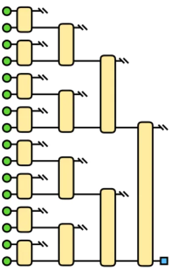
To show the feasibility of implementing our proposal on a near-term quantum device, we trained a discriminative model based on a tree tensor network for a supervised learning task, namely labeling image data. The specific network architecture we used is shown as a quantum cir-cuit in Fig. 7. When viewed as a tensor network, this

model has a bond dimension ofD= 2. This stems from

the fact that after each unitary operation entangles two qubits, only one of the qubits is acted on at the next scale (next step of the circuit).

A. Loss Function

Our eventual goal is to select the parameters of our circuit such that we can confidently assign the correct label to a new piece of data by running our circuit a small number of times. To this end, we choose the loss function which we want to minimize starting with the

following definitions. LetΛbe the model parameters; d

be an element of the training data set; and letp`(Λ,x) be

the probability of the model to output a label`for a given

inputx. Because we consider the setting of supervised

learning, the correct labels are known for the training set

inputs, and define`xto be the correct label for the input

x. Now define

plargest false(Λ,x) = max

`6=`x

h

p`(Λ,x)

i

(2)

FIG. 6. Generative tensor network model for the case of a

matrix product state (MPS) architecture withV = 2 qubits

connecting each unitary. The symbols have the same meaning as in Fig. 5.

(6)

FIG. 7. Model architecture used in the experiments of Sec-tion III, which is a special case of the model of Fig. 2 with one virtual qubit connecting each subtree. For illustration purposes we show a model with 16 inputs and 4 layers above, whereas the actual model used in the experiments had 64 in-puts and 6 layers.

as the probability of the incorrect output state which has the highest probability of being observed. Then, define

the loss function for a single inputxto be

L(Λ,x) = max(plargest false(Λ,x)₋p`x(Λ,x) +λ,0)

η_,

(3) and the total loss function to be

L(Λ) = 1

|data|

X

x∈data

L(Λ,x). (4)

The “hyper-parameters” λ and η are to be chosen to

give good empirical performance on a validation data set. Essentially, we assign a penalty for each element of the training set where the gap between probability of assign-ing the true label and the probability of assignassign-ing the

most likely incorrect label is less thanλ. This loss

func-tion allows us to concentrate our efforts during training on making sure that we are likely to assign the correct label after taking the majority vote of several executions of the model, rather than trying to force the model to always output the correct label in each separate run.

B. Optimization

Of course, we are interested in training our circuit to generalize well to unobserved inputs, so instead of opti-mizing over the entire distribution of data as in Eq. 4, we optimize the loss function over a subset of the training data and compare to a held-out set of test data. Further-more, because the size of the training set for a typical machine learning problem is so large (60,000 examples in

the case of the MNIST data set), it would be impracti-cal to impracti-calculate the loss over all of the training data at each optimization step. Instead, we follow a standard ap-proach in machine learning and randomly select a mini-batch of training examples at each iteration. Then, we use the following stochastic estimate of our true

train-ing loss (recalltrain-ing that Λ represents the current model

parameters): ˜ L(Λ) = 1 |mini-batch_| X x∈mini-batch L(Λ,x) (5) In order to faithfully test how our approach would per-form on a near-term quantum computer, we have chosen to minimize our loss function using a variant of the simul-taneous perturbation stochastic approximation (SPSA) algorithm which was recently used to find quantum cir-cuits approximating ground states in Ref. 33 and was originally developed in Ref. 36.

Essentially, each step of SPSA estimates the gradient of the loss function by performing a finite difference calcu-lation along a random direction and updates the param-eters accordingly. In our experimentation, we have also

found it helpful to include a momentum term v, which

mixes a fraction of previous update steps into the current update. We outline the algorithm we used in more detail below.

1. Initialize the model parameters Λ randomly, and

setvto zero.

2. Choose appropriate values for the constants,

a, b, A, s, t, γ, n, Mthat define the optimization pro-cedure.

3. For eachk∈ {0,1,2, ..., M}, setαk= ₍_k₊₁₊a_A₎s and

βk = (k+1)b t, and randomly partition the training

data into mini-batches of n images. Perform the

following steps using each mini-batch:

(a) Generate random perturbation∆in

parame-ter space.

(b) Evaluateg = L˜(Λold+αk∆)−L˜(Λold−αk∆)

2αk , with

˜

L(x) defined as in Eq. 5.

(c) Setvnew=γvold−gβk∆

(d) SetΛnew=Λold+vnew

C. Results

We trained circuits with a single output qubit at each

node to recognize grayscale images of size 8_×8

belong-ing to one of two classes usbelong-ing the SPSA optimization procedure described above. The images were obtained from the MNIST data set of handwritten digits [37], and we show results below for classifiers trained to distin-guish between each of the 45 pairs of handwritten digits 0 through 9.

(7)

FIG. 8. Test accuracy as a function of the number of SPSA

epochs (M = 30, in the language of the previous section)

for binary classification of handwritten 0’s and 7’s from the MNIST data set.

The unitary operationsU applied at each node in the

tree were parameterized by writing them asU = exp(iH)

whereH is a Hermitian matrix (the matricesH were

al-lowed to be different for each node). The free parame-ters were chosen to be the elements forming the diagonal and upper triangle of each Hermitian matrix, resulting in

exactly 1008 free parameters for the 8_×8 image

recog-nition task. The mini-batch size and the other hyper-parameters for the training procedure and the loss func-tion were hand-tuned by running a small number of ex-periments, using the SigOpt [38] software package, with the goal of obtaining the most rapid and consistent per-formance (averaged over the different digit pairs) on a validation data set.

Ultimately, we found that networks trained with the

choices (λ = .234, η = 5.59, a = 28.0, b = 33.0, A =

74.1, s = 4.13, t = .658, γ = 0.882, n = 222) were

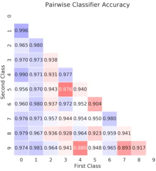
able to achieve an average test accuracy above 95%. The accuracies of the individual pairwise classifiers are tabu-lated in Fig. 9, and data from a representative example of the training process for one of the easier pairs to clas-sify is shown in 8. We observed significant differences in performance across the different pairs, partly owing, perhaps, to the difficulty of distinguishing similar digits using 64 pixel images. We also note that different choices of hyper-parameters could significantly affect which pairs were classified most accurately.

IV. IMPLEMENTATION ON NEAR-TERM

DEVICES

A key advantage of carrying out machine learning tasks with models equivalent to tree or matrix product tensor networks is that they could be implemented using a very

small number of physical qubits. The key requirement is that the hardware must allow the measurement of in-dividual physical qubits without further disturbing the state of the other qubits, a capability also required for certain approaches to quantum error correction [39]. Be-low we will first discuss how the number of qubits needed to implement either a discriminative or generative tree tensor network model can be made to scale only loga-rithmically in both the data dimension and in the bond dimension of the network. Then we will discuss the spe-cial case of matrix product state tensor networks, which can be implemented with a number of physical qubits

that is independent of the input or output data

dimen-sion.

Another key advantage of using tensor network models on near-term devices could be their robustness to noise, which will certainly be present in any near-term hard-ware. To explore the noise resilience of our models, we present a numerical experiment where we evaluate the model trained in Section III with random errors, and ob-serve whether it can still produce useful results.

A. Qubit-Efficient Tree Network Models

To discuss the minimum qubit resources needed to im-plement general tree tensor network models, recall the

notion of the virtual qubit number V from Section II.

FIG. 9. The test accuracy for each of the pairwise classifiers trained with the hyper-parameters mentioned in the text. The accuracy for each classifier can be found by choosing the po-sition along the x-axis corresponding to one class and the position on the y-axis corresponding to the other.

(8)

(a)

(b)

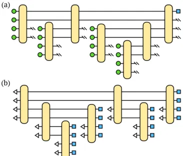
FIG. 10. Qubit-efficient scheme for evaluating (a)

discrimina-tive and (b) generadiscrimina-tive tree models withV = 2 virtual qubits

andN= 16 inputs or outputs. Note that the two patterns are

the reverse of each other. In (a) qubits indicated with hash marks are measured and the measurement results discarded. These qubits are then reset and prepared with additional in-put states. In (b) measured qubits are recorded and reset to

a reference stateh0|.

This is the number of qubit lines connecting each subtree to higher nodes in the tree. Viewed as a tensor network,

the bond dimensionD, or dimension of the internal

ten-sor indices, is given byD= 2V_.

For example, the tree shown in Fig. 7 hasV = 1 and a

bond dimension ofD= 2. The tree shown in Fig. 10 has

V = 2 andD= 4. When discussing these models in

gen-eral terms, it suffices to consider only unitary operations

acting on 2V qubits, since at each node of the tree, two

subtrees (two sets ofV qubits) are entangled together.

Given only the ability to perform state preparation

and unitary operations, it would takeN physical qubits

to evaluate a discriminative tree network model on N

inputs. However, if we also allow the step of measure-ment and resetting of certain qubits, then the number of

physical qubits Qrequired to processN inputs given V

virtual states passing between each node can be

signifi-cantly reduced to justQ(N, V) =V lg(2N/V).

To see why, consider the circuit showing the most qubit-efficient scheme for implementing the

discrimina-tive case Fig. 10(a). For a given V, the number of

in-puts that can be processed by a single unitary is 2V.

Then V of the qubits can be measured and reused, but

the other V qubits must remain entangled. So only

V new qubits must be introduced to process 2V more

inputs. From this line of reasoning and the

observa-tion that Q(2V, V) = 2V, one can deduce the result

Q(N, V) =Vlg(2N/V).

For generative tree network models, generatingN

out-(a)

(b)

FIG. 11. Qubit-efficient scheme for evaluating (a) discrim-inative and (b) generative matrix product state models for an arbitrary number of inputs or outputs. The figure shows

the case of V = 3 qubits connecting each node of the

net-work. When evaluating the discriminative model, one of the qubits is measured after each unitary is applied and the re-sult discarded; the qubit is then prepared with the next input component. To implement the generative model, one of the qubits is measured after each unitary operation and the result

recorded. The qubit is then reset to the stateh0|.

puts withV virtual qubits requires the same number of

physical qubits as for the discriminative case; this can be seen by observing that the pattern of unitaries is just the

reverse of the discriminative case for the sameN andV.

Fig. 10 shows the most qubit-efficient way to sample a

generative tree models for the case ofV = 2 virtual and

N = 16 output qubits, requiring only Q = 8 physical

qubits.

Though a linear growth of the number of physical

qubits as a function of virtual qubit number V may

seem more prohibitive compared to the logarithmic

scal-ing with N, even a small increase in V would lead to

a significantly more expressive model. From the point of view of tensor networks the expressivity of the model

is usually measured by the bond dimension D = 2V_.

In terms of the bond dimension, the number of qubits

needed thus scales only asQ(N, D)_∼lg(D) lg(N). The

largest bond dimensions used in state-of-the-art classical

tensor network calculations are aroundD= 215_{or about}

30,000. So for V = 16 or more virtual qubits one would

quickly exceed the power of any classical tensor network calculation we are aware of.

B. Qubit-Efficient Matrix Product Models

A matrix product state (MPS) tensor network is a spe-cial case of a tree tensor network that is maximally un-balanced. This gives an MPS certain advantages without sacrificing expressivity for one-dimensional distributions, as measured by the maximum entanglement entropy it can carry across bipartitions of the input or output space,

(9)

(a)

(b)

(c) (d)

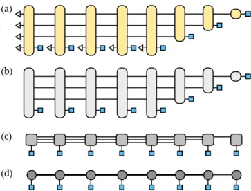
FIG. 12. Mapping of the generative matrix product state

(MPS) quantum circuit with V = 3 to a bond dimension

D= 23 MPS tensor network diagram. First (a) interpret the

circuit diagram as a tensor diagram by interpreting reference

statesh0| as vectors [1,0]; qubit lines as dimension 2 tensor

indices; and measurements as setting indices to fixed values. Then (b) contract the reference states into the unitary tensors and (c) redraw the tensors in a linear chain. Finally, (d) merge

threeD= 2 indices into a singleD= 8 dimensional index on

each bond.

Given the ability to measure and reset a subset of phys-ical qubits, a key advantage of implementing a discrim-inative or generative tensor network model based on an

MPS is that for a model withV virtual qubits, an

arbi-trary number of inputs or outputs can be processed by

using onlyV+1 physical qubits. The circuits illustrating

how this can be done are shown in Fig. 11.

The implementation of the discriminative algorithm shown in Fig. 11(a) begins by preparing and entangling

V input qubit states. One of the qubits is measured and

reset to the next input state. Then all V + 1 qubits are

entangled and a single qubit measured and re-prepared. Continuing in this way, one can process all of the inputs. Once all inputs are processed, the model output is ob-tained by sampling one or more of the physical qubits.

To implement the generative MPS algorithm shown in Fig. 11(b), one prepares all qubits to a reference state

|0i⊗V+1 and after entangling the qubits, one measures

and records a single qubit to generate the first output

value. This qubit is reset to the state _|0_i and all the

qubits are then acted on by another (V + 1) qubit

uni-tary. A single qubit is again measured to generate the second output value, and the algorithm continues until

N outputs have been generated.

To understand the equivalence of the generative circuit of Fig. 11(b) to conventional tensor diagram notation for an MPS, interpret the circuit diagram Fig. 12(a) as a ten-sor network diagram, treating elements such as reference

states _h0_| as tensors or vectors [1,0]. One can contract

or sum over the reference state indices and merge anyV

qubit indices into a single index of dimension D = 2V_.

The result is a standard MPS tensor network diagram Fig. 12(d) for the amplitude of observing a particular set of values of the measured qubits.

C. Noise Resilience

Any implementation of our proposed approach on near-term quantum hardware will have to contend with a significant level of noise due to qubit and gate imper-fections. But one intuition about noise effects in our tree models is that an error which corrupts a qubit only scrambles the information coming from the patch of in-puts belonging to the past “causal cone” of that qubit. And because the vast majority of the operations occur near the leaves of the tree, the most likely errors there-fore correspond to scrambling only small patches of the input data. We note that a good classifier should nat-urally be robust to small deformations and corruptions of the input, and, in fact, adding various kinds of noise during training is a commonly used strategy in classical machine learning. Based on these intuitions, we expect our circuits could demonstrate a high level of tolerance to noise.

In order to quantitatively understand the robustness of our proposed approach to noise on quantum hardware,

FIG. 13. The test accuracy for each of the pairwise classifiers

under noise corresponding to aT1 of 5µs, aT2 of 7µs, and

a gate time of 200 ns. In most cases, the accuracy is compa-rable to the results from training without noise. Note that it was necessary to choose a different set of hyper-parameters to enable successful training under noise.

(10)

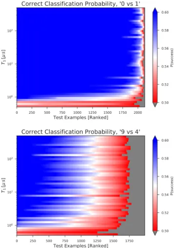
FIG. 14. Success probability of two different pairwise clas-sification circuits prediction on their test sets (sorted by

de-creasing probability of success along thex-axis) over a wide

range of T1 values (y-axis). For each T1 shown, the

proba-bility of successfully classifying each member of the test set is indicated. Note that success probabilities which are larger

than.5 even by a relatively small margin imply that the

cor-responding test example could be correctly classified with a

majority voting scheme. Gate time Tg = 200ns was held

fixed whileT2 was set to be 7₅T1. Noise levels corresponding

to current hardware are approximately two thirds of the way up the chart. Grey areas indicate regions where the model would misclassify the test example.

we study how performance is affected by independent amplitude-damping and dephasing channels applied to each qubit. In particular, we investigate how this error model would affect the pairwise tree network discrimi-native models of the type described in Section II A and shown in Fig. 7.

The specific error model we implemented is the

fol-lowing: during the contraction step of node i in the

model evaluation, we compose amplitude damping and dephasing noise channels acting on its left and right

children ρiL and ρiR, mapping ρiL → Ea(Ed(ρiL)) and

ρiR → Ea(Ed(ρiR)). Any completely positive

trace-preserving noise channel _E(ρ) can be expressed in the

operator-sum representation as E(ρ) = P

aMaρMa†,

whereP

aMaMa† =I. Here the Kraus operators Ma for

the amplitude damping channel_Ea are (in thez-basis)

M0= 1 0 0 √1−pa , M1= 0 √pa 0 0 ,

while for the dephasing channel_Edthe Kraus operators

are M0= p 1₋pdI, M1= √ pd 0 0 0 , M2= 0 0 0 √pd .

To evaluate model performance under realistic

val-ues ofpa and pd on current hardware, we determine pa

and pd based on the continuous-time Kraus operators

of these channels, which depend on the duration of the

two-qubit gateTg, the coherence timeT1 of the qubits,

and the dephasing time T2 of the qubits. Specifically,

pa = 1−e−Tg/T1 and pd = 1−e−T g/T2. Realistic

val-ues for the time scales areTg = 200 ns and T1 = 50µs,

T2= 70µs, corresponding topa= 0.004 andpd= 0.003.

But numerical experiments with these values showed al-most no observable noise effects, so we consider an even

more conservative parameter set withT1andT2reduced

by an order of magnitude, such that pa = 0.039 and

pd= 0.028.

We plot the resulting test accuracies in Fig. 13, noting that the Kraus operator formalism allows us to directly calculate the reduced density matrix of the labeling qubit under the effects of our noise model, therefore no explicit sampling of noise realizations is needed. Given that the coherence times used for the plot are easily achievable even on today’s very early hardware platforms, the re-sults shown in Fig. 13 are encouraging: many of the models give a test accuracy only slightly reduced from the noiseless case Fig. 9. The largest reduction was for the digit ‘4’ versus digit ‘9’ model, which dropped from a test accuracy of 0.88 to 0.806. Interestingly this was also the model with the worst performance in the noiseless case. The typical change in test accuracy across all of the models due to the noise was about 0.004.

To mitigate the effect of noise when classifying a par-ticular image, one can evaluate the quantum circuit some small number of times and choose the label which is most frequently observed. For example, one could take a ma-jority vote from 500 executions and classify and correctly classify an image whose individual probability of success

is.55 with almost 99% accuracy. In order to shed a more

detailed light on our approach’s robustness to noise, we plot in Fig. 14 the individual success probabilities for

classifying each test example (x-axis), sorted by their

probabilities for ease of visualization, over a range of

de-coherence times (y-axis). The two panels show two

differ-ent models, one trained to distinguish images of digits ‘0’ versus ‘1’ ; the other digits ‘9’ versus ‘4’. These models were trained and evaluated at various levels of noise us-ing the same trainus-ing hyper-parameters that were found