Improving the output of algorithms for large-scale approximate graph matching

(1)

c

(2)

IMPROVING THE OUTPUT OF ALGORITHMS FOR LARGE-SCALE APPROXIMATE GRAPH MATCHING

BY

JOSEPH LUBARS

THESIS

Submitted in partial fulfillment of the requirements

for the degree of Master of Science in Electrical and Computer Engineering in the Graduate College of the

University of Illinois at Urbana-Champaign, 2018

Urbana, Illinois Adviser:

(3)

ABSTRACT

In approximate graph matching, the goal is to find the best correspondence between the labels of two correlated graphs. Recently, the problem has been applied to social network de-anonymization, and several efficient algorithms have been proposed for approximate graph matching in that domain. These algorithms employ seeds, or matches known before running the algorithm, as a catalyst to match the remaining nodes in the graph. We adapt the ideas from these seeded algorithms to develop a computationally efficient method for improving any given correspondence between two graphs. In our analysis of our algorithm, we show a new parallel between the seeded social network de-anonymization algorithms and existing optimization-based algo-rithms. When given a partially correct correspondence between two Erdos-Renyi graphs as input, we show that our algorithm can correct all errors with high probability. Furthermore, when applied to real-world social networks, we empirically demonstrate that our algorithm can perform graph matching accurately, even without using any seed matches.

(4)

(5)

ACKNOWLEDGMENTS

Thank you to R. Srikant, my advisor, all of my instructors, my family, and friends for giving me the knowledge and support needed to make it this far. Also, thank you to Sanjay Shakkottai and Matthias Grossglauser for helpful discussions and ideas about approximate graph matching.

(6)

CHAPTER 1 INTRODUCTION

With the proliferation of publicly available social information, both released by companies and mined, privacy is becoming a large concern. Recently, after Netflix provided anonymized data to researchers on movie ratings for the Netflix Challenge, researchers were able to match the data to publicly available IMDB data to recover many identities [1]. Because of this, it is im-portant to understand how to guarantee the privacy of data which is collected or released to the public.

Social network data, such as the Facebook or LinkedIn graphs, contains rich structural information in the form of friendships or connections between users. Recently, it has become apparent that this structural information is sufficient to recover node identities, even without additional labels such as movie ratings being attached to the anonymous nodes. This process of recov-ering node identities in a partially or completely unlabeled social network is known as social network de-anonymization. In the years since Narayanan and Shmatikov demonstrated a successful de-anonymization attack on real social networks, the problem of developing efficient de-anonymization algorithms has received much scrutiny [2].

Social network de-anonymization is a recent application of a more gen-eral graph mining problem called “approximate graph matching.” The goal of approximate graph matching is to find the best correspondence between two given graphs, for some sense of “best.” This goal is a generalization of that of graph isomorphism, where an exact correspondence is required. If a graph isomorphism is found, then this isomorphism will also solve the approximate graph matching problem. In addition to network security, ap-proximate graph matching has seen various applications in many areas over

(8)

algorithm for approximate graph matching. In fact, one common setting for the approximate graph matching problem is known to be NP-hard [6]. Therefore, we turn to approximate algorithms. A broad range of approximate approaches exist for approximate graph matching, but they can be broadly divided into two categories: seedless and seeded matching algorithms.

Seedless algorithms attempt to solve the matching problem with no ad-ditional side information. Some algorithms use various relaxations of the original optimization problem. Examples include a convex relaxation ap-proach called QCV and a convex-concave apap-proach called PATH [7]. Other algorithms, such as the algorithm developed by Umeyama [8], use spectral techniques. Still other algorithms use techniques such as random walks [9] and Bayesian inference [10].

The other category of matching algorithms is the set of seeded algorithms. These require “seeds,” which take the form of a set of matches which each identify the correct correspondence for one vertex in each graph. These initial matches can be used to efficiently recover the remaining matches across the entire graph. Many seedless algorithms can be adapted to perform seeded matching, for example, by encoding the constraints into the convex program used by the QCV (convex relaxation) algorithm. Doing so can significantly improve the graph matching results [11]. However, inspired by performing de-anonymization on large-scale social networks, where some identities may not be anonymous and the network sizes can be enormous, new algorithms have been developed. The two primary algorithms are percolation graph matching, proposed by Pedarsani and Grossglauser [12], and a similar witness-based algorithm proposed by Korula and Lattanzi [13]. These and other similar algorithms have been shown to work on a fairly wide range of graph models [14].

We attempt to extend the ideas present in these seeded graph matching algorithms by asking a new question: Can we use them for correction? The output of a seedless algorithm can be interpreted as a set of seed matches, some of which are correct, and some of which are incorrect relative to an optimal solution. We develop a new algorithm, based on the algorithms in [12, 13], that will take in a partially correct graph matching and efficiently correct all of the errors. We will give a new interpretation of the matching mechanism for our algorithm, and show that it can theoretically correct all errors on a stochastic block model and, under certain assumptions, when used

(9)

as a post-processing step for other graph matching algorithms, can produce seedless graph matching with accuracy that is significantly better than the current state-of-the-art.

Our first contribution is to develop an algorithm which corrects errors in a given initial correspondence. In order to model seedless graph matching, which often produces results with some correct matches but also many un-known incorrect matches, we propose a new model where a correspondence is given between the node labels of two correlated graphs, but only a small fraction of the matches in this correspondence are correct. We show that under this model, our algorithm corrects all errors for stochastic block model graphs under certain, reasonably interpretable assumptions.

Our second contribution is to propose a general methodology for perform-ing graph matchperform-ing when there is no initial correspondence given, or only a very small number of seeds, where first an appropriate approximate graph matching algorithm is run, depending on the problem, and then our algorithm is run on the output. Using extensive numerical experiments on both random graph models (including models other than the stochastic block model) and real social network datasets, we show that using our algorithm as a post-processing step improves the results produced by state-of-the-art algorithms for approximate graph matching.

The rest of the thesis is organized as follows. Chapter 2 contains our mathematical model and problem statement. Chapters 3 and 4 contain our main result and its proof, respectively. Chapter 5 relates our work to prior work on the problem. Chapter 6 contains simulation results, and concluding remarks are presented in Chapter 7.

(10)

CHAPTER 2 MODEL AND PROBLEM STATEMENT

In order to generate two correlated graphs G1 and G2, we use the following

subsampling model. We start with an underlying graph G = (V, E) on n nodes, which can be interpreted, for example, as the set of all acquaintances among n people. Each edge of G is sampled independently with probability s for inclusion into a subgraph G1, which could represent the relationships

present between the individuals in one social network. Independently, the edges are sampled again with probability s to produce another graph G2,

which could represent the relationships between the same individuals in a different social network. However, the identities of the individuals in G2 are

anonymized, or unknown. Therefore, we permute the vertices ofG2according

to a permutation π, chosen uniformly at random. Given G1 = (V1, E1) and

π(G2) = (V2,E˜2), the goal is to recover π. This model was introduced by

Pedarsani and Grossglauser in the case thatG is an Erd¨os-R´enyi graph [15]. However, here, we will assume a more general stochastic block model for G: Partition V into k communities: V = C1 tC2 t. . .tCk. Then, given a

symmetric k×k matrix P of community connection probabilities, connect vertices between communitiesCiandCj with probabilityPij. We will assume

thatPii ≥Pij for alli, j, so edges are more likely within the same community.

Various algorithms exist for solving this approximate graph matching prob-lem. However, they are, in general, imperfect, and may only successfully recover π(v) for a subset of the vertices v in V. We wish to start with an estimate ˆπ which agrees with π on an unknown subset of V, and then use this estimate to correct these unknown errors and recover π exactly with high probability. In our model, we assume the initial estimate ˆπ is randomly generated with a constant fraction β of correct matches as follows:

First, a subset W ⊂ V is generated by sampling each vertex in V with probability β. For each v ∈ W, set ˆπ(v) = π(v). Next, generate a per-mutation πW of V \ W uniformly at random. For each v ∈ V \ W, set

(11)

ˆ

π(v) = π(πW(V)). Our algorithm is intended as a post-processing step for

other algorithms which may produce such a ˆπ. However, it is difficult to model exactly how such algorithms will produce their estimate ˆπ. Our mod-eling assumption on ˆπis used to obtain tractable theoretical results. However, the algorithm we obtain works remarkably well in practice, even though the pre-processing algorithms may or may not produce an estimate that agrees with our assumptions.

(12)

CHAPTER 3 MAIN RESULTS

3.1 Basic Algorithm

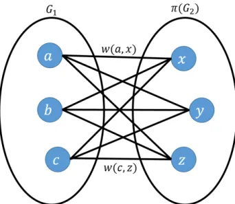
To correct the errors of ˆπ, we propose an algorithm based on “witnesses,” as defined in [13]: for each pair (v1, v2), where v1, v2 ∈ V, we count the

number of witnesses for that pair, defined as the set of vertices x such that (v1, x)∈ E1 and (v2,π(x))ˆ ∈E˜2. Let w(v1, v2) be this number of witnesses.

Each of these witnesses encodes some evidence that π(v1) = v2. Therefore,

we would like to find a maximum weight bipartite matching using the weights w(v1, v2) in order to improve our estimate of ˆπ(see Figure 3.1). The complete

algorithm is presented as Algorithm 1 below. Algorithm 1: Basic Correction Algorithm

Input: G1, π(G2), ˆπ

InitializeW = zeros(n×n) for u in V do

for v in V do

Calculate Wu,v =w(u, v)

Return MaximumWeightMatching(W)

Unfortunately, for large values of n, this procedure is inefficient. Naively iteratively computing w(u, v) for every u and v requires at least n2 com-putations, which is infeasible for large social networks which may contain thousands or even millions of nodes. Similarly, maximum weighted bipartite matching can be done in n(|W|+nlog(n)) time, where |W| is the number of nonzero entries of W [16]. This is also too inefficient for large values of n. Instead, we will replace the procedure for constructing W by a more ef-ficient procedure featuring the “CountPaths” subroutine, introduced below, which can achieve a better complexity of O(|E1|∆2), where ∆2 is the largest

(13)

Figure 3.1: Maximizing the number of witnesses as a bipartite matching problem

degree of a vertex in G2. In an Erd¨os-R´enyi graph with p = O(log(n)/n),

for example, at the threshold for connectivity, our this procedure runs in O(nlog2(n)) time. We will also replace the maximum weight matching by a greedy matching (complexity |W|log(|W|)). In practice, and theoretically in the case of the stochastic block model, the greedy matching is sufficient to recover π perfectly from ˆπ.

Algorithm 2: Optimized Correction Algorithm Input: G1, π(G2), ˆπ

for u in V do

W(u,·) = CountPaths(G1, π(G2), ˆπ,u)

Return GreedyMaximumWeightMatching(W)

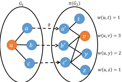
CountPaths relies on the interpretation that every vertex x which is a witness for (u, v) can be thought of as a “path” from u, to a, to π(a), to v, where the first edge (u, a) is an edge in G1, the second edge (a, π(a)) is along

the mapping π, and the third edge (π(a), v) is an edge in π(G2) (see Figure

3.2). Counting these paths can be implemented as a simple iterative process, reproduced below.

(14)

Figure 3.2: Counting paths to determine witnesses for (u, v) Algorithm 3: CountPaths Input: G1, π(G2), ˆπ,u InitializeW(u,·) = 0 for x∈G1.neighbors(u) do for v ∈π(G2).neighbors(ˆπ(x))do W(u, v) += 1 ReturnW(u,·)

(15)

3.2 Iterated Algorithm

One feature of our matching algorithm is its ability to take a mapping as input and output an improved mapping. It is then natural to take the new, improved mapping and feed it back into our algorithm, to further improve it. This is the intuition behind the iterated correction algorithm, presented as Algorithm 4:

Algorithm 4: Iterated Correction Algorithm Input: G1, π(G2), ˆπ,k

for iteration = 1, . . . , k do ˆ

π=OptimizedCorrection(G1, π(G2),π)ˆ

Return ˆπ

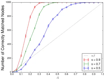
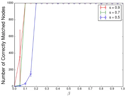
As long as the first iteration of our algorithm is able to improve the ac-curacy of the original input matching, further iterations should be able to further improve, until a local optimum is reached, where (hopefully) all nodes are matched correctly. An illustration of this phenomenon is available in Fig-ures 3.3 and 3.4. As long as one iteration of our algorithm performs above the dotted line (corresponding to producing more correct matches than in the input matching), then the iterated algorithm is able to correct all errors in the input matching.

3.3 Intuition

One metric sometimes used for quantifying the correctness of an approximate graph matching is the “overlap metric,” which counts the number of edges on which two graphs G1 = (V, E1) and G2 = (V, E2) agree. The larger

this metric, the more evidence we have that G1 and G2 are the same. In

our setting where G1 and G2 are random objects, this can be conveniently

expressed using indicator variables _I: ∆(G1, G2) =

XX

(16)

Figure 3.3: Erd¨os-R´enyi graphs for varying values ofβ. Algorithm 2 is used.

(17)

mutations, attempting to recover π: max π0 X u∈V X v∈V I{(u, v)∈E1,(π0(u), π0(v))∈E˜2} (3.2)

This natural approach is the maximum likelihood estimator in the case that G is an Erd¨os-R´enyi graph and G1 and G2 are sampled according to

our model [17]. However, it is very difficult to solve exactly. Our approach, given an estimate matching ˆπ, is to solve the maximization problem using our estimate in place of π0 in one spot:

max π0 X u∈V X v∈V I{(u, v)∈E1,(π0(u),π(v))ˆ ∈E˜2} (3.3)

Note that the inside sum is merely the number of witnesses for u and π0(u): max

π0

X

u∈V1

w(u, π0(u)) (3.4)

This one change transforms the problem from an extremely difficult combi-natorial optimization problem into a much simpler maximum weighted bipar-tite matching problem, which can now be solved efficiently. The assumption is that if ˆπ is close enough to π, the solutions to (3.2) and (3.3) will also be close.

In order to provide intuition as to why this is true, we will consider the simple case where G is an Erd¨os-R´enyi graph with edge probability p. Pro-ceeding in a similar manner to Yartseva and Grossglauser in [12], look at the indicator _I{(u, v) ∈ E1,(ˆπ(u), π0(v)) ∈ E˜2} in (3.3). Suppose ˆπ(v) = π(v).

Then if π0(u) = π(u), it takes the value 1 if (u, v) ∈ E and the edge is sampled twice, for a total probability of ps2_{. However, in any other case,}

(u, v) in E1 and ( ˆπ(u), π0(v)) in E2 no longer are sampled from the same

edge in the underlying graph E. Therefore, the indicator takes the value 1 with probability only p2s2. Because pis assumed to be small, p2s2 << ps2.

We expect approximately n(βps2 _{+ (1}₋ _β)p2_s2_{) witnesses for a correct}

match (u, π(u)), and only approximately np2_s2 _{witnesses for an incorrect}

(18)

Figure 3.5: w(u, v) foru, v ∈G1, G2. Here, G is Erd¨os-R´enyi(40, 0.25),

s = 0.9, and ˆπ agrees with π=identity on 20 vertices. argument formal for the stochastic block model below.

3.4 Connection to Optimization-Based Methods

There is another way to represent the witness matrixW which is enlightening. Letting A1 be the adjacency matrix of G1 and A2 the adjacency matrix of

π(G2), we note thatw(u, v) is the inner product of theu-th row ofA1 and the

ˆ

π(v)-th row of A2. Therefore, if ˆP is the permutation matrix corresponding

to ˆπ, we can express W succinctly as:

W =AT₁P Aˆ 2 (3.5)

One way to write the overlap metric in matrix form (defined in the previous section) is as follows:

f( ˆP) = ∆(G1,π(Gˆ 2)) = T r( ˆP AT1Pˆ

T_A

(19)

It is easy to verify that, in fact, our witness matrix W is proportional to the gradient of f:

∇f( ˆP) =AT₁P Aˆ 2+A1P Aˆ T2 = 2A

T

1P Aˆ 2 (3.7)

This implies a connection between witness-based methods like ours and optimization-based methods based on the overlap metric. The closest con-nection is to the Frank-Wolfe algorithm. Following is the Frank-Wolfe algo-rithm for maximizing f over the set of doubly stochastic matrices (Πn here

is the set of n×n permutation matrices):

Algorithm 5: Frank-Wolfe Algorithm for Approximate Graph Match-ing

Input: Initial Guess P0, A1, A2, k

for i= 0, . . . , k−1 do Compute W = 2A1PiTA2

Use the Hungarian algorithm to maximize hQ, Wisubject to Q∈Πn

Maximize h((1−γ)Pi+γQi)TA1((1−γ)Pi+γQi), A2i over

γ ∈[0,1]

Set Pi+1 ⇐Pi+γ(Q−Pi)

Find ˆP to maximizehPk, PiforP ∈Π using the Hungarian Algorithm

For comparison, following is our iterated algorithm:

Algorithm 6: Our Iterated Correction Algorithm (Again) Input: Initial Guess P0, A1, A2, k

for i= 0, . . . , k−1 do Compute W =A1PiTA2

Use the greedy matching to approximately maximize hQ, Wi subject toQ∈Πn

γ = 1

Set Pi+1 ⇐Pi+γ(Q−Pi)

ReturnPk

The only difference here is that we are approximately solving the linear assignment problem to compute Q, and we are always using a step size γ

(20)

matrix at every step, ensuring that computing W always remains efficient. In practice, it seems to work well, often still converging to a good solution.

3.5 Performance Guarantees

Givenn,P,C1, . . . , Ck, andβ, letG,G1,G2,π, and ˆπbe generated according

to our model above (so G is generated from a stochastic block model). We define di as follows for each community i ∈[k], with the interpretation that

di is the average degree in G for vertices in community i:

di :=Pii(|Ci| −1) + X

j∈[k]\{i}

Pij|Cj| (3.8)

Then, as long as the minimum di is large enough, but not so large as to

make the graph too densely connected, the optimized correction algorithm above will perfectly recover π with high probability (in the asymptotic limit as n increases):

Theorem 1 Suppose s2βmini∈[k]di > 16 log(n) and Pij = o(1) for all i, j.

Then the optimized correction algorithm recovers π from πˆ with probability

1−o(1).

As a corollary, by setting every entry of P to be equal top, we recover a result similar to that of Korula and Lattanzi [13]:

Corollary 1 SupposeGis Erd¨os-R´enyi(n, p), where (n−1)ps2_{β >}_{16 log(n)}

andp=o(1). Then the optimized correction algorithm recoversπfromπˆwith probability 1−o(1).

These results can be interpreted as follows: First, the expected degree of every node should be high enough that the intersection of G1 and G2 is

con-nected. For Erd¨os-R´enyi graphs, it is known that if nps2 <log(n), then no algorithm can recover π, given no side information, and if nps2 > 2 log(n), then the maximum likelihood estimator succeeds with high probability [17]. Our lower bound on the average degree is therefore within a constant factor

(21)

of optimal for Erd¨os-R´enyi graphs. Secondly, the graphs should not be too densely connected. Some limit on the density of the graphs is required, as matching two graphs is equivalent to matching their complements, and we have already established that the graphs cannot be too sparse. Furthermore, most real-life networks have relatively small degrees or even constant aver-age degrees, so forcing the degree of each node to be o(n) is a reasonable assumption in this light.

Interestingly, none of our proofs depend on the number of communitiesk. Therefore, we can let k grow with n as fast as we like, or even set k =n to independently designate each edge probability in our graph G. This allows us to extend our result to other models utilizing independent Bernoulli edges such as the Chung-Lu model (see [18]), as long as the expected degree di of

each node is large enough to satisfy the same constraint s2_βd

i >16 log(n):

Corollary 2 Let P be a symmetricn×n matrix, and let G= (V, E) be the undirected graph with each edge (i, j) independently present with probability

Pij. Suppose Pij =o(1)for alli, j. Furthermore, assume that for every vertex

i, the expected degree di satisfies s2βdi > 16 log(n). Then, the optimized

(22)

CHAPTER 4 PROOF

The general strategy will be to show that with high probability, w(u, π(u))> w(u, v) for all u and all v 6= u. Then, a greedy maximum weight matching will match u with π(u) for each u. In order to show that w(u, π(u)) domi-nates other numbers of witnesses for a given w, we will show the following results:

Lemma 1 For each u∈V, suppose u∈Ci. Then, if s2βdi >16 log(n):

P w(u, π(u))< 3 8s 2_βd i =O(n−32) (4.1)

Lemma 2 For each u ∈ V and v ∈ V \ {π(u)}, suppose u ∈ Ci. Then, if

s2_βd

i >16 log(n) and Pjj =o(1) for every j:

P w(u, v)> 3 8s 2_βd i =O(n−4) (4.2)

Lemma 1 says that the number of witnesses obtained for a correct match is at least a constant times the average number of witnesses expected from cor-rect matches. Independently, we also show with Lemma 2 that no incorcor-rect match ever reaches this same number of witnesses. By the union bound, these thresholds are respected with high probability for every u and v. Therefore, w(u, π(u)) > w(u, v) for all u and for all v 6= u. By the reasoning given at the beginning of the section, therefore the theorem is proved.

To show the second corollary, note that the graph generation process is equivalent to the stochastic block model with n communities. Setting the diagonal entries of P to be equal to the maximum of their rows gives us the condition Pjj = o(1) for every j. Therefore, Lemma 1 and 2 still apply to

(23)

4.1 Proofs of Lemmas

In order to prove lemmas 2 and 3, it will be convenient to express w(u, v) as a sum of indicators as follows:

X

x∈V1\{u}

I{(u, x)∈E1,(v,π(x))ˆ ∈E˜2} (4.3)

We will also find the following two Chernoff bounds useful (see, for exam-ple, [19]):

Bound 1 If X = X1 +. . .+Xn, where the {Xi} are independent random

variables taking values in {0,1}, then for δ∈(0,1) we have:

P(X <(1−δ)E[X])≤exp(−δ

2

E[X]

2 ) (4.4)

Bound 2 If X = X1 +. . .+Xn, where the {Xi} are independent random

variables taking values in {0,1}, then for δ >1 we have:

P(X >(1 +δ)E[X])≤exp(−δE[X]

3 ) (4.5)

4.1.1 Proof of Lemma 1

Recall that in our generation of ˆπ, first every vertex is sampled with proba-bility β to form a subset W ⊂ V, and those vertices are matched correctly in ˆπ. Let A(u, x) be the indicator that (u, x) ∈ E1, (π(u), π(x)) ∈ E2, and

x∈W. Clearly, we have:

w(u, π(u))≥ X

x∈(F1∪...∪Fk)\{u}

A(u, x)

After fixing u, each A(u, x) is independent for all x 6= u. The indicators all take the value 1 with probability βPijs2, for appropriate Pij. Therefore:



X



(24)

P w(u, π(u))< 1 2s 2 βdi ≤exp(−s 2_βd i 8 ) ≤exp(−2 log(n)) = 1 n2

where we used the assumption that s2_βd

i ≥16 log(n).

4.1.2 Proof of Lemma 2

For this proof, assume the following procedure is used to produceG= (V, E): First, create an Erd¨os-R´enyi graph GER = (V, EER) with edge probability

pmax := maxjPjj. Then, independently, for every edge (u, v) ∈ EER with

u ∈ Ci and v ∈ Cj, sample the edge (u, v) with probability Pij/(pmax) to

obtain E. Clearly, this process is stochastically identical to the original creation process for the stochastic block model.

For this proof, we always assume v 6=π(u) and u ∈ Ci. For now, choose

an arbitrary fixed ˆπ. This time, we decompose the sum (4.3) as w(u, v) = X j∈[k] X x∈Cj\{u} I n (u, x)∈E1,(v,π(x))ˆ ∈E˜2 o

The indicator in the summand above can be stochastically dominated by an indicator (denoted by B(u, v, x)) for the following event: (u, x) ∈ E, (v,π(x))ˆ ∈ EER, (u, x) is sampled for inclusion into E1 (with probability

s), and (v,π(x)) is sampled for inclusion into ˜ˆ E2 (with probability s). This

indicator B(u, v, x) is independent for every x 6=u, is 0 if ˆπ(x) = v, and is Ber(s2_P

ij(pmax)), otherwise, where x ∈ Cj. We will bound the case when

B(u, v, x) = 0 by a Bernoulli random variable as well. We can therefore bound the sum, conditioned on our choice of ˆπ:

P w(u, v)>(1 +δ)s2(pmax)di <exp(−δs 2_(p max)di 3 )

Letting 1 +δ= (3β)/(8(pmax)), we get for large enough n:

P w(u, v)> 3 8βs 2_d i <exp −( 3β 8(pmax) −1)s 2_(p max)di 3 !

(25)

But (₈₍_p3β

max) −1)(pmax) < β, so combining that with s

2_βd

i > 16 log(n)

gives us the result conditioned on ˆπ. However, since the bound holds for every choice of ˆπ, it also holds without conditioning on ˆπ, and the result is proved.

(26)

CHAPTER 5 RELATIONSHIP TO PRIOR WORK

Our algorithm for approximate graph matching correction uses the concept of witnesses presented by Korula and Lattanzi in [13]. This paper first presents the idea of counting witnesses, and we use similar terminology. However, in their theoretical analysis, the seed set is assumed to be accurate. This also precludes the case where the seed set encompasses the entire graph. When these assumptions are relaxed, we showed that the algorithm can then be viewed as a sort of bipartite matching problem. Their degree bucketing approach can be viewed as a sort of greedy matching algorithm in that light. Furthermore, we give the first analysis of a witness method with highly noisy seeds.

Noisy seeds have been considered in the past for similar algorithms by Kazemi, Hassani, and Grossglauser [20]. Here, however, the algorithm that is analyzed, when modified for our use case, does not perform well on gen-eral graph models, due to the thresholding that they use for the percolation model. Their more applicable algorithm is heuristic in nature and cannot be applied directly to graph matching correction. Furthermore, unlike other papers covering similar graph matching approaches, we apply our analysis to the stochastic block model [21, 12, 14].

(27)

CHAPTER 6 SIMULATION RESULTS

We examine the performance of our graph matching correction algorithm, and present experiments to attempt to answer the following questions:

1. How does our algorithm perform on our model?

2. How does our algorithm perform for correcting seedless graph match-ing?

3. How does our algorithm perform for correcting with a small number of seeds?

6.1 Results for Subsampling Model

Recall that in our subsampling model, there is an initial graph G, whose edges are sampled twice with probability s to create two correlated graphs to match. Then, we are given a permutation ˆπ to correct, which matches the two graphs correctly on a fraction β of vertices. We apply this model to a number of graphs G, both synthetic and real-world, and evaluate the performance of our correction algorithm.

6.1.1 Synthetic Graphs

For our first experiment, we attempt to use our algorithm to correct match-ing errors, assummatch-ing a ˆπ randomly generated according to our model and assuming that G is an Erd¨os-R´enyi graph withn = 1000 and (n−1)p= 40, randomly generated and sampled according to various values of s for each

(28)

Figure 6.1: Stochastic block model graphs for varying values of β. Iterated algorithm used.

the graph is 40, and P11 =P22 = 2P12. The performance, plotted in Figure

6.1, is similar to that of the Erdös-Rényi graph. Finally, we run our algorithm on Barabási-Albert graphs, a more realistic model for social networks, again chosen with an average degree of 40. The performance is similar, as shown in Figure 6.2. Note that when s= 0.5, some nodes are isolated in either G1

or G2 and therefore cannot be matched at all by our algorithm.

6.1.2 Real-World Graphs

All of the graphs used so far have been synthetic, but our algorithm also per-forms well when the subsampling model is applied to real-world graphs. For this experiment, we used a snapshot of the Slashdot social network (Figure 6.3) and a snapshot of the Epinions social network (Figure 6.4) with 77360 and 75888 nodes, respectively [22]. We sampled each edge twice with proba-bilities 0.5, 0.7, and 0.9, and evaluated the performance of our algorithm on our model, for various values of β.

Interestingly, for s = 0.9, our algorithm could sometimes match a large fraction of nodes with no seed information, making it an efficient seedless graph matching algorithm. Again, large fractions of nodes were isolated in

(29)

Figure 6.2: Barab´asi-Albert graphs for varying values of β. Iterated algorithm used.

(30)

Figure 6.4: Error correction on the Epinions social network graph for varying values of β. Iterated algorithm used.

eitherG1orG2after edge sampling, making those nodes impossible to match

using our algorithm.

6.1.3 Beyond the Subsampling Model

Naturally, real-world examples of G1 and G2 may not be generated by

sam-pling edges independently from a ground-truth graph G. To show that our algorithm works even in this case, we examine the two-hop neighborhood of the article for “Earth” in both the French and German Wikipedia, as they appeared on June 20, 2017. Wikipedia maintains inter-language links, which we use as the canonical correspondence between the two graphs. We treat links between different articles as undirected edges in the graphs. For this experiment, we let G1 and G2 be the subgraph in each respective

lan-guage containing articles which are present in both two-hop neighborhoods of “Earth.” The results can be found in Figure 6.5.

We note that in many real-life graphs, it may be impossible to match all of the nodes. Generally, if there exists an automorphism (i.e., a permutation of the nodes that leaves the adjacency graph unchanged) of either G1 orG2

(31)

Figure 6.5: Error correction on a subgraph of the French and German Wikipedia graphs (containing 8418 articles), for varying values of β. Iterated algorithm used.

uniquely determined. For example, there could be multiple isolated nodes, or multiple degree-1 nodes with the same neighbor. In the French and German Wikipedia subgraphs, each subgraph has 8418 nodes, but we can only recover approximately 3260 of the correct correspondences. We examined one ˆπ obtained for β = 0.1, and verified that it is correct up to an automorphism of G1 and G2, so we succeeded in correctly identifying all correspondences

between the two graphs which were possible to discern uniquely.

6.2 Seedless Graph Matching

One primary application of our algorithm is in correction of seedless graph matching algorithms. Such algorithms include QCV [7], PATH [7], and a Bayesian approach [10]. We test the performance of our algorithm in correct-ing initial matchcorrect-ings made by each of these algorithms on Barab´asi-Albert graphs. For these experiments, we use n= 500, as some of these algorithms

(32)

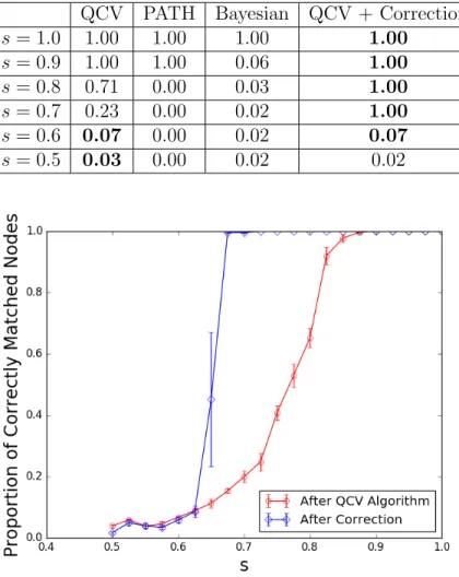
Table 6.1: Average precision after various seedless matching techniques QCV PATH Bayesian QCV + Correction

s= 1.0 1.00 1.00 1.00 1.00 s= 0.9 1.00 1.00 0.06 1.00 s= 0.8 0.71 0.00 0.03 1.00 s= 0.7 0.23 0.00 0.02 1.00 s= 0.6 0.07 0.00 0.02 0.07 s= 0.5 0.03 0.00 0.02 0.02

Figure 6.6: Error correction on the QCV algorithm using our algorithm and PATH, we use the implementation from the publicly available GraphM package [7]. For the Bayesian method developed by Pedarsani et al., we use the implementation provided by SecGraph [10, 23].

Although the performance degrades rapidly for all of the seedless algo-rithms as s decreases, QCV still manages to match a fraction of nodes cor-rectly, allowing our algorithm to correct the remaining errors and outperform every seedless algorithm run in isolation. Figure 6.6 shows this phenomenon for QCV on various values of s.

(33)

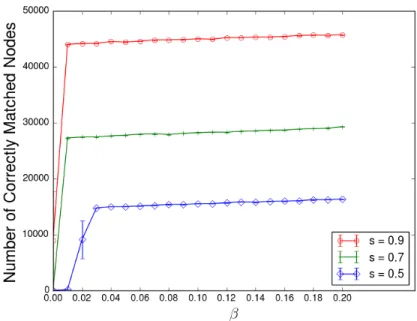
Figure 6.7: Number of correctly matched nodes on the Epinions graph (sampled with s = 0.9), after ExpandWhenStuck from [20] and after correction

6.3 Graph Matching with a Small Number of Seeds

In addition to seedless graph matching algorithms, we can boost the perfor-mance of some seeded algorithms. In [20], Kazemi and Grossglauser present an algorithm called ExpandWhenStuck that can perform approximate graph matching on very large graphs with just a handful of seeds. Their algorithm matches a large fraction of nodes correctly on the Epinions social networks when starting with even just one seed. However, with such a small number of seeds, the accuracy of the matching suffers. We apply our algorithm as a post-processing step, and universally improve the results when starting with ten or fewer seeds, as seen in Figure 6.7. For a fair comparison, we have restricted ourselves to matching only nodes with two or more witnesses for this experiment, as ExpandWhenStuck uses a similar technique to increase precision.

(34)

CHAPTER 7 CONCLUSIONS

Approximate graph matching is a hard problem in general, but efficient al-gorithms exist to solve the problem on a wide range of graphs, in practice. Sometimes, these algorithms produce sub-optimal results. However, using ideas learned from seeded graph matching algorithms, we can improve these results to produce state-of-the-art graph matching results.

Although we have only proven that our algorithm can correct a random initial distribution of errors on stochastic block model graphs, in practice, the effect seems much more general. We suspect there is a general thresh-olding effect: if enough initial seeds are present, all correct matches can be recovered, regardless of the initial condition, but if not enough are present, then no matches can be recovered. This implies that the greatest difficulty for approximate graph matching is to match just a few vertices. Quantifying this difficulty is an interesting direction for future research.

(35)

REFERENCES

[1] A. Narayanan and V. Shmatikov, “Robust de-anonymization of large sparse datasets,” in Security and Privacy, 2008. SP 2008. IEEE Sym-posium on. IEEE, 2008, pp. 111–125.

[2] A. Narayanan and V. Shmatikov, “De-anonymizing social networks,” in

Security and Privacy, 2009 30th IEEE Symposium on. IEEE, 2009, pp. 173–187.

[3] A. Toshev, J. Shi, and K. Daniilidis, “Image matching via saliency region correspondences,” in Computer Vision and Pattern Recognition, 2007. CVPR’07. IEEE Conference on. IEEE, 2007, pp. 1–8.

[4] G. W. Klau, “A new graph-based method for pairwise global network alignment,” BMC Bioinformatics, vol. 10, no. 1, p. S59, 2009.

[5] E. Kazemi, H. Hassani, M. Grossglauser, and H. P. Modarres, “Proper: Global protein interaction network alignment through percolation matching,” BMC Bioinformatics, vol. 17, no. 1, p. 527, 2016.

[6] J. W. Raymond and P. Willett, “Maximum common subgraph isomor-phism algorithms for the matching of chemical structures,” Journal of Computer-Aided Molecular Design, vol. 16, no. 7, pp. 521–533, 2002. [7] M. Zaslavskiy, F. Bach, and J.-P. Vert, “A path following algorithm for

the graph matching problem,” IEEE Transactions on Pattern Analysis and Machine Intelligence, vol. 31, no. 12, pp. 2227–2242, 2009.

[8] S. Umeyama, “An eigendecomposition approach to weighted graph matching problems,” IEEE Transactions on Pattern Analysis and Ma-chine Intelligence, vol. 10, no. 5, pp. 695–703, 1988.

[9] M. Gori, M. Maggini, and L. Sarti, “Exact and approximate graph matching using random walks,” IEEE Transactions on Pattern Anal-ysis and Machine Intelligence, vol. 27, no. 7, pp. 1100–1111, 2005.

(36)

[11] V. Lyzinski, D. E. Fishkind, and C. E. Priebe, “Seeded graph match-ing for correlated Erd¨os-R´enyi graphs.” Journal of Machine Learning Research, vol. 15, no. 1, pp. 3513–3540, 2014.

[12] L. Yartseva and M. Grossglauser, “On the performance of percolation graph matching,” in Proceedings of the first ACM conference on Online social networks. ACM, 2013, pp. 119–130.

[13] N. Korula and S. Lattanzi, “An efficient reconciliation algorithm for social networks,” Proceedings of the VLDB Endowment, vol. 7, no. 5, pp. 377–388, 2014.

[14] C. Fabiana, M. Garetto, and E. Leonardi, “De-anonymizing scale-free social networks by percolation graph matching,” in Computer Commu-nications (INFOCOM), 2015 IEEE Conference on. IEEE, 2015, pp. 1571–1579.

[15] P. Pedarsani and M. Grossglauser, “On the privacy of anonymized net-works,” in Proceedings of the 17th ACM SIGKDD International Con-ference on Knowledge Discovery and Data Mining. ACM, 2011, pp. 1235–1243.

[16] M. L. Fredman and R. E. Tarjan, “Fibonacci heaps and their uses in im-proved network optimization algorithms,”Journal of the ACM (JACM), vol. 34, no. 3, pp. 596–615, 1987.

[17] D. Cullina and N. Kiyavash, “Improved achievability and converse bounds for Erd¨os-R´enyi graph matching,” in Proceedings of the 2016 ACM SIGMETRICS International Conference on Measurement and Modeling of Computer Science. ACM, 2016, pp. 63–72.

[18] W. Aiello, F. Chung, and L. Lu, “A random graph model for massive graphs,” in Proceedings of the Thirty-Second Annual ACM Symposium on Theory of Computing. Acm, 2000, pp. 171–180.

[19] D. P. Dubhashi and A. Panconesi, Concentration of Measure for the Analysis of Randomized Algorithms. Cambridge University Press, 2009. [20] E. Kazemi, S. H. Hassani, and M. Grossglauser, “Growing a graph matching from a handful of seeds,” Proceedings of the VLDB Endow-ment, vol. 8, no. 10, pp. 1010–1021, 2015.

[21] C.-F. Chiasserini, M. Garetto, and E. Leonardi, “Impact of clustering on the performance of network de-anonymization,” in Proceedings of the 2015 ACM on Conference on Online Social Networks. ACM, 2015, pp. 83–94.

(37)

[22] J. Leskovec and A. Krevl, “SNAP Datasets: Stanford large network dataset collection,” http://snap.stanford.edu/data, June 2014.

[23] S. Ji, W. Li, P. Mittal, X. Hu, and R. A. Beyah, “Secgraph: A uniform and open-source evaluation system for graph data anonymization and de-anonymization,” inUSENIX Security Symposium, 2015, pp. 303–318.