Health Insurance Estimates for Counties1 Robin Fisher and Joanna Turner
U.S. Census Bureau, HHES-SAEB, FB 3 Room 1462
Washington, DC, 20233 Phone: (301) 763-3193, email: robin.c.fisher@census.gov
1 This paper reports the results of research and analysis undertaken by the U.S. Census Bureau staff. It has undergone a Census Bureau review more limited in scope than that given to official Census Bureau publications. This report is released to inform interested parties of ongoing research and to encourage Key Words: Small Area Estimates; Health
Insurance Coverage; ASEC 1. Introduction
There is broad public interest in health insurance coverage issues. The number of uninsured people in the United States increased by roughly 10 million in the 1990s, despite a strengthening economy (Mills, 2002). With the failure of the proposal for universal health insurance coverage in the mid 1990s, it became apparent that targeted policies would be the path to follow for programs designed to increase coverage in the population. In order to determine how one would best target certain populations that may have disproportionate levels of non-coverage, policy makers need to be able to accurately identify these groups. The U.S. Census Bureau Small Area Health Insurance Estimates (SAHIE) project of the Small Area Estimates Branch (SAEB) is researching the feasibility of producing model-based estimates of the number of people not covered by health insurance (i.e. uninsured) for states and counties.
Generally, health insurance coverage statistics are available only through national household surveys, and the estimates from these surveys vary widely for a number of well-documented reasons (Lewis et al, 1998). The Annual Social and Economic Supplement (ASEC) to the Current Population Survey (CPS) is the most widely cited source for health insurance statistics. It is annual, the data are released in a timely manner, the sample size is relatively large, and it has a state-based design. Sample sizes are not large enough, however, that the survey alone can produce sufficiently reliable
state estimates for many policy purposes. While recent follow-up legislation has provided the U.S. Census Bureau with additional funding in order to improve these estimates, reliance on surveys alone will continue to prevent the use of direct estimators for sub-state levels of geography.
Recent methodological developments, at both the U.S. Census Bureau and in the broader research community, offer new potential for developing estimates of various uninsured populations in small areas. SAEB has played a significant role in this field, developing a program that produces income and poverty estimates at the state, county, and school district levels. The Small Area Income and Poverty Estimates (SAIPE) program constructs statistical models that relate income and poverty to various indicators based on the following data:
• Federal tax returns • Food stamp participation
• Estimates from the Bureau of Economic Analysis
• Estimates from the Social Security Administration
• Estimates from the U.S. Census Bureau’s Population Division • Decennial census.
These are then combined with direct estimates from the ASEC to provide estimates and standard errors for the geographic areas of interest. The SAIPE estimates were evaluated favorably by the Panel on Estimates of Poverty for Small Geographic Areas of the National Academy of Sciences (National Research Council, 2000). They are used in Title I funding allocation formulas of the No Child Left Behind Act of 2001 by the Department of Education, and
by the Department of Health and Human Services to gauge the efficacy of welfare reform programs on children.
This paper is part of an ongoing effort to expand SAIPE knowledge and methodologies to the area of health insurance coverage. The effort began with Fisher and Campbell (2002), who modeled the numbers of children of interest for the State Children’s Health Insurance Program (SCHIP). This paper uses a Bayesian version of the method used in the SAIPE poverty models, with some modifications, to estimate the insurance coverage rate at the county level, from which the number of uninsured can be calculated. The paper proceeds as follows: Section 2 describes our data sources; Section 3 describes the model; Section 4 discusses the estimation; preliminary results are provided in Section 5; we conclude and describe future plans in Section 6.
2. Data
We describe the variables we considered, although not all were included in the model. a. CPS
•
Log proportion insured. This is the log of the ratio of the total insured to the population, measured by the ASEC; this is a three-year average of the three ASEC direct estimates, centered on the year of interest, weighted by the number of households in sample. The ASEC sample is reweighted so each county’s direct estimate is approximately unbiased for the number of insured for that county. This is denoted LINSHRifor county i. Note that, for every county with sample, there are insured people. Thus when the log proportion insured is calculated, there are no counties for which the response is undefined. There are 1198 counties with sample in at least one of the three years, with an average of 123 households in sample.
b. Internal Revenue Service (IRS)
This is information from individual tax returns aggregated by the U. S. Census Bureau to state and county levels using the street address on the return. The total number of exemptions attributed to a return includes the filer, the
spouse of the filer, and the number of child exemptions for the household. For more details see
http://www.census.gov/hhes/www/saipe/techdoc/ inputs/taxdata.html.
• Log IRS proportion between multiples of the Federal Poverty Threshold (FPT). This is the log of the fraction of exemptions on tax returns living in households with money income between two proportions of the FPT, say p1 and p2. This is denoted lpoorini(p1, p2) for county i. Available
values for pk are 0%, 50%, 100%, 130%, 200%, 300%, and infinity. Of particular interest is lpoorini(100%,
130%); these are low income people for whom the expense of health insurance may be too high and who may not be covered by a program that targets the uninsured poor. An alternative summary to the proportions between multiples of the FPT follows.
• IRS moment of the log ratios of individuals’ family income to their Federal Poverty Threshold (FPT). This is , ln ) ( r N j ij ij i j FPT inc r LIPR
∑
= r =1, . . . , 4. FPTij is the FederalPoverty Threshold for the family of person j in county i. Family money income of that person is incij. These
moments contain information about the shape of the income distribution. There is evidence of a relationship between income relative to the FPT and insurance coverage at the state level (Fisher and Campbell, 2002).
c. Census 2000
Several variables tabulated from Census 2000 were considered as predictors, in particular the log of the total population (denoted lrpopi), log
proportions in several age categories, log proportion Hispanic (denoted lhisprti), and log
proportions in various race categories. d. Medicaid
The Balanced Budget Act of 1997 requires states, beginning in fiscal year 1999, to submit their eligibility and claims data quarterly to the
Centers for Medicare and Medicaid Services (CMS) 1 through the Medicaid Statistical Information System (MSIS). This file also contains the number of SCHIP recipients. States may implement SCHIP with a separate program, with a Medicaid expansion program, or with a combination of the two. States report their Medicaid expansion program eligibles into MSIS, but not all states report their separate SCHIP program eligibles. Since 1999 was the first year for reporting under these rules, states were not required to follow them as strictly as in later years (Centers for Medicare and Medicaid Services, 2002). These data can be expected to improve for our purposes in subsequent years.
• Log proportion eligible for Medicaid by various age and race/ethnicity categories in second quarter of calendar year 1999. Groups of particular interest are children (denoted lpbaskidi), adults ages 35 to 64 (denoted
lpbasadult2i), and Hispanics (denoted
lpbashspi). An individual is considered
eligible if they were covered by Medicaid for at least one day during the quarter. We counted an individual as eligible if they received full benefits or received benefits through a SCHIP expansion program.
e. County Business Patterns (CBP)
This is an annual series of data, published by the U.S. Census Bureau, that tracks economic activity by industry. There are some limitations with this data for our purposes. Data are excluded on the self-employed, railroad employees, agricultural production employees, and most government employees. Due to the omission of government employees, where there is a prevalence for health insurance coverage, we are investigating alternative sources of employment data for future work. For more details on CBP data see http://www.census.gov/epcd/cbp/view/cbpview.h tml.
Employment is by far the leading source of health insurance coverage, with nearly two-thirds of all people covered through an employer (Mills, 2002). Size of the employer and industry are two key factors associated with a person’s chances of having health insurance coverage.
1 CMS is the agency formerly named Health Care Financing Administration (HCFA).
• Log proportion of employees by industry. This is the log of the proportion of adults in various sectors defined by the North American Industry Classification System (NAICS). • Log proportion of employees by firm
size. This is the log of the proportion of adults in firms of various sizes. Individuals who work for large firms are more likely to have health coverage than workers in small firms.
f. Food Stamp Program
The food stamp program is a low-income assistance program that is uniform in eligibility requirements and benefit levels across states, with the exception of Alaska and Hawaii. For
more details see http://www.census.gov/hhes/www/saipe/techdoc/
inputs/foodstmp.html.
• Log number of recipients. By county, this is the log of the number of individuals participating in the food stamp program in the month of July. 3. Model
The model for log insured rate for county i isLINSHRi =Xiβ+ui+εi, where Xi is the
vector of covariates for that county. The random effects term,
u
i,
and the sampling error term,ε
i, have normal distributions N(0,vu) and) , 0 ( vi N ε , respectively. Here, / 1/2 i i v k vε = ε , as in the SAIPE poverty model, and
k
iis the ASEC sample size. (We will see that this assumption fits imperfectly in a following section.) For brevity we will denote the parameters (β,vu,vε) as θ and Xiβ+ui asi
µ . The underlying discreteness of the ASEC sample, which may be important when the proportion of interest is close to zero or one and the sample size is small, makes the normality assumption for the sampling error particularly suspect.
The SAIPE program, in its program to estimate poverty for counties, uses a model with two equations. One of the equations describes a model of the decennial census log number in poverty as a linear combination of the same predictors as the equation for the ASEC log number in poverty (U.S. Census Bureau, 2003,
Fisher, 1997). The estimated random effects variance is then used in the equation for the ASEC poverty, and estimation proceeds as if the random effects variance were known. This confers some robustness to possible misspecifications of the variance model and some protection against weakly identified variance parameters. In these health insurance estimates, this technique is not available, since the decennial census had no questions about health insurance. Unfortunately, just because the variance function can be decomposed into two terms, one constant and one proportional to the square root of the ASEC sample size, there is no guarantee that these components actually match the ‘model error’ and ‘sampling error’, respectively. Further, there is no information in the model about the functional forms of the error terms, except collectively.
It remains to specify the prior distributions. • βn ~N(0,100)
• vu ~Γ(0.1,1)
• vε ~Γ(0.1,1)
The notation Γ(α,β) denotes the gamma distribution with mean α/β.
4. Model Fit and Estimation
Candidate models were chosen by examining scatter plots and other exploratory methods. Other research has also shown the utility of various versions of the predictors we chose. (See Fisher and Campbell (2002); Popoff, O’Hara, and Judson (2002); Popoff, Judson, and Fadali (2001); Lazerus et al (2000); and Brown et al (2001).)
We rely on plots and posterior predictive p-values (PPP-p-values) to check the fit of the model. Given a function of the data and θ, namely T(y,θ), the PPP-value is p(T(yrep,θrep)>T(yobs,θrep)). Here the
subscript obs indicates the actual observed value while the subscript rep denotes a realization from the posterior distribution. (More detail is available in Gelfand (1998) and Gelman and Meng (1998).) Generally, PPP-values near zero or one indicate failures of the model to explain
the data. We concentrate on PPP-values based on the following three defining functions:
•
T
1(
y
,
θ
)
=
y
i • 2 2(
,
θ
)
(
y
i i)
T
y
=
−
µ
•∑
(
)
+
−
=
i u i i ik
v
v
X
y
θ
T
2 2 / 1 3)
/
(
)
,
(
εβ
y
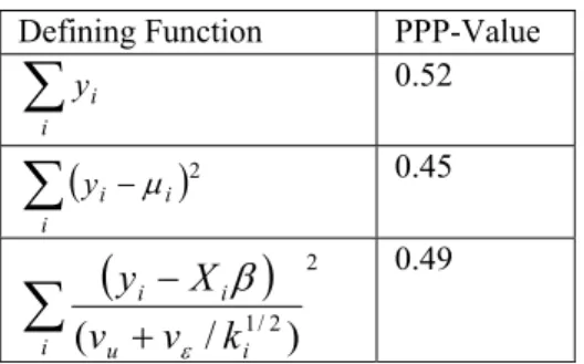
.The first two functions give indications of the fit of the model with respect to the expectation and variance, respectively, by county. We also summarize the resulting PPP-values by taking the mean across the counties to measure the overall fit of the models with respect to expectation and variance. The third is a measure of the overall goodness of fit. You et al (2000) use this measure in their small-area estimation of unemployment.
We use Markov chain Monte Carlo methods to sample from the posterior distribution of θ and the county log insured rate, and to evaluate the model. The implementation is a Metropolis algorithm written in GNU Fortran 77 (Brown and Lovato, 1993). The ‘true’ county log insured rates were integrated out and the parameters were individually updated. Then the county log insured rates,µi, were updated in a
Gibbs step. We chose the Metropolis algorithm to preserve flexibility, since it is not necessary to derive full conditional distributions as it would be for a Gibbs sampler. Thus, changes to the model would require only a modification of the function that computes the likelihood f(y|θ). In this paper we do not take advantage of this feature.
5. Results and Discussion The model we chose is
i i i lpbaskid lpbasadult LINSHR =β0 +β1 +β2 2 i i lhisprt lpbashsp 4 3 β β + + +β5lpoorini(1.0,1.3) . ) 0 . 3 , 0 . 2 ( 7 6lpoorini β lrpopi β + +
That is, the log insured rate in a county is a linear function of: log proportion children, adults ages 35-64, and Hispanics eligible for Medicaid; log proportion Hispanic; log proportion between 100%-130% and 200%-300% of the FPT; and log of the total population. The overall posterior
predictive p-values for the model for counties with sample in ASEC are presented in Table 1. There is no evidence in these overall PPP-values that the model fails with respect to their defining functions. Plots for the PPP-values for the individual counties for the first two functions were plotted versus various variables and examined, similarly to residual plots. Plots of the PPP-values for the means, versus the predictor variables and various demographic variables, failed to show any systematic tendency to over- or under-estimatethe insured rate. The PPP-values for the variance, plotted against sample size, show a lower bound which depends on the sample size. This may indicate that the model for the sampling variance could be improved.
Table 1. PPP-values for the model using the measures in Section 2
The mean, calculated across counties, of the posterior standard deviations of the LINSHR is 0.0085. The mean posterior coefficient of variation (CV) for the uninsured rate is about 5.3 percent.
The posterior means and standard deviation (SD) of
v
u andv
ε are presented in Table 2. The posterior distributions have much smaller variance than the prior distributions; they are clearly dominated by the likelihood. The average ratio of the random-effects variance to the total variance is about 0.6 percent.Table 2. Posterior Means and SD of the Variance Parameters
Variance
Parameter Posterior Mean Posterior SD
u
v
0.000029 0.00041ε
v
0.044 0.0029Recall one possibility in a model like this, without the use of a separate estimate of one of the variance parameters, is that the two components of variance are weakly identified. Examination of the scatterplot of the sample of the joint posterior distribution of the variance parameters,
v
u andv
ε, together with the observation that the priors have relatively large variances, show that the likelihood is well behaved and identification is not a problem. 6. ConclusionWe have formulated a Bayesian model relating the fraction insured to various variables from administrative records and U.S. Census Bureau population estimates. The model has no obvious biases with respect to expectation, though the variance model may still be weak. By estimating the insured rate rather than the uninsured rate we are able to avoid some of the problems we see in the poverty model, specifically the situation where there is no uninsured in sample and the log of that is undefined. The average CV of the estimates, about 5.3 percent, seems sufficiently precise for general use. This depends, of course, on future research regarding the sensitivity of the results to the prior distributions.
Although this type of model would work in a production environment, much needs to be done to make this procedure adequate for the production of reliable estimates. Some of the variables in the data have problems (such as those in the Medicaid data.) While not severe enough to prevent the exploration of their inclusion in a model, these problems should be solved before they are used to make estimates with the U.S. Census Bureau imprimatur. Also, a canon of tests has evolved for small area estimates as produced by the SAIPE project (and inherited by the SAHIE project), which are yet to be done. (See National Research Council (2000).)
More work is also appropriate on the methodology. While the estimation of the log insured rate avoids the problem of censoring counties with no uninsured in sample, there is still an issue, perhaps negligible in the present problem, of the failure of the normality assumption for counties with small sample and proportions of interest close to zero or one. Defining Function PPP-Value
∑
i i y 0.52(
)
∑
− i i i y µ 2 0.45(
)
∑
+
−
i u i i ik
v
v
X
y
2 2 / 1)
/
(
εβ
0.49Fisher and Asher (2000) propose one solution in the context of the estimation of poverty, and Slud (2000) proposes another. We will also consider using external estimates for the variance parameters as in Fay and Herriot (1979), Fisher (1997), or Bell (1999).
There are other sources of data that may be exploited, both as predictors and as responses. The Survey of Income and Program Participation measures insurance coverage as well. Several authors have discussed the differences between these measures and those produced by the ASEC. The fitting and estimation of a multivariate model like this may allow us to make small area estimates for either definition of insurance coverage and to make inferences about the differences between them.
Finally, the form of the model itself may be improved upon. Here the average of three years of ASEC is used as the dependent variable. An alternative is to form a multivariate model with the vector of the three years on the left-hand side of the model, as in You et al (2000) or in Fisher and Campbell (2002). Then we can model the correlation structure of the random effects term and of the sampling error term.
References
Bell, William. 1999. “Accounting for Uncertainty about Variances in Small Area Estimation,” Proceedings of the Section on Survey Research Methods, Alexandria, VA: the American Statistical Association.
Brown, Barry W. and J. Lovato; 1993; RANLIB random number generation library; <http://www.netlib.org/random/ranlib.c.tar.gz>; (accessed: May 2003).
Brown, Richard E., Ying-Ying Meng, Carolyn A. Mendez, and Hongjian Yu. 2001. Uninsured Californians in Assembly and Senate Districts, 2000, UCLA Center for Health Policy Research, Los Angeles, CA.
Centers for Medicare and Medicaid Services; 2002; “FY 1999 MSIS Caveats and Data Limitations;”
<http://cms.hhs.gov/medicaid/msis/caveat99.asp >; (accessed: May 2003).
Fay, Robert E. and Roger A. Herriot. 1979. “Estimates of Income for Small Places: An Application of James-Stein Procedures to Census Data,” Journal of the American Statistical Association, Vol. 74, No. 366, pp. 269-277. Fisher, Robin. 1997. “Methods Used for Small Area Poverty and Income Estimation,” 1997 Proceedings of the Section on Government and Social Statistics, Alexandria, VA: the American Statistical Association.
Fisher, Robin and Jana Asher; 2000; “Alternate CPS Sampling Variance Structures for Constrained and Unconstrained County Models;”
released July 2000; <http://www.census.gov/hhes/www/saipe/techre
p/tech.report.1.revised.pdf>.
Fisher, Robin and Jennifer Campbell. 2002. “Health Insurance Estimates for States,” 2002 Proceedings of the Section on Government and Social Statistics, Alexandria, VA: the American Statistical Association.
Gelfand, Alan E. 1998. “Model Determination Using Sampling-Based Methods,” In Markov Chain Monte Carlo in Practice, (eds W.R. Gilks, et al), pp. 145-161.
Gelman, A. and X. Meng. 1998. “Model Checking and Model Improvement,” In Markov Chain Monte Carlo in Practice, (eds W.R. Gilks, et al), pp. 189-201.
Lazarus, W., B. Foust, and B. Hitt. 2000. The Florida Health Insurance Study Volume 6: The Small Area Analysis, State of Florida, Agency for Health Care Administration, Tallahassee, FL. Lewis, Kimball, M. Ellwood, and J. Czajka. July 1998. “Counting the Uninsured: A Review of the Literature,” The Urban Institute, Assessing the New Federalism: Occasional Paper No. 8, Washington, D.C.
Mills, Robert. 2002. Health Insurance Coverage: 2001. U.S. Census Bureau, Current Population Reports, P60-220. Washington, DC: U.S. Government Printing Office.
National Research Council. 2000. Small Area Estimates of School-Age Children in Poverty: Evaluation of Current Methodology, Panel on Estimates of Poverty for Small Geographic
Areas, Constance F. Citro and Graham Kalton, editors. Committee on National Statistics. Washington, DC: National Academy Press. Popoff, Carole, D.H. Judson, and Betsy Fadali. 2001. “Measuring the Number of People without Health Insurance: A Test of a Synthetic Estimates Approach for Small Areas Using SIPP Microdata,” presented at the 2001 Federal Committee on Statistical Methodology Conference.
Popoff, Carole, B. O’Hara, and D.H. Judson. 2002. “Estimating the Proportion of Uninsured Persons at the County Level: Exploring the Use of Additional Covariates in a Synthetic Estimates System,” 2002 Proceedings of the Section on Government and Social Statistics, Alexandria, VA: the American Statistical Association.
Slud, Eric; 2000; “Models for Simulation & Comparison of SAIPE Analyses;” released 2
May 2000; <http://www.census.gov/hhes/www/saipe/techre
p/saipemod.pdf>.
U.S. Census Bureau; 2003; “Small Area Income and Poverty Estimates Overall Estimation Strategy;”
<http://www.census.gov/hhes/www/saipe/techdo
c/strategy.html>; (accessed: May 2003).
You, Yong, J.N.K. Rao, and Jack Gambino. 2000. “Hierarchical Bayes Estimation of Unemployment Rate for Sub-provincial Regions Using Cross-sectional and Time Series Data,” 2000 Proceedings of the Section on Government and Social Statistics, Alexandria, VA: the American Statistical Association.