A Dissertation by
ICK HOON JIN
Submitted to the Office of Graduate Studies of Texas A&M University
in partial fulfillment of the requirements for the degree of DOCTOR OF PHILOSOPHY
August 2011
A Dissertation by
ICK HOON JIN
Submitted to the Office of Graduate Studies of Texas A&M University
in partial fulfillment of the requirements for the degree of DOCTOR OF PHILOSOPHY
Approved by:
Chair of Committee, Faming Liang Committee Members, David B. Dahl
Samiran Sinha Byung-Jun Yoon Head of Department, Simon Sheather
August 2011 Major Subject: Statistics
ABSTRACT
Statistical Inferences for Models with Intractable Normalizing Constants. (August 2011)
Ick Hoon Jin, B.A., Yonsei University; M.A., Yonsei University Chair of Advisory Committee: Dr. Faming Liang
In this dissertation, we have proposed two new algorithms for statistical infer-ence for models with intractable normalizing constants: the Monte Carlo Metropolis-Hastings algorithm and the Bayesian Stochastic Approximation Monte Carlo algo-rithm. The MCMH algorithm is a Monte Carlo version of the Metropolis-Hastings algorithm. At each iteration, it replaces the unknown normalizing constant ratio by a Monte Carlo estimate. Although the algorithm violates the detailed balance condi-tion, it still converges, as shown in the paper, to the desired target distribution under mild conditions. The BSAMC algorithm works by simulating from a sequence of ap-proximated distributions using the SAMC algorithm. A strong law of large numbers has been established for BSAMC estimators under mild conditions. One significant advantage of our algorithms over the auxiliary variable MCMC methods is that they avoid the requirement for perfect samples, and thus it can be applied to many models for which perfect sampling is not available or very expensive. In addition, although the normalizing constant approximation is also involved in BSAMC, BSAMC can perform very robustly to initial guesses of parameters due to the powerful ability of SAMC in sample space exploration. BSAMC has also provided a general framework for approximated Bayesian inference for the models for which the likelihood function is intractable: sampling from a sequence of approximated distributions with their average converging to the target distribution. With these two illustrated algorithms,
we has demonstrated how the SAMCMC method can be applied to estimate the pa-rameters of ERGMs, which is one of the typical examples of statistical models with intractable normalizing constants. We showed that the resulting estimate is consis-tent, asymptotically normal and asymptotically efficient. Compared to the MCMLE and SSA methods, a significant advantage of SAMCMC is that it overcomes the model degeneracy problem. The strength of SAMCMC comes from its varying truncation mechanism, which enables SAMCMC to avoid the model degeneracy problem through re-initialization. MCMLE and SSA do not possess the re-initialization mechanism, and tend to converge to a solution near the starting point, so they often fail for the models which suffer from the model degeneracy problem.
ACKNOWLEDGMENTS
I am grateful to my dissertation advisor, Prof. Faming Liang and committee members for their interaction and support during my graduate study. This disserta-tion is dedicated to Youn Sil and my family for their endless encouragement, support and love.
TABLE OF CONTENTS
CHAPTER Page
I INTRODUCTION. . . . 1
II EXPONENTIAL RANDOM GRAPH MODELS . . . . 5
A. Introduction . . . 5
B. Parameter Estimation Methods . . . 6
C. Model Degeneracy . . . 8
D. Network Statistics . . . 9
1. Basic Markovian Statistics . . . 10
2. Degree . . . 10
3. Shared Partnership . . . 11
4. Nodal covariates . . . 11
5. Summary . . . 13
III THE MONTE CARLO METROPOLIS-HASTINGS ALGORITHM 14 A. Introduction . . . 14
B. The Monte Carlo Metropolis-Hastings Algorithm . . . 15
1. The Algorithm . . . 15
2. Convergence . . . 19
C. An Example: Exponential Random Graph Models . . . 22
1. High School Student Friendship Network . . . 23
D. MCMH, GIMH and Marginal Inference . . . 26
IV BAYESIAN STOCHASTIC APPROXIMATION MONTE CARLO ALGORITHM . . . . 31
A. Introduction . . . 31
B. Bayesian Stochastic Approximation Monte Carlo Algorithm 32 1. The BSAMC Algorithm . . . 32
2. Convergence . . . 36
C. The Ising Model . . . 44
D. Spatial Models with an Intractable Normalizing Constant . 47 1. Autologistic Model . . . 47
CHAPTER Page V FITTING ERGMS USING VARYING TRUNCATION
STOCHAS-TIC APPROXIMATION MCMC ALGORITHM . . . . 57
A. Introduction . . . 57
B. Stochastic Approximation MCMC with Trajectory Averaging 58 1. Varying Truncation Stochastic Approximation MCMC Algorithm . . . 59
2. Varying Truncation SAMCMC for ERGMs . . . 60
C. Numerical Examples . . . 64
1. Florentine Business Network . . . 66
2. Kapferer’s Tailor Shop Network . . . 69
3. Lazega’s Lawyer Network . . . 74
4. Zachary Karate Network . . . 76
D. A Large Network Example . . . 77
VI CONCLUSION . . . . 83 REFERENCES . . . . 87 APPENDIX A . . . . 97 APPENDIX B . . . . 101 APPENDIX C . . . . 103 VITA . . . . 110
LIST OF TABLES
TABLE Page
I Parameter estimation for the AddHealth school 10 network. . . . . . 24
II RMSEs and AMDs of the MCMLE and MCMH estimates for the ADDHealth School 10 network. . . . . 26
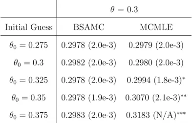
III Parameter estimation for the Ising model with true θ = 0.3. . . . . . 46
IV Parameter estimation for the Ising model with θ0 chosen as the MPLE of θ. . . . . 47
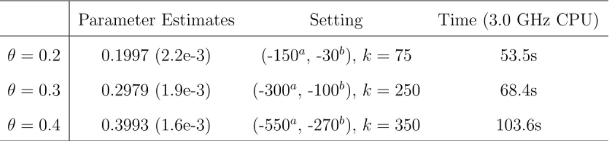
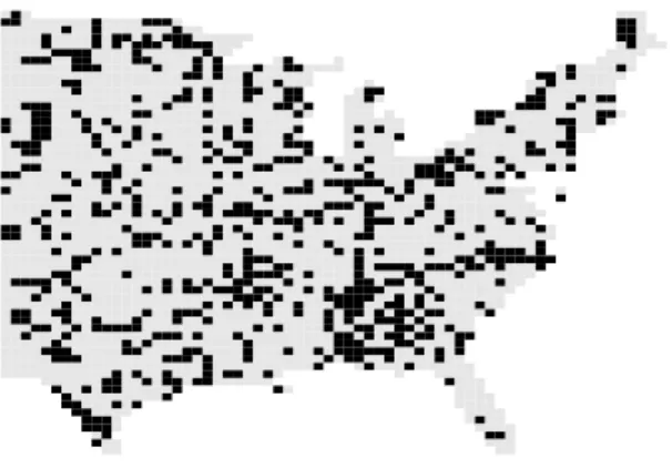
V Parameter estimation for the autologistic model. . . . . 50
VI Estimation of the autonormal model for the wheat yield data. . . . . 56
VII Parameter estimates the Florentine business network. . . . . 67
VIII Estimates ofθ produced by SAMCMC, MCMLE and SSA for the Kapferer’s tailor shop network. . . . . 71
IX Estimates of θ produced by SAMCMC for Kapferer’s tailor Shop network with different starting points. . . . . 72
X Estimates produced by SAMCMC, MCMLE and SSA for Lazega’s lawyer network. . . . . 75
XI Parameter estimates produced by SAMCMC, MCMLE and SSA for the Karate network. . . . . 77
XII Estimates produced by SAMCMC for the high school student friendship network. . . . . 81
LIST OF FIGURES
FIGURE Page
1 Goodness-of-fit(GOF) plots for the high school student friendship
network. . . . . 27 2 US cancer mortality data. . . . . 49 3 Histogram, trace and autocorrelation plots of BSAMC samples
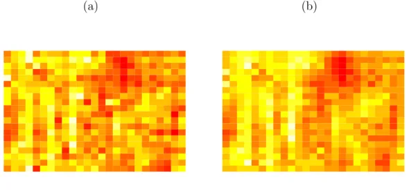
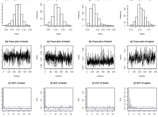
for the autologistic model. . . . . 51 4 Image of the wheat yield data. . . . . 54 5 Histogram, trace and autocorrelation plots of BSAMC samples
for the autonormal model. . . . . 55 6 Social network examples.. . . . 66 7 Goodness-of-fit(GOF) plots for the Florentine business network. . . . 68 8 Trajectories of θ produced by SAMCMC for the Florentine
busi-ness network with different values ofm. . . . . 69 9 Goodness-of-fit(GOF) plots for Kapferer’s tailor shop network. . . . . 71 10 Goodness-of-fit(GOF) plots for Kapferer’s tailor shop network
re-sulted from the runs with the default starting region [−4,4] × [−2,2]2 (row 1), the starting point (−20,0,17) (row 2), and the
starting point (−350,0,350) (row 3). . . . . 73 11 Goodness-of-fit(GOF) plots for Lazega’s lawyer network. . . . . 76 12 Goodness-of-fit(GOF) plots for the Karate network. . . . . 78 13 A large network example: High school student friendship network.. . 79 14 Goodness-of-fit(GOF) plots for the high school student friendship
CHAPTER I
INTRODUCTION
In statistical applications, one often encounters problems of making inference for a model whose likelihood function contains an intractable normalizing constant. Ex-amples of such models include the autologistic model used in ecology study [82], the Potts model used in image analysis [42], the autonormal model used in agriculture ex-periments [9], and the exponential random graph model used in social network study [75], among others.
Suppose we have a dataset X generated from a statistical model with the likeli-hood function
f(x|θ) = 1
κ(θ)exp{−U(x, θ)}, x∈ X, θ∈Θ, (1.1) where θ is the parameter, and κ(θ) is the normalizing constant which depends on θ and is not available in closed form. Let π(θ) denote the prior density imposed on θ. The posterior density of θ is then given by
π(θ|x)∝ 1
κ(θ)exp{−U(x, θ)}π(θ). (1.2)
Since the closed form of κ(θ) is not available, inference for θ poses a great challenge on the current statistical methods.
The MH algorithm cannot be applied to simulate from π(θ|x), because the ac-ceptance probability would involve an unknown ratio κ(θ)/κ(θ0), whereθ0 denotes the
proposed value. To circumvent this difficulty, various approximation methods to the likelihood function or the normalizing constant function have been proposed in the literature. [9] proposed to approximate the likelihood function by a pseudo-likelihood function which is tractable. The method is easy to use, but it typically performs less well for the models for which neighboring dependence is strong. [32] proposed an importance sampling-based approach to approximation κ(θ), which can be briefly described as follows. Let θ∗ denote an initial guess of θ. Let y
1, . . . , ym denote
ran-dom samples simulated fromf(y|θ∗), which can be obtained via a MCMC simulation. Then
logfm(x|θ) = −U(x, θ)−log(κ(θ∗))−log
à 1 m m X i=1 exp{U(yi, θ∗)−U(yi, θ)} ! , (1.3) approaches to logf(x|θ) asm→ ∞. The estimator ˆθ = arg maxθlogfm(x|θ) is called
the MCMLE ofθ. Ifθ(0) lies in the attraction region of true MLE, the method usually produces a good estimate of θ. Otherwise, the method may converge to a suboptimal solution or fail to converge. To alleviate this difficulty, [32] recommended an iterative approach, which drew new samples at the current estimate of θ and then re-estimate: (a) Initialize with a pointθ(0), usually taking to be the maximum pseudo-likelihood
estimator. Set t= 0.
(b) Simulate m auxiliary samples from f(x|θ(t)) using MCMC. (c) Find θ(t+1) = arg max
θlogfm(x|θ).
(d) Stop if a specified number of iterations has been reached, or some other termi-nation criterion has reached. Otherwise, go back to step (b).
Even with this iterative approach, non-convergence is still quite common if θ(0) is far from the true MLE. [46] proposed an alternative Monte Carlo approach to
approxi-mate κ(θ), where κ(θ) is viewed as a marginal density function of the unnormalized distributiong(x, θ) = exp{−U(x, θ)}and estimated using an adaptive kernel smooth-ing approach with Monte Carlo samples.
Toward Bayesian analysis for the model (1.1), a significant step was made by [55], who propose to augment the distribution f(x|θ) by an auxiliary variable such that the normalizing constant ratio κ(θ)/κ(θ0) can be canceled in simulations. Soon, this algorithm was improved by [57], who, based on the idea of parallel tempering [31], proposed the following algorithm—the exchange algorithm:
Exchange Algorithm
• Propose a candidate point θ0 from a proposal distribution denoted byq(θ0|θ, x). • Generate an auxiliary variable y∼f(y|θ0) using a perfect sampler [61].
• Accept θ0 with probability min{1, r(θ, θ0|x)}, where r(θ, θ0|x) = π(θ
0)f(x|θ0)f(y|θ)q(θ|θ0, x) π(θ)f(x|θ)f(y|θ0)q(θ0|θ, x).
Since a swapping operation between (θ, x) and (θ0, y) is involved, the algorithm is called the exchanged algorithm. Both the Møller and the exchange algorithm are called auxiliary variable MCMC algorithms in the literature. The exchange algorithm generally improves the performance of the Møller algorithm, as it avoids an initial estimation step (for θ) that required by the Møller algorithm. See [55] for the role that an initial estimate of θ plays in their algorithm. [57] reported that the exchange algorithm tends to have a higher acceptance probability than the Møller algorithm. Although the Møller and exchange algorithms work well for some discrete models, such as the Ising and autologistic models, they cannot be applied to many other models for which perfect sampling is not available. In addition, even for the Ising and
autologistic models, perfect sampling may be very expensive when the temperature is near or below the critical point.
In Chapter II, we introduce the exponential random graph models (ERGMs) which is one of the well-known statistical models with intractable normalizing con-stants. In Chapter III, we describe the Monte Carlo Metropolis-Hasting algorithm, which replaces the unknown normalizing constant ratio κ(θ)/κ(θ0) by a Monte Carlo estimate to handle intractable normalizing constants problems. In Chapter IV, we il-lustrate the Bayesian Stochastic Approximation Monte Carlo algorithm, which works by simulating from a sequence of approximated distributions using the stochastic approximation Monte Carlo algorithm [50]. for tickling intractable normalizing con-stants problems. In Chapter V, we propose to use the stochastic approximation MCMC (SAMCMC) algorithm to find the maximum likelihood estimator for ERGMs. We conclude our statistical methods for models with intractable normalizing constants in Chapter VI.
CHAPTER II
EXPONENTIAL RANDOM GRAPH MODELS
A. Introduction
The social network is a social structure made of actors (individuals, organizations, etc.) which are interconnected by certain relationship, such as friendship, common interest, financial exchange, etc. The network can be represented in a graph with a node for each actor and an edge for each relation between a pair of actors. This graph representation can provide insight into organizational structures, social behavior pat-terns, and a variety of other social phenomena. Recently, social network analysis has been applied to many other fields, such as biology [71], political science [23], etc. etc. Many statistical models have been proposed in the literature for social network analysis, including the dyadic independence model, the Markov random graph model [27], the exponential random graph model [75], among others. The model of particular interest is the exponential random graph model (ERGM), which allows to include various network dependent structures in the analysis and thus generally improves goodness of fit of social networks. See [68] for an overview of ERGMs.
Consider a social network with n actors. The network can be specified in an n×n-matrix Y= (Yij), where Yij = 1 if there is an edge between nodei and nodej
and 0 otherwise. This matrix is also known as the adjacency matrix. Note that the social network can be either directed or non-directed. The likelihood function of the
ERGM is given by f(y|θ) = 1 κ(θ)exp{ X i∈A θiSi(y)}, (2.1)
where Si(y) denotes a statistic,θi is the corresponding parameter,A specifies the set
of statistics considered in the model, andκ(θ) is the normalizing constant which makes (2.1) a proper probability distribution. An exact calculation of κ(θ) is impossible for all but the smallest networks, as it involves a sum over all possible networks. In the rest of this paper, we will let S(y) = (S1(y), . . . , Sd(y)) denote the vector of
d statistics considered in the model, and let θ = (θ1, . . . , θd) denote the vector of d
parameters of the model.
Parameter estimation for ERGMs suffers from two difficulties. The first difficulty is due to the intractability of κ(θ), and the second is the so-called model degeneracy problem. They will be discussed in sequel as follows.
B. Parameter Estimation Methods
Because κ(θ) in (2.1) is intractable, estimation of θ has put a great challenge on the current statistical methods. Several methods have been proposed in the literature, including the maximum pseudo-likelihood estimation (MPLE) method [76], Monte Carlo maximum likelihood estimation (MCMLE) method ([32], [40]), stochastic ap-proximation (SA) method [74], among others.
The MPLE method analyzes ERGMs with a simplified, analytic form of the likelihood function under the assumption of dyadic independence. The properties of this method has been studied by many authors, see e.g., [22], [25], [51] and [80]. MPLE is intrinsically highly dependent on the observed network. It usually works well for the networks with low dependence structure, but may produce substantially biased estimates for the networks with high dependency.
The MCMLE method originates in [32], whose basic idea is to approximate the normalizing constant κ(θ) using Monte Carlo samples. It is known that the perfor-mance of this method depends on the choice of an initial guess. If the initial guess is near the MLE, it can produce a good estimate of θ. Otherwise, it may converge to a local optimal solution or even fail to converge. To alleviate this difficulty, [32] recommended an iterative approach, which drew new samples at the current estimate of θ and then re-estimate. Even with this iterative procedure, as pointed out by [7], non-convergence is still quite common for ERGMs.
With some simple manipulations, it is easy to show that maximizing the likeli-hood function (2.1) is equivalent to solve the system of equations
Eθ(S(Y)) =S(yobs), (2.2)
where the expectation is taken with respect to the distribution f(y|θ) as specified in (2.1). The rationale underlying this reformulation is the exponential family theory ([6]; [14]), which says that the MLE of (2.1), if existing, is the unique vector ˆθ such that (2.2) holds. [74] applies the stochastic approximation algorithm [64] to solve (2.2) for θ. In this paper, we call this method the SSA method. One iteration of SSA consists of two main steps:
(a) (Independence network generation) Generate an independent sample y(k+1) from the distributionf(y|θ(k)): Starting with a random graph in which each arc variable Yij is determined independently with a probability 0.5 for the values
0 and 1; and then updating the random graph using the Gibbs sampler [30] or the MH algorithm [36] and [54].
(b) (Estimate updating) Set
θ(k+1) =θ(k)−a
kD−1
¡
where {ak} denotes a positive sequence converging to 0, D denotes a
pre-estimated covariance matrix ofS(Y) at the initial estimateθ(1), ¯y
k+1 = 1−yk+1 denotes the complementary network of yk+1 (with each cell of the adjacency matrix of yk+1 being switched from 0 to 1 and vice versa),
U(yk+1,y¯k+1) = P(¯yk+1|yk+1)S(¯yk+1) + (1−P(¯yk+1|yk+1))S(yk+1), andP(¯yk+1|yk+1) denotes the MH acceptance probability of the transition from
yk+1 to ¯yk+1.
A major shortcoming of SSA is its inefficiency in generating independent network samples. The number of updating steps for generating each sample yk+1 is in the order of 100n2, where n denotes the total number of nodes included in the network. This is very time consuming when n is large.
C. Model Degeneracy
The model degeneracy problem [34] refers to the phenomenon that for some con-figurations of θ, the model (2.1) produces networks that are either full (every tie exists) or empty (no ties exist) with probability close to one. For example, the mod-els with basic Markovian statistics (e.g., the number of triangles) often suffer from the model degeneracy problem. When one edge is added to or removed from the network, the values of the basic Markovian statistics can change a lot while the val-ues of other statistics do not change proportionally, so the dyadic dependence effects amplify quickly and the model tend to be degenerated. When the observed network is fitted by such a model, the MCMLE and SSA method may produce a degenerated estimate of θ (i.e., the estimate falls in a degeneracy region) if the starting value is in or close to a degeneracy region. In this case, the resulting model will not provide
a good fitting to the network. The reason why MCMLE and SSA often fail for the model degeneracy problem is due to their local convergence property, i.e., they tend to converge to a local optimal solution near the starting point.
As pointed out by [35], the model degeneracy problem can also be viewed as a model mis-specification problem. A solution to avoid this problem is to specify a model whose parameter space contains no or less degeneracy regions. However, this is often more difficult than usual. For a linear model, the mis-specification can be diagnosed by comparing observed to predicted values; but for ERGMs, if the model is mis-specified, the analyst can be left with little information to help guide the re-specification of the model.
D. Network Statistics
Recall the likelihood function given in (2.1). To define ERGMs, it is necessary to specify the sufficient statistics S(y) explicitly. Since a large number of specifications are available for ERGMs, we consider only several commonly used statistics in this article, including basic Markovian statistics [27], the degree distribution, the edge-wise shared partnership distribution [75], and nodal covariates. The basic Markovian statistics, which consist of edge counts, k2-star, k3-star, and triangle counts, describe the basic structure of social networks. The degree distribution and the edgewise shared partnership distribution describe the higher order transitivity of social net-works. Nodal covariates introduce actor attributes into ERGMs. See [68] and [69] for overviews of ERGMs.
1. Basic Markovian Statistics
The edge counts, denoted by S1(y), is the count of edges contained in the social network y. If one node connects to other two nodes, it is called 2-star. In the same manner, if one node connects to other three nodes, it is called 3-star. The counts of 2-stars and 3-star are called k2-star and k3-star, and denoted by S2(y) and S3(y), respectively. If node ’a’ connects to node ’b’, node ’b’ connects to node ’c’, and node ’c’ connects to node ’a’ simultaneously, then the nodes ’a’, ’b’ and ’c’ form a triangle. The count of triangles is denoted by T(y). Mathematically, the statistics Sk(y) (k= 2,3) andT(y) can be calculated by
S1(y) = X 1≤i<j≤G yij; Sk(y) = X 1≤i≤G µ yi+ k ¶ , k= 2,3; T(y) = X 1≤i<j<h≤G yijyihyjh, (2.4) where yi+ denotes the degree of nodei.
2. Degree
Let Di(y) denote the number of nodes whose degree, the number of edges
inci-dent to the node, equals i. The statistics D0(y), . . . , DG−1(y) satisfy the constraint
PG−1
i=0 Di(y) = G, and the edge count statistic can be re-expressed as S1(y) = 1
2
PG−1
i=1 iDi(y).
The geometrically weighted degree statistic ([38], [40], and [75]) is defined by u(y|τ) =eτ G−2 X i=1 ½ 1− ³ 1−e−τ ´i¾ Di(y), (2.5)
where the additional parameter τ specifies the decreasing rate of weights put on the higher order terms. Following [39], we fix τ to be a constant throughout this paper. Although treating τ as an unknown parameter can potentially improve the model fitting, the distribution (2.1) will no longer satisfy the form of exponential family.
Rather it belongs to a curved exponential family.
3. Shared Partnership
Let EPk(y) denote the number of unordered pairs (i, j) for which i and j have
ex-actlyk common neighbors andYij = 1. LetDPk(y) denote the number of unordered
pairs (i, j) for which i and j have exactly k common neighbors regardless the value of Yij. In the literature, EPk(y) is called the edge-wise shared partnership
statis-tic and DPk(y) the dyad-wise shared partnership statistic. They satisfy the
con-straint PGk=0−2EPk(y) = S1(y) and PG−2 k=0 DPk(y) = ¡n 2 ¢
. The geometrically weighted edgewise shared partnership (GWESP) statistic and geometrically weighted dyadwise shared partnership (GWDSP) statistic ([38], [40], and [75]) are defined by
v(y|τ) = eτ G−2 X i=1 ½ 1− ³ 1−e−τ ´i¾ EPi(y), (2.6) w(y|τ) = eτ G−2 X i=1 ½ 1− ³ 1−e−τ ´i¾ DPi(y), (2.7)
where the parameterτ specifies the decreasing rate of weights put on the higher order terms. As for the GWD statistic, τ is fixed to a constant throughout this paper.
4. Nodal covariates
Nodal covariates represent specific features of a node. Let Xi denote a covariate of
node i. All nodal covariates can be expressed as a dyadic independence statistic of the form
X X
i<j
yijh(Xi, Xj) (2.8)
for a suitably chosen function h(Xi, Xj) [39]. In this paper, we consider a few types
factor effect and absolute difference factor effect. The latter three are usually used for categorical factors and their statistics take values of 0 or natural numbers.
The main factor effect directly adds covariates of nodes iand j; that is,
h(Xi, Xj) = Xi +Xj. (2.9)
For each edge, the nodal factor effect gives the node a score according to the counts of endpoints which have the specified factor level. It is defined by
h(Xi, Xj) =
2, if bothi and j have the specified factor level, 1, if exactly one ofi, j has the specified factor level, 0, if neitheri nor j has the specified factor level.
(2.10)
Since the sum of nodal factor effects for all levels are equal to twice the edge counts of the network, one level must be excluded in nodal factor effects to remove the linear dependency.
The homophily factor effect gives each edge a score of 0 or 1, depending on whether or not the two endpoints have the same factor level. There are two types of homophily factor effects: uniform homophily factor effect and differential homophily factor effect. The former is defined by
h(Xi, Xj) =
1, if i and j have the same factor level, 0, otherwise,
(2.11)
and the latter is defined by
h(Xi, Xj) =
1, if i and j have the specified factor level, 0, otherwise.
(2.12)
dif-ferences in covariates tend to connect by edges. To incorporate this effect into the models, we add a new statistic, the so-called absolute difference factor effect, into the model. This effect is defined by
h(Xi, Xj) =
1 if |Xi−Xj|=C for some nonzero constant C,
0 otherwise.
(2.13)
If C = 0, it would introduce a linear dependence with the homophily factor effect.
5. Summary
In summary, the network statistics can be generally classified into two groups: dyadic dependent and dyadic independent [35], where a dyad refers to a pair of nodes. Dyadic independence means there are no direct dependence among dyads; that is, the state of a dyad is independent of the state of other dyads. The edge counts and nodal covariate terms are dyadic independent statistics. Dyadic dependence means the state of one dyad stochastically depends on the state of other dyad. An example is “the friend of my friend is also my friend”— edges in dyad (i, j) and (j, k) increase the probability of relation in dyad (i, k). Thek-star, triangle, degree and share partnership statistics are dyadic dependent statistics. The dyadic dependent statistics tend to cause the model degeneracy problem.
CHAPTER III
THE MONTE CARLO METROPOLIS-HASTINGS ALGORITHM
A. Introduction
In this chapter, we propose a new algorithm, the so-called Monte Carlo Metropolis-Hastings (MCMH) algorithm, for sampling from distributions with intractable nor-malizing constants. The MCMH algorithm is a Monte Carlo version of the Metropolis-Hastings algorithm. At each iteration, it replaces the unknown normalizing constant ratio κ(θ)/κ(θ0) by a Monte Carlo estimate. Under mild conditions, we show that the MCMH algorithm can still converge to the desired stationary distribution π(θ|x). Unlike the Møller and exchange algorithms, the MCMH algorithm avoids the require-ment for perfect sampling, and thus can be applied to many statistical models for which perfect sampling is not available or very expensive.
The remainder of this chapter is organized as follows. In Section B, we describe the MCMH algorithm. In Section C, we test the MCMH algorithm on social network models. In Section D, we discuss the relation between MCMH and the group inde-pendence MH algorithm introduced by [8], and the potential applications of MCMH in marginal inference.
B. The Monte Carlo Metropolis-Hastings Algorithm 1. The Algorithm
Consider the problem of sampling from the distribution (1.2). Let θt denote the
current draw of θ by the algorithm. Let y1(t), . . . , y(mt) denote the auxiliary samples
simulated from the distribution f(y|θt), which can be drawn by either a MCMC
algorithm or an automated rejection sampling algorithm [13]. The MCMH algorithm works by iterating between the following steps:
Monte Carlo MH Algorithm I
1. Drawϑ from some proposal distribution Q(θt, ϑ).
2. Estimate the normalizing constant ratioR(θt, ϑ) =κ(ϑ)/κ(θt) by
b Rm(θt,yt, ϑ) = 1 m m X i=1 g(y(it), ϑ) g(yi(t), θt) ,
where g(y, θ) = exp{−U(y, θ)}, and yt = (y(1t), . . . , y(mt)) denotes the collection
of the auxiliary samples.
3. Calculate the Monte Carlo MH ratio ˜ rm(θt,yt, ϑ) = 1 b Rm(θt,yt, ϑ) g(x, ϑ)π(ϑ) g(x, θt)π(θt) Q(ϑ, θt) Q(θt, ϑ) , where π(θ) denotes the prior distribution imposed on θ.
4. Setθt+1 =ϑ with probability ˜α(θt,yt, ϑ) = min{1,r˜m(θt,yt, ϑ)}, and setθt+1 = θt with the remaining probability.
5. If the proposal is rejected in step 4, set yt+1 = yt. Otherwise, draw samples
yt+1 = (y1(t+1), . . .,ym(t+1)) from f(y|θt+1) using either a MCMC algorithm or an
Since the algorithm involves a Monte Carlo step to estimate the unknown nor-malizing constant ratio, it is termed as “Monte Carlo MH”. Clearly, the samples {(θt,yt)} forms a Markov chain whose transition kernel is given by
˜ Pm(θ,y;dϑ, dz) = ˜α(θ,y, ϑ)Q(θ, dϑ)fϑm(dz) +δθ,y(dϑ, dz) £ 1− Z Θ×Y ˜ α(θ,y, ϑ0)Q(θ, dϑ0)fm ϑ0(dz0) ¤ = ˜α(θ,y, ϑ)Q(θ, dϑ)fϑm(dz) +δθ,y(dϑ, dz) £ 1− Z Θ ˜ α(θ,y, ϑ0)Q(θ, dϑ0)¤, (3.1) where fm
θ (y) =f(y1, . . . , ym|θ) denotes the joint density of y1, . . . , ym.
In general, if {(Xt, Yt)} forms a Markov chain, then the marginal path {Xt}
forms an adaptive Markov chain for which each state depends all of its past states; that is, Xt depends on Xt−1, . . . , X1, X0 for all t ≥ 1. For the MCMH-I algorithm,
the transition kernel of the marginal chain {θt} is given by
˜ Pm(θt, dϑ) = Z Y Z Y ˜ Pm(θt,yt;dϑ, dz)fθmt(dyt) = Z Y ˜ α(θt,yt, ϑ)Q(θt, dϑ)fθmt(dyt) +δθt(dϑ) £ 1− Z Θ×Y ˜ α(θt,yt, ϑ0)Q(θt, dϑ0)fθmt(dyt) ¤ . (3.2)
It is easy to see that ˜Pm(θt, dϑ) is independent of {θt−1, . . . , θ0}. This implies that the ergodicity of {θt} can be analyzed as a non-adaptive Markov chain. However, in
Theorem B.2 we still show that {θt} has the same stationary distribution as the time
homogeneous Markov chain under the framework of adaptive Markov chain (see e.g., [66]). Note that the independence of ˜Pm(θt, dϑ) on past states is not generally true
for all marginal Markov chains. It is true for MCMH-I as for which yt is generated from fθt(y), which implies that yt is independent of θ0, . . . , θt−1 conditional on θt.
equilib-rium, if a MCMC algorithm is used for generating the auxiliary samples. To ensure this requirement to be satisfied, we propose to choose the initial auxiliary sample at each iteration through an importance resampling procedure; that is, set y(0t+1) =y(it) with a probability proportional to the importance weight
wi =g(yi(t), θt+1)/g(y(it), θt). (3.3)
As long as y0(t+1) follows correctly from the conditional distribution f(y|θt+1), this procedure ensures that all samples, yt+1, yt+2, yt+3, . . ., drawn in the followed it-erations will follow correctly from the respective conditional distributions, provided that θ does not change drastically at each iteration. Note that the resampling proce-dure may introduce a (probably very slight) dependence on the previous samples. In practice, we may ignore this dependence, especially when m is large.
Regarding the choice ofm, we note that m may not necessarily be very large in practice. In our experience, a value between 20 and 50 may be good for most problems. It seems that the random errors introduced by the Monte Carlo estimate ofκ(θt)/κ(ϑ)
can be smoothed out by path averaging over iterations. This is particularly true for parameter estimation.
The MCMH algorithm can have many variants. A simple one is to draw auxiliary samples at each iteration, regardless of acceptance or rejection of the last proposal. This variant be described as follows:
Monte Carlo MH Algorithm II
1. Drawϑ from some proposal distribution Q(θt, ϑ).
2. Draw auxiliary samples yt = (y1(t), . . . , ym(t)) from f(y|θt) using a MCMC
3. Estimate the normalizing constant ratioR(θt, ϑ) =κ(ϑ)/κ(θt) by b Rm(θt,yt, ϑ) = 1 m m X i=1 g(y(it), ϑ) g(yi(t), θt) .
4. Calculate the Monte Carlo MH ratio ˜ rm(θt,yt, ϑ) = 1 b Rm(θt,yt, ϑ) g(x, ϑ)π(ϑ) g(x, θt)π(θt) Q(ϑ, θt) Q(θt, ϑ) .
5. Set θt+1 =ϑ with probability ˜α(θt,yt, ϑ) = min{1,r˜m(θt,yt, ϑ)}and set θt+1 = θt with the remaining probability.
MCMH-II has a different Markovian structure from MCMH-I. In MCMH-II,{θt}
forms a Markov chain with the transition kernel given by ˜ Pm(θ, dϑ) = Z Y ˜ α(θ,y, ϑ)Q(θ, dϑ)fθm(dy) +δθ(dϑ) £ 1− Z Θ×Y ˜ α(θ,y, ϑ0)Q(θ, dϑ0)fm θ (dy) ¤ , (3.4)
which is identical to the marginal transition kernel (3.2) except for notations. Hence, the two algorithms will have the same convergence rate for {θt}.
Intuitively, one may expect that MCMH-I converges slowly than MCMH-II, as the former recycles the auxiliary samples when rejection occurs and thus the successive samples generated by it may have significantly higher correlation than those generated by the latter. In fact, the random error of Rbm(θt,yt, ϑ) depends mainly on θt and ϑ
instead of yt when m is large. This may help us to understand why MCMH-I and MCMH-II show the same convergence rate in numerical examples.
Similar to MCMH-II, we can propose another variant of MCMH, which, in step 2, draws auxiliary samples from f(y|ϑ) instead of f(y|θt). Then
b R∗ m(θt,yt, ϑ) = 1 m m X i=1 g(yi(t), θt) g(y(it), ϑ),
forms an unbiased estimator of the ratio κ(θt)/κ(ϑ), and the Monte Carlo MH ratio can be calculated as ˜ rm∗ (θt,yt, ϑ) =Rbm∗(θt,yt, ϑ) g(x, ϑ)π(ϑ) g(x, θt)π(θt) Q(ϑ, θt) Q(θt, ϑ) .
In addition tof(y|θt) orf(y|ϑ), the auxiliary samples can also be generated from
a third distribution which has the same support set as f(y|θt) and f(y|ϑ). In this
case, the ratio importance sampling method ([18], [78]) can be used for estimating the normalizing constant ratio κ(θt)/κ(ϑ). The existing normalizing constant ratio
estimation techniques, such as bridge sampling [53] and path sampling [28], are also applicable to MCMH with an appropriate strategy for generating auxiliary samples.
2. Convergence
In this subsection, we first prove the ergodicity of MCMH-II; that is, showing kP˜k
m(θ0,·)−π(·|x)k →0, asm→ ∞ and k → ∞,
where k denotes the number of iterations, π(·|x) denotes the target distribution de-fined in (1.2), and k · k denotes the total variation norm as specified in [77]. Then, based on the theory of adaptive Markov chain [4], we show that MCMH-I has the same stationary distribution as MCMH-II. The main results are presented below, whose proofs can be found in Appendix A. Extension of these results to other vari-ants of MCMH is straightforward. Define γm(θ,y, ϑ) = R(θ, ϑ) b R(θ,y, ϑ).
λm =|log(γm(θ,y, ϑ))|, and define ρ(θ) = 1− Z Θ×Y ˜ αm(θ,y, ϑ)Q(θ, dϑ)fθm(dy),
which represents the mean rejection probability of a MCMH-II transition from θ. To show the convergence of MCMH-II, we also consider the transition kernel
P(θ, ϑ) = α(θ, ϑ)Q(θ, ϑ) +δθ(dϑ) £ 1− Z Θ α(θ, ϑ)Q(θ, ϑ)dϑ¤,
which is induced by the proposal Q(·,·). In addition, we assume the following condi-tions:
(A1) Assume that P defines an irreducible and aperiodic Markov chain such that πP =π, and for any θ0 ∈Θ, limk→∞kPk(θ0,·)−π(·|x)k= 0.
(A2) For any (θ, ϑ)∈Θ×Θ,
γm(θ,y, ϑ)>0, fθm(·)−a.s.
(A3) For any θ ∈Θ and any² >0, lim m→∞Q(θ, f m θ (λm(θ,y, ϑ)> ²)) = 0, where Q(θ, fm θ (λm(θ,y, ϑ)> ²)) = R {(ϑ,y):λm(θ,y,ϑ)>²}f m θ (dy)Q(θ, dϑ).
The condition (A1) can be simply satisfied by choosing an appropriate proposal dis-tribution Q(·,·), following from the standard theory of the Metropolis-Hastings algo-rithm [77]. The condition (A2) assumes that the distributionsf(y|θ) andf(y|ϑ) have a reasonable overlap such that Rb forms a reasonable estimator of R. The condition (A3) is equivalent to assuming that for any θ ∈ Θ and any ² > 0, there exists a
positive integer M such that for any m > M,
Q(θ, fθm(λm(θ,y, ϑ)> ²))≤².
It essentially requires that R(θ,b y, ϑ) is a consistent estimator of R(θ,y, ϑ) and the stepsize of the proposalQ(θ, ϑ) is reasonably small, i.e.,ϑlies in a small neighborhood of θ.
Lemma B.1 states that the marginal kernel ˜Pm has a stationary distribution. It
is proved in a similar way to Theorem 1 of [3]. The relation between this work and [8] and [3] will be discussed in Section 5.
Lemma B.1 Assume (A1) and (A2) hold. Then for any m ∈ N such that for any
θ ∈ Θ, ρ(θ) > 0, P˜m is also irreducible and aperiodic, and hence there exists a
stationary distribution π˜m(θ|x) such that for any θ0 ∈Θ, lim
k→∞k ˜
Pmk(θ0,·)−π˜m(·|x)k= 0.
Lemma B.2 concerns the distance between the kernel ˜Pm and the kernel P. It
states that the two kernels can be arbitrarily close to each other, provided that m is large enough.
Lemma B.2 Assume (A3) holds. Let ² ∈ (0,1]. Then for any θ ∈ Θ, there exists
M(θ)∈N such that for any ψ : Θ →[−1,1] and any m > M(θ), |P˜mψ(θ)−P ψ(θ)| ≤4².
Theorem B.1 concerns the ergodicity of MCMH-II. It states that the kernel ˜Pm
asymptotically shares the same stationary distribution with the MH kernel P.
Theorem B.1 Assume the conditions (A1), (A2)and(A3)hold for MCMH-II. Then
that for any m > M(ε, θ0) and k > K(ε, θ0, m)
kP˜mk(θ0,·)−π(·|x)k ≤ε, where π(·|x) denotes the posterior density of θ.
Theorem B.2 Assume the conditions (A1), (A2) and (A3) hold for MCMH-I. Then
the marginal chain {θt} induced by MCMH-I has the same stationary distribution as
the Markov chain {θt} induced by MCMH-II.
Theorem B.1 and Theorem B.2 imply, by standard MCMC theory (see, e.g., [77]), that for an integrable function h(θ), the path averaging estimator Pnk=1h(θk)/n will
converge to its posterior mean almost surely; that is, as k→ ∞, 1 n n X k=1 h(θk)→ Z h(θ)π(θ|x)dθ, a.s.,
provided that R |h(θ)|π(θ|x)dθ < ∞ and m has been sufficiently large so that the error in replacing ˜πm(θ|x) by π(θ|x) is ignorable. Here ˜πm denotes the stationary
distribution established in Lemma B.1 for a fixed value of m.
C. An Example: Exponential Random Graph Models
Based on the statistics defined , we consider three ERGMs with respective likelihood functions given by
f(x|θ) = 1
κ(θ)exp{θ1e(x) +θ2u(x|τ)}, (Model 1), f(x|θ) = 1
κ(θ)exp{θ1e(x) +θ2v(x|τ)}, (Model 2), f(x|θ) = 1
κ(θ)exp{θ1e(x) +θ2u(x|τ) +θ3v(x|τ)}, (Model 3).
was imposed on θ, whered is the dimension of θ, and Id is an identity matrix of size
d×d. Then, MCMH can be applied to simulate from the posterior. The proposal distribution Q(·,·) used here is a Gaussian random walk proposal Nd(θt, s2Id), and
s is called the step size. In all simulations of this section, s was fixed to 0.2. Each auxiliary sample is generated through a cycle of Metropolis-within-Gibbs updates.
1. High School Student Friendship Network
The data was collected during the first wave (1994-1995) of National Longitudinal Study of Adolescent Health(AddHealth) through a stratified sampling survey in the U.S. schools containing grades 7 through 12. To collect the data, the school admin-istrator made a roster of all students and asked students to nominate five close male and female friends. Students were allowed to nominate their friends who were not in their school. The students may choose not to nominate if they did not have enough number of close male or female friends. The detailed description of the data can be found in [62], [79], or at http://www.cpc.unc.edu/projects/addhealth. The full dataset contains 86 schools and 90,118 students. In this paper, only the subnetwork for school 10, which has 205 students, is analyzed. Also, only the undirected network for the case of mutual friendship are considered.
MCMH-I was applied to this network with m = 20. For each model, MCMH-I was run 5 times independently. Each run started with a random point and consisted of 5,000 iterations, where the first 1000 iterations were discarded for the burn-in process and the samples collected from the remaining iterations were used for estimation. The results were summarized in Table I.
For comparison, the MCMLE was also applied to this example. The software we used for MCMLE is an R package ergm by [41]. MCMLE was also run 5 times for each model of this example. Each run consisted of 25 iterations with 6,500
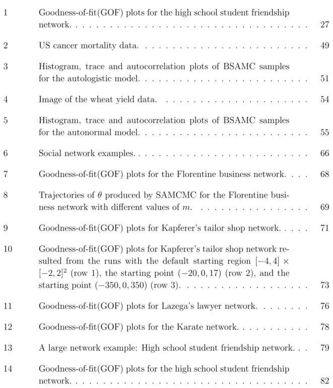
aux-iliary networks being generated at each iteration. In the ergm package, the auxiliary networks was simulated using the tie-no-tie sampler with both the number of burnin and the number of interval steps being set to 20,000. Under this setting, a total of 1.3×10⁸(= 20,000×6,500) MH updates (each for one edge) are needed for generating 6500 networks at each iteration of MCMLE. The results are summarized in Table I. It indicates that MCMLE costs longer CPU times than MCMH-I for this example. All computations for this example were done on a 3.0GHz Intel Core 2 Duo computer. Table I. Parameter estimation for the AddHealth school 10 network. The estimates were calculated by averaging over 5 independent runs with the standard de-viations reported in the parentheses. CPU: the CPU time (in minutes) cost by a single run on a 3.0GHz Intel Core 2 Duo computer.
Method Terms Model 1 Model 2 Model 3
MCMH Edge Counts -3.922(7.0e-3) -5.607(1.3e-2) -5.507(3.7e-2)
GWD -1.545(1.6e-2) -0.101(3.7e-2)
GWESP 1.889(1.2e-2) 1.821(2.4e-2)
CPU(m) 33.6 33.5 60.1
MCMLE Edge Counts -3.977(5.3e-2) -5.388(9.3e-3) -5.170(1.5e-2)
GWD -1.297(4.3e-2) -0.227(6.1e-3)
GWESP 1.711(7.8e-3) 1.589(1.5e-2)
CPU(m) 45.1 48.9 70.8
To assess accuracy of the MCMH estimates, the following procedure was proposed in a similar spirit to the parametric bootstrap method [26], which calculated the root mean squared errors (RMSEs) of the estimates ofSa(x)’s. Since the statistics{Sa(x) :
a ∈A} are sufficient forθ, if an estimate θbis accurate, thenSa(x)’s can be reversely
estimated by simulated networks from the distributionf(x|θ). The procedure consistsb of three steps:
(a) Given the estimate ˆθ, simulateK networks,x1, . . . , xK, independently using the
Gibbs sampler.
(b) Calculate the statistics Sa(x), a∈A for each of the simulated networks.
(c) Calculate RMSE by following equation.
RMSE(Sa) = v u u tXK i=1 £ Sa(xi)−Sa(x) ¤2 /K, a ∈A, (3.5)
where Sa(x) is the corresponding statistic calculated from the network x.
In addition to RMSE, we also calculate the absolute mean difference (AMD) for each statistic, AMD(Sa) = ¯ ¯ ¯ ¯ ¯ 1 K K X i=1 Sa(xi)−Sa(x) ¯ ¯ ¯ ¯ ¯.
With simple manipulations, it is easy to show the following equalities hold at the MLE of θ:
Eθ[Sa(X)] =Sa(x), ∀ a∈A, (3.6)
where Eθ[·] denotes the expectation with respect to the distribution f(x|θ) given in
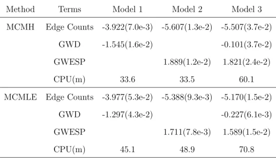
(2.1). Hence, AMD also provides a measure for the quality of the estimate of θ. For each of the estimates shown in Table I, the RMSEs and AMDs were calculated with K = 1000 and summarized in Table II. The results indicate that MCMH-I produced much more accurate estimates than MCMLE for all the three models. We note that [39] have also applied MCMLE to model 1 and model 2 for this network. Their estimate for model 2 is similar to ours, but their estimate for model 1 is much worse than ours. [39] reported the estimate of model 1 as (−1.423,−1.305), for which the RMSE values are 4577.2 for the edge count and 90.011 for GWD. MCMH-I was also run with m= 50 for this network. The results were very similar.
Table II. RMSEs and AMDs of the MCMLE and MCMH estimates for the ADDHealth School 10 network.
Model 1 Model 2 Model 3
Method Terms RMSE AMD RMSE AMD RMSE AMD
MCMH Edge Counts 32.449 2.672 26.998 2.252 22.993 10.821
GWD 16.222 0.357 12.519 3.518
GWESP 28.269 0.945 30.531 11.333
MCMLE Edge Counts 50.046 42.151 41.305 29.599 87.158 76.948
GWD 26.964 24.497 27.609 25.277
GWESP 33.180 14.568 70.470 56.189
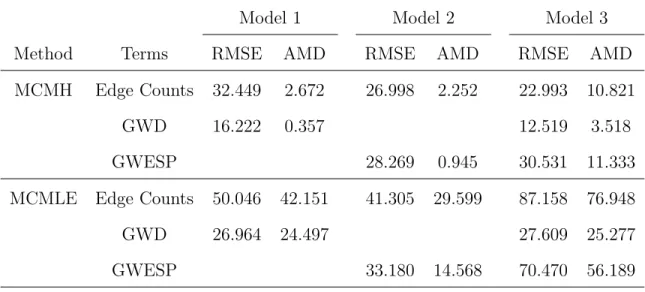
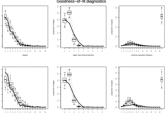
Finally, we assessed accuracy of the model estimates using the goodness-of-fit (GOF) plots [39]. The GOF plot shows the distribution (through box-plots and confidence intervals) of three sets of statistics, the degree distribution, the edgewise shared partnership distribution and the geodesic distance distribution, for the fitted model. If the statistics of the observed network, which are represented by a solid line in the GOF plots, falls into the confidence intervals of the fitted model, then the fitting is considered good. The closer the solid line is to the center of the box-plots, the better the fitting is. Figure 1 compares the GOF plots for the two estimates of model 3. It indicates that MCMH-I provides a better fitting for the network than MCMLE. For other two models, GOF plots (omitted here) also indicate that MCMH-I works better than MCMLE for this example.
D. MCMH, GIMH and Marginal Inference
In the literature, there is one algorithm, namely, grouped independence MH (GIMH) [8], which is similar in spirit to the MCMH algorithm. GIMH is designed for marginal
0 12 3 45 67 8 910 12 14 16 0.0 0.1 0.2 0.3 degree propor tion of nodes 0 1 2 3 4 5 6 7 8 0.0 0.1 0.2 0.3 0.4 0.5 0.6
edge−wise shared partners
propor tion of edges 123456789 11 13 15 17 19 0.0 0.2 0.4 0.6 0.8
minimum geodesic distance
propor tion of dy ads Goodness−of−fit diagnostics 0 12 3 45 67 8 910 12 14 16 0.00 0.05 0.10 0.15 0.20 0.25 0.30 degree propor tion of nodes 0 1 2 3 4 5 6 7 8 0.0 0.1 0.2 0.3 0.4 0.5 0.6
edge−wise shared partners
propor tion of edges 123456789 11 13 15 17 19 0.0 0.1 0.2 0.3 0.4 0.5 0.6 0.7
minimum geodesic distance
propor
tion of dy
ads
Goodness−of−fit diagnostics
Fig. 1. Goodness-of-fit(GOF) plots for the high school student friendship network. Row 1: MCMH-I estimate; Row 2: MCMLE. The solid line shows the observed network statistics, and the box-plots represent the distributions of simulated network statistics.
inference from a joint distribution.
Let π(θ, y) denote a joint distribution. Suppose that one is interested in the marginal distribution π(θ). For example, in Bayesian statistics, θ could represent a parameter of interest and y a set of missing data or latent variables. As implied by the Rao-Blackwell theorem [11], a basic principle in Monte Carlo computation is to carry out analytical computation as much as possible. Motivated by this principle, [8] proposed to replace π(θ) by its Monte Carlo estimate in simulations when the analyt-ical form of π(θ) is not available. Let y= (y1, . . . , ym) denote a set of independently
identically distributed (iid) samples drawn from a trial distribution qθ(y). It follows
from the standard theory of importance sampling that
e π(θ) = 1 m m X i=1 π(θ, yi) qθ(yi) , (3.7)
forms an unbiased estimate of π(θ). In simulations, GIMH treats π(θ) as a knowne
target density, then simulate from it using the Metropolis-Hastings algorithm. Let θt
denote the current draw of θ, and let yt= (y1(t), . . . , ym(t)) denote a set of iid auxiliary
samples drawn from qθ(y). One iteration of GIMH consists of the following steps:
Group Independence MH Algorithm
• Generate a new candidate point θ0 from a proposal distribution T(θ0|θ
t).
• Draw m iid samples y0 = (y0
1, . . . , ym0 ) from the trial distribution qθ0(y). • Accept the proposal with probability
min ½ 1,eπ(θ 0) e π(θt) T(θt|θ0) T(θ0|θ t) ¾ .
If it is accepted, set θt+1 = θ0 and yt+1 = y0. Otherwise, set θt+1 = θt and
The convergence of the GIMH algorithm has been studied by [3] under similar conditions to those assumed for MCMH in this paper. In the context of marginal inference, MCMH-I can be described as follows.
MCMH-I algorithm (for marginal Inference)
• Generate a new candidate point θ0 from a proposal distribution T(θ0|θ
t).
• Accept the proposal with probability min ½ 1,R(θe t, θ0) T(θt|θ0) T(θ0|θ t) ¾ , whereR(θe t, θ0) = m1 Pm i=1π(θ0, y (t)
i )/π(θt, y(it)) forms an unbiased estimate of the
marginal density ratioR(θt, θ0) =
R
π(θ0, y)dy/R π(θ
t, y)dy. If it is accepted, set
θt+1 =θ0; otherwise, set θt+1 =θt.
• Set yt+1 = yt if a rejection occurs in the previous step. Otherwise, generate auxiliary samples yt+1 = (y1(t+1), . . . , ym(t+1)) from the conditional distribution
π(y|θt+1). The auxiliary samplesy1(t+1), . . . , y (t+1)
m can be generated via a MCMC
simulation.
Taking a closer look at MCMH-I, we can find that it is designed in a different rule from GIMH. Firstly, one estimates the marginal distributions in GIMH; whereas, one directly estimates the ratio of marginal distributions in MCMH-I. This leads to an important use of MCMH for simulating from distributions with intractable normalizing constants, which is the focus of this paper. Note that GIMH cannot be directly used to this problem. Secondly, GIMH requires to draw samples in iterations from two distributions qθ(·) andqθ0(·), while MCMH-I requires only to draw samples from a single distribution π(·|θ). Thus, MCMH-I can be more efficient than GIMH for marginal inference. In addition, MCMH-I can recycle the auxiliary samples when
a proposal is rejected, and this further improves its efficiency. From the theoretical perspective, we analyze the convergence of the marginal chain resulted from MCMH-I under the framework of adaptive Markov chains, while GIMH is analyzed in [3] under the framework of time homogeneous Markov chains.
MCMH can potentially be applied to many statistical models for which marginal inference is our main interest, such as generalized linear mixed models (see, e.g., [52]) and hidden Markov random field models [70]. MCMH can also be applied to Bayesian analysis for the missing data problems that are traditionally treated with the EM algorithm [24] or the Monte Carlo EM algorithm [81]. Since the EM and Monte Carlo EM algorithms are local optimization algorithms, they tend to converge to suboptimal solutions. MCMH may perform better in this respect. Note that one may run MCMH under the framework of parallel tempering [31] to help it escape from suboptimal solutions.
CHAPTER IV
BAYESIAN STOCHASTIC APPROXIMATION MONTE CARLO ALGORITHM
A. Introduction
In this chapter, we propose a new algorithm, the so-called Bayesian Stochastic Ap-proximation Monte Carlo (BSAMC) algorithm, for tackling the intractable normaliz-ing constant problem. BSAMC works by simulatnormaliz-ing from a sequence of approximated distributions, which are denoted byπt(θ|z) and obtained using the stochastic
approx-imation Monte Carlo (SAMC) algorithm [50]. Let θt denote a sample simulated from
πt(θ|z). Under mild conditions, we show that for any bounded measurable function
ϕ(θ), Pnt=1ϕ(θt)/n converges almost surely to the posterior mean of ϕ(θ) as n goes
to infinity. One significant advantage of BSAMC over the auxiliary variable MCMC methods is that it avoids the requirement for perfect samples, and thus can be applied to many models for which the auxiliary variable MCMC methods are not applicable. BSAMC is general; it can be applied to any models whose normalizing constant is intractable. Comparing to Monte Carlo MLE, BSAMC is very robust to the choice of θ0 due to the powerful ability of SAMC in sample space exploration. Finally, we note that although BSAMC works based on SAMC, SAMC itself cannot be di-rectly applied to sample from the posterior π(θ|z). Hence, BSAMC represents an extension of SAMC for Bayesian analysis for the models with intractable normalizing constants. BSAMC also provides a general framework for approximated Bayesian analysis through simulating from a sequence of approximated distributions with their average converging to the target posterior distribution.
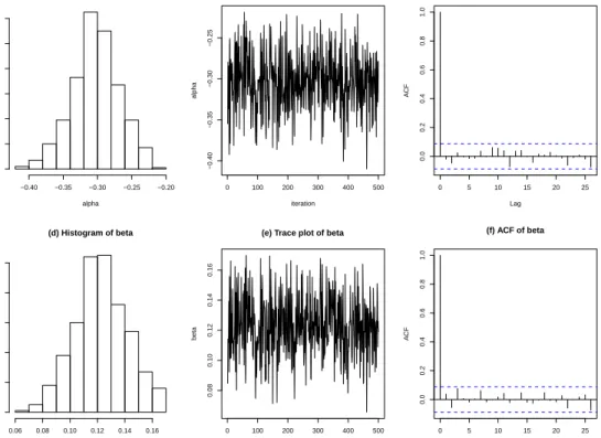
The remainder of this chapter is organized as follows. In Section B, we describe the BSAMC algorithm and explore its theoretical property. In Section C, we apply BSAMC to Ising models along with a comparison with the MCMLE algorithm. The numerical results show that BSAMC can perform very robustly to the initial guess of θ. In Section D, we apply BSAMC algorithm to autologistic and autonormal models.
B. Bayesian Stochastic Approximation Monte Carlo Algorithm 1. The BSAMC Algorithm
To approximate the normalizing constant κ(θ), the MCMLE method proposed by [32] adopts an importance sampling method with the trial distribution f(x|θ0). It is obvious that, when θ0 is far from the true value ofθ,f(x|θ0) may approximatef(x|θ) poorly, and the resulting estimate of κ(θ) may be biased. To resolve this difficulty, we choose the following mixture distribution as the trial distribution:
g(x, θ0) = 1 k k X i=1 p(x, θ0) ξ(i) I(x∈Ei), (4.1) where E1, . . . , Ek forms a partition of the sample space X, and ξ(i) =
R
Eip(x, θ0)dx.
Let ξ = (ξ(1), . . . , ξ(k)). Without loss of generality, we assume that the sample space has been partitioned according to the energy function −logp(x, θ0) as follows: E1 = {x : −logp(x, θ0) < h1}, E2 = {x : h1 ≤ −logp(x, θ0) < h2}, . . ., Ek = {x :
−logp(x, θ0) ≥ hk−1}, where h1 < h2 < . . . < hk−1 are some pre-fixed numbers. It is easy to see that sampling of g(x, θ0) will lead to an equal sampling from each of the subregions E1, . . . , Ek, and the normalizing constant κ(θ) can thus be well
approximated even when θ0 is far from the true value of θ. Clearly, the success of the approximation amounts on the estimation of the quantitiesξ(1), . . . , ξ(k)which are unknown a priori. Thanks to the SAMC algorithm, it provides consistent estimates
of these quantities in an iterative way. Let ξt(i) denote the estimate ofξ(i) at iteration t, letξt = (ξt(1), . . . , ξ (k) t ), and letx (1) t , . . . , x (m)
t denote the samples simulated from the
working trial distribution
gξt(x, θ0) = 1 Zt k X i=1 p(x, θ0) ξt(i) I(x∈Ei), (4.2) where Zt is the normalizing constant of gξt(x, θ0). Then logπ(θ|z) can be
approxi-mated by
logπξt(θ|z) = logπ(θ) + logp(z, θ)−log(Zt)−log
à 1 m m X i=1 p(x(ti), θ)/gξt(x (i) t , θ0) ! . (4.3) It is clear that as m→ ∞, logπξt(θ|z) approaches to logπ(θ|z).
BSAMC Algorithm
(a) (Auxiliary sample generating) Simulate samples x(1)t , . . . , x(tm) from the working trial distributiongξt−1(x, θ0) using the MH algorithm. Denote the set of auxiliary
samples by xt= (x(1)t , . . . , x(tm)).
(b) (Estimate updating) Update the estimatesξt−1 by setting
log (ξt) = log (ξt−1) +γtHξt−1(xt), (4.4)
where Hξt−1(xt) is a k-vector with the i-th component given by
Pm
j=1I(x (j)
t ∈
Ei)/m−1/k,I(·) is the indicator function, and{γt}is a pre-specified gain factor
sequence. How to choose the sequence {γt}will be discussed later.
(c) (Posterior sample generating) Draw sampleθ(1)t , . . . , θ(ts) from the approximated posterior πξt(θ|z) (as specified in (4.3)) using the MH algorithm.
Let (θ1(1), . . . , θ(1s)), . . ., (θn(1), . . . , θn(s)) denote the samples of θ generated in n
mean π(ϕ) = R ϕ(θ)π(θ|z)dθ can be estimated by \ πn(ϕ) = 1 (n−n0)s n X t=n0+1 s X i=1 ϕ(θt(i)), (4.5) where n0 denotes the burn-in time of the simulation. In Section 2, we show that under mild conditions, π\n(ϕ) converges almost surely to π(ϕ) when both n and m
become large.
The merit of this algorithm is the use of SAMC for learning of the trial distri-bution g(x, θ0). As discussed in [50], SAMC possesses a self-adjusting mechanism: If a component ξ(i) is underestimated (overestimated) in the current iteration, then the subregion Ei will tend to be oversampled (undersampled) in the next iteration and
the current estimate of ξ(i) will thus be counter-adjusted by the quantityγ
t(e(ti)−1/k)
as prescribed in step (b). This mechanism enables the simulation to converge very quickly with samples being drawn equally from different subregions of the sample space even when θ0 is far from the true value of θ. In general, the performance of BSAMC can be very robust to the choice of θ0.
For an effective implementation of BSAMC, several issues need to be considered: • Choice of θ0: Like the MCMLE method, θ0 can be chosen using another esti-mator of θ, which is easy to calculate, such as the maximum pseudo likelihood estimator (MPLE) [9] or the double MH estimator [48]. In our study, we set θ0 to the MPLE of θ.
• Sample space partition: As discussed in [50], the sample space should be par-titioned such that the simulation conducted in step (a) should have a reason-able acceptance rate. Since, within the same subregion, the SAMC simulation of gξt(x, θ0) is reduced to the MH simulation of f(x|θ0), the cutting values
prac-tice, we often set the subregions to have an equal energy bandwidth; that is, setting hi = hi−1 +δ with δ taking a value between 0 and 2. The value of h1 can be chosen to be reasonably small, and that of hk−1 can be reasonably large, such that both the energy regions of the true distribution f(x|θ) and of the initial distribution f(x|θ0) can be covered.
• Choice ofm: In practice, BSAMC is often run in two stages, although, in theory, this is not necessary. In stage I, a small value ofmis often used. The goal of this stage is to approximate ξi’s, so step (c) can be omitted in this stage. In stage
II, a large value of m is often used. The goal of this stage is draw samples of θ. This two-stage implementation strategy often improves the efficiency of the algorithm. In terms of MCMC simulations, stage I corresponds to the burn-in steps in (4.5).
• Choice of {γt}: As shown in [47], to ensure the convergence of ξt, {γt} should
be chosen as a positive, nondecreasing sequence satisfying the conditions (a) ¯limt→∞|γt−1−γt−1+1|<∞, (b) ∞ X t=1 γt =∞, and (c) ∞ X t=1 γtη <∞, (4.6) for some η >1. In this paper, we choose
γt=
t0 max(t0, t)
, t= 1,2,· · · (4.7)
for some specified value t0 > 1. As discussed in [50], a large value of t0 will force the sampler to reach all subregions quickly, even in the presence of multiple local energy minima. Therefore, t0 should be set to a large value for a complex problem. In practice, the choice oft0 should be associated with the choice ofN, the total number of iterations of the run. The appropriateness of their choices can be diagnosed by checking the convergence of multiple runs (starting with
different points) through an examination for the variation of ˆξ or ˆf, where ˆξ and ˆf denote, respectively, the estimate of ξ and the sampling frequencies of the subregions obtained at the end of a run. A rough examination for ˆξ is to see visually whether ˆξ’s produced in multiple runs follow the same pattern. Existence of different patterns implies that the gain factor is still large at the end of the runs or some parts of the sample space are not yet visited in all runs. This is similar to ˆf. If the choices of t0 andN are appropriate, each nonempty subregion should be sampled roughly equally at end of each run. If the runs are diagnosed as non-converged, BSAMC should be re-run with a large value of N, a larger value of t0, or both.
2. Convergence
For the reason of mathematical simplicity, we assume that Ξ, the parameter space of ξ, is compact. Therefore, the sequence{ξt}can be kept in a compact set. Extension of
our results to the case that Ξ = Rkis trivial with the technique of varying truncations
studied in [2] and [17], which ensures, almost surely, that the sequence {ξt} can be
kept in a compact set.
To establish the convergence of the BSAMC estimator (4.5), we first prove The-orem B.1, which concerns the convergence of ξt and the convergence of the sample
average of ρ(xt), where ρ denotes a bounded measurable function. Note that
Theo-rem B.1 concerns only steps (a) and (b) of BSAMC. If step (c) is ignored, BSAMC is reduced to the multiple SAMC algorithm studied in [47], where “multiple” means that multiple samples are allowed to be generated from the working density gξt(x|θ0)
at each iteration. Including step (c) enables BSAMC to be used for Bayesian in-ference for the models with intractable normalizing constants, and this is also the main methodology contribution of this paper. Rigorous theory has been established
for the methodology development. BSAMC also provides a general framework for approximated Bayesian analysis through sampling from a sequence of approximated distributions with their averages converging to the target posterior distribution.
With a slight abuse of notations, we let x = (x(1), . . . , x(m)) denote m MCMC samples drawn from g(x|θ0), and let g(x|θ0) denote the joint density/mass function of x. Then Theorem B.1 can be stated as follows:
Theorem B.1 Consider the BSAMC algorithm. If the condition (4.6) and the drift
condition (given in Appendix) hold and Ξ is compact, then for any integer m≥1, (i)
ξt(i) →cξi, a.s. as