Bootstrap inference for the finite population total under complex sampling designs

Statistics Publications Statistics

1-7-2019

Bootstrap inference for the finite population total

under complex sampling designs

Zhonglei Wang

Xiamen University

Jae Kwang Kim

Iowa State University, [email protected]

Liuhua Peng

The University of Melbourne

Follow this and additional works at:https://lib.dr.iastate.edu/stat_las_pubs

Part of theStatistical Methodology Commons, and theStatistical Theory Commons

The complete bibliographic information for this item can be found athttps://lib.dr.iastate.edu/ stat_las_pubs/255. For information on how to cite this item, please visithttp://lib.dr.iastate.edu/ howtocite.html.

This Article is brought to you for free and open access by the Statistics at Iowa State University Digital Repository. It has been accepted for inclusion in Statistics Publications by an authorized administrator of Iowa State University Digital Repository. For more information, please contact

Bootstrap inference for the finite population total under complex sampling

designs

Abstract

Bootstrap is a useful tool for making statistical inference, but it may provide erroneous results under complex survey sampling. Most studies about bootstrap-based inference are developed under simple random sampling and stratified random sampling. In this paper, we propose a unified bootstrap method applicable to some complex sampling designs, including Poisson sampling and probability-proportional-to-size sampling. Two main features of the proposed bootstrap method are that studentization is used to make inference, and the finite population is bootstrapped based on a multinomial distribution by incorporating the sampling information. We show that the proposed bootstrap method is second-order accurate using the Edgeworth expansion. Two simulation studies are conducted to compare the proposed bootstrap method with the Wald-type method, which is widely used in survey sampling. Results show that the proposed bootstrap method is better in terms of coverage rate especially when sample size is limited.

Disciplines

Statistical Methodology | Statistical Theory Comments

arXiv:1901.01645v1 [math.ST] 7 Jan 2019

Bootstrap inference for the finite population total under

complex sampling designs

Zhonglei Wang

_{Jae Kwang Kim}

_{Liuhua Peng}

Abstract

Bootstrap is a useful tool for making statistical inference, but it may provide er-roneous results under complex survey sampling. Most studies about bootstrap-based inference are developed under simple random sampling and stratified random sam-pling. In this paper, we propose a unified bootstrap method applicable to some com-plex sampling designs, including Poisson sampling and probability-proportional-to-size sampling. Two main features of the proposed bootstrap method are that studentiza-tion is used to make inference, and the finite populastudentiza-tion is bootstrapped based on a multinomial distribution by incorporating the sampling information. We show that the proposed bootstrap method is second-order accurate using the Edgeworth expansion. Two simulation studies are conducted to compare the proposed bootstrap method with the Wald-type method, which is widely used in survey sampling. Results show that the proposed bootstrap method is better in terms of coverage rate especially when sample size is limited.

Keywords: Confidence interval, Edgeworth expansion, Multinomial distribution, Second-order accurate.

∗_{Wang Yanan Institute for Studies in Economics and School of Economics, Xiamen University, Xiamen,}

Fujian 361005, P.R.C.

†_{Department of Statistics, Iowa State University, Ames, IA 50011, U.S.A.; Email: [email protected]} ‡_{School of Mathematics and Statistics, the University of Melbourne, Victoria 3010, Australia}

1

Introduction

Bootstrap, first proposed by Efron (1979), is a simulation-based approach for accessing uncertainty of estimates and for constructing confidence intervals. Bootstrap is widely used in that it is easy to implement and is second-order accurate under mild conditions (Hall;

1992, §3.3). However, classical bootstrap methods are not applicable under most sampling designs since the independent or identical distributed assumption may fail.

Under complex sampling, bootstrap methods have been proposed to handle variance es-timation. In survey sampling, one of the most popular bootstrap approaches is the rescaling bootstrap method proposed by Rao and Wu (1988) under stratified random sampling, and they demonstrated that their bootstrap-t intervals are second-order accurate if the variance component is known. Such a variance, however, is seldom known in practice. Rao et al.

(1992) generalized the rescaling bootstrap method to cover the non-smooth statistics, but they did not discuss the second-order accuracy. Sitter (1992a) considered a mirror-match bootstrap method for sampling designs without replacement and discussed the second-order accuracy based on the known population variance as Rao and Wu (1988). Sitter (1992b) extended the without-replacement bootstrap method (Gross;1980) to complex sampling de-signs and compared the proposed method with the rescaling bootstrap method (Rao and Wu;

1988) and the mirror-match bootstrap method (Sitter; 1992a). Shao and Sitter (1996) proposed a bootstrap method for the case when survey data are subject to missingness.

Sverchkov and Pfeffermann (2004) proposed to use a multinomial distribution to recon-struct the finite population to estimate the mean square error. Beaumont and Patak (2012) proposed a generalized bootstrap method for variance estimation under Poisson sampling.

Antal and Till´e (2011) proposed one-one resampling methods to estimate the variance for some complex sampling designs. Mashreghi et al. (2016) gave a comprehensive overview of the bootstrap methods in survey sampling for variance estimation.

In survey sampling, the literature on bootstrap-based approaches for interval estimation is very limited. Bickel and Freedman (1984) first considered interval estimation under

strat-ified random sampling. Booth et al. (1994) generalized the method of Bickel and Freedman

(1984) to show that the constructed confidence interval for a smooth function of the finite population mean is second-order accurate. However, all of the theoretical results, includ-ing that of Rao and Wu (1988) are restricted to stratified random sampling. Although

Beaumont and Patak (2012) discussed a generalized bootstrap method for survey sampling with special attention to Poisson sampling, they did not provide rigorous results for the second-order accuracy of their methods.

In this paper, we focus on interval estimation under complex sampling. The goal of this study is to develop a unified bootstrap method to approximate the sampling distribution of the design-based estimator under some popular sampling designs, including Poisson sam-pling, simple random sampling (SRS) and probability-proportional-to-size (PPS) sampling. The proposed bootstrap methods apply multinomial distributions to generate the bootstrap finite populations by incorporating the sampling information, and the same sampling design is conducted to obtain a bootstrap sample from each bootstrap finite population. A similar idea has been successfully applied to SRS by Gross (1980) and Chao and Lo (1985). Our bootstrap methods differ from that proposed by Sverchkov and Pfeffermann (2004) in the sense that the finite population is iteratively bootstrapped, and an asymptotically pivotal statistic is used to make statistical inference for the finite population total. We also study the theoretical properties of the proposed bootstrap methods for different sampling designs using the Edgeworth expansion. We summarize our contributions in this paper below:

1. We have proposed a unified bootstrap method for interval estimation under some pop-ular complex sampling designs, including Poisson sampling, SRS and PPS sampling. A simulation study also confirms that the proposed method works even under two-stage cluster sampling.

2. For three commonly used sampling designs, we have provided a rigorous proof for the second-order accuracy of the proposed bootstrap methods and shown that the estima-tion error isoppn´1{2q(DiCiccio and Romano;1995) under mild conditions. Wald-type

method is widely used in survey sampling, so the proposed bootstrap method is an important contribution since it provides more accurate inference compared with the Wald-type method under mild conditions. Besides, to our knowledge, we are the first to provide the Edgeworth expansion of astudentized estimator under Poisson sampling. The remaining part of the paper is organized as follows. Sampling designs and design-based estimators under consideration are briefly reviewed in Section 2. In the following three sections, we propose bootstrap methods for Poisson sampling, SRS and PPS sampling, respectively, and theoretical properties are also investigated. Two simulation studies are conducted to compare the proposed bootstrap method with the Wald-type method in Section 6. Some concluding remarks are made in Section 7.

2

Sampling designs and estimates

In survey sampling, the finite population is often assumed to be fixed, and the randomness is due to the sampling design. Let FN “ ty1, . . . , yNu be the finite population of size N,

and we are interested in making inference for the finite population total Y _“ řN

i“1yi. For

simplicity, we assume that the elements in FN are scalers. To avoid unnecessary details,

we also assume that the population size N is known, so it is equivalent to make statistical inference for the finite population mean ¯Y _“N´1_Y.

We consider three commonly used sampling designs, including Poisson sampling, SRS and PPS sampling. For without-replacement sampling designs, such as Poisson sampling and SRS, Ii is the sampling indicator with Ii “1 indicating that the i-th element is in the

sample and 0 otherwise, and πi “ EpIiq is the first-order inclusion probability of the i-th

element fori_“1, . . . , N, where the expectation is taken with respect to the sampling design. Let ΠN “ tπ1, . . . , πNube the set of first-order inclusion probabilities, and it is assumed to be

known. Poisson sampling generates a sample based onN independent Bernoulli experiments, one for each element in the finite population. That is, Ii „ Berpπiq for i “ 1, . . . , N,

where Berpπiq is a Bernoulli distribution with success probability πi P p0,1q, and a sample

is _tyi : Ii “ 1, i “ 1, . . . , Nu. Let n “ ř N

i“1Ii be a realized sample size and n0 “ Epnq “ řN

i“1πibe the expected sample size under Poisson sampling. For SRS, a without-replacement

sample of size n is selected with equal probabilities, and we can show πi “ nN´1 for i “

1, . . . , N under SRS. Denote ˆYP oi “

řN

i“1yiπi´1Ii to be the Horvitz-Thompson estimator

(Horvitz and Thompson; 1952) of Y under Poisson sampling, and the corresponding one is ˆYSRS “ řN_i“1yiπ´i 1Ii “ N n´1řN_i“1Iiyi under SRS. The sample size n is random under

Poisson sampling, but it is fixed under SRS. Without loss of generality, assume that the first

n elements are sampled under Poisson sampling or SRS, and the design-unbiased variance estimators are ˆVP oi “

řn

i“1yi2p1´πiqπi´2 and ˆVSRS “NpN´nqn´1s2SRS, respectively, where s2

SRS “n´1

řn

i“1pyi´y¯q2 is the sample variance ofty1, . . . , ynu, and ¯y“n´1

řn

i“1yi.

PPS sampling generates a sample of size n by independently and identically selecting an element from FN n times with selection probabilitiestpi :i“1, . . . , Nu, where pi P p0,1qis

the knownselection probability of yi fori“1, . . . , N and řN_i“1pi “1. Replicates may occur

in the sample under PPS sampling, and the population totalY is estimated by the Hansen– Hurwitz estimator (Hansen and Hurwitz; 1943), which is denoted as ˆYP P S “ n´1řn_i“1Zi,

whereZi “p´a,i1ya,i,pa,i“pkandya,i“ykifai “k, andaiis the index of the selected element

for the i-th draw. A design-unbiased variance estimator is ˆVP P S “n´2

řn

i“1pZi´YˆP P Sq2.

Throughout the paper, assume that the (expected) sample size is less than the population size. Since we study a sequence of finite populations and inclusion probabilities in the following three sections, assume thatyi and πi are indexed by N implicitly, and samples are

generated independently for different finite populations. We use the notation “an —bn” to

indicate that an and bn have the same asymptotic order. That is, an —bn is equivalent to an “Opbnq and bn “Opanq.

3

Bootstrap method for Poisson sampling

We propose the following bootstrap method to approximate the sampling distribution of

TP oi “Vˆ

´1{2

P oi pYˆP oi´Yq under Poisson sampling.

Step 1. Based on the sample _ty1, . . . , ynu, generate pN1˚, . . . , Nn˚q from a multinomial

distri-bution MN_pN;ρ_q with N trials and a probability vector ρ, where ρ _{“ p}ρ1,¨ ¨ ¨ , ρnq

and ρi “ πi´1 řn j“1π ´1 j for i _“1, . . . , n. Denote F˚

N “ ty1˚, . . . , yN˚u and Π˚N “ tπ˚1, . . . , πN˚u, and they consist

of Ni˚ copies of yi and πi, respectively. Let the bootstrap finite population total be

Y˚ _“řN

i“1yi˚ “

řn

i“1Ni˚yi.

Step 2. For i_“1,_{¨ ¨ ¨}, n, generate m˚

i independently from a binomial distribution BinpNi˚, πiq

with N_i˚ trials and a success probability πi. The bootstrap sample consists of m˚i

replicates of yi under Poisson sampling. Denote ˆYP oi˚ “

řn i“1m ˚ iyiπi´1 and TP oi˚ “ pVˆ_{P oi}˚ _q´1{2_pYˆ˚ P oi ´Y˚q, where ˆVP oi˚ “ řn

i“1m˚iy2ip1´πiqπi´2 is the bootstrap variance

estimator.

Step 3. Repeat the two steps above independently M times.

Step 1 corresponds to generating a bootstrap finite population F˚

N and bootstrap

first-order inclusion probabilities Π˚

N by incorporating the sampling information. Based on FN˚

and Π˚

N, Step 2 is used to generate a bootstrap sample, from which a bootstrap replicate of TP oi is obtained. Instead of sampling from the bootstrap finite populationFN˚ directly, Step 2

provides a more efficient way to generate a sample usingN₁˚, . . . , N_n˚under Poisson sampling. In Step 2, we center TP oi˚ by the bootstrap population total Y˚ not by ˆYP oi. The reason is

that the finite population should be fixed, and the randomness is due to Poisson sampling. Thus, the statistic should be centered using the corresponding population total Y˚_{. If we} center T˚

finite populations. The same argument applies for the other two sampling designs. We use the empirical distribution of T_{P oi}˚ to approximate that of TP oi and make inference for Y.

Before discussing the theoretical properties of the proposed bootstrap method, we intro-duce some mild conditions onFN and ΠN.

(C1) There exist constantsα_{P p}2´1_{,1sand 0ăC}

1 ďC2 such thatn0 —Nα, andπi satisfies C1ďn0´1N πi ďC2

for i_“1, . . . , N.

(C2) The sequence of finite populations and first-order inclusion probabilities satisfy lim NÑ8pn0N ´2_V P oiq “σ21, where VP oi “ řN

i“1yi2p1´πiqπi´1, and σ12 is a positive constant.

(C3) The following condition holds for finite populations, that is, lim NÑ8N ´1 N ÿ i“1 y_i8 _“C3,

where C3 is a positive constant.

(C4) Denote Xi “ V´

1{2

P oi yiπ

´1

i pIi´πiq for i “ 1, . . . , N, and let m “ tn´

1{2

0 N{plogn0qu be

the integer part ofn´₀1{2N_{plogn0q. Then, there exist constants t0 ą0 andaą2 such

that, for any subset _tXℓ1, . . . , Xℓmuof tX1, . . . , XNu,

ˇ ˇ ˇ ˇ ˇ m ź i“1 E_texp_pιtXℓiq |FNu ˇ ˇ ˇ ˇ ˇ “O_pm´a_q

uniformly in_|t_{| ą}t0 ą0, where ι is the imaginary unit.

sampling (Fuller; 2009); the first part of (C1) is a mild restriction on the expected sample size, and the second part regulates the first-order inclusion probabilities. Condition (C2) rules out the degenerate case of the Horvitz–Thompson estimator under Poisson sampling. The moment condition in (C3) guarantees the convergence of the variance estimators and other quantities, and it is also required for SRS and PPS sampling that we will discuss in the following two sections. To illustrate the existence of FN and ΠN satisfying (C1) and (C2)

simultaneously, consider πi “ n0N´1, so (C1) holds, where n0 “ tN2{3u and C1 “ C2 “ 1,

for example. Then, we have limNÑ8pn0N´2VP oiq “ limNÑ8N´1řNi“1y 2

i p1´n0N´1q. If

N´1řN

i“1y 2

i converges as N Ñ 8, then (C2) holds. Condition (C4) is a counterpart of

non-lattice assumption and is useful in deriving Edgeworth expansions. Specifically, for any subset _tXℓ1, . . . , Xℓmu of tX1, . . . , XNu, condition (C4) ensures that tXℓiu

m

i“1 have

subse-quences of length O_plogm_q with different spans; see Feller (2008,§16.6) for more discussion on a similar assumption.

Denote _pFN,BN, PN,P oiq to be a probability space, where BN and PN,P oip¨q are the σ

-algebra and the probability measure on FN associated with Poisson sampling, respectively.

That is, FN “ ŚN_i“1Ωi, BN “ ÂN_i“1Ai and PN,P oipA1 ˆA2 ˆ ¨ ¨ ¨ ˆANq “ śN_i“1µipAiq,

where Ωi “ t0,1u,Ai is the power set of Ωi, andµipt1uq “1´µipt0uq “ πi for i“1, . . . , N.

Let F _“ Ś8

N“1FN be the product space and B “

Â8

N“1BN be the product-σ-algebra;

see Klenke (2014, §14.1) for details about the notations. By Corollary 14.33 of Klenke

(2014), there exists a uniquely determined probability measure P_{P oi on pF,Bq such that} P_{P oipF1 ˆF2 ˆ ¨ ¨ ¨ ˆFnˆ}Ś8

N“n`1FNq “ śn

i“1Pi,P oi, where Fi P Fi for i “ 1, . . . , n and

n_P N_.

Lemma 3.1. Suppose that (C1)–(C3) hold. Then,

n0N´2pVˆP oi´VP oiq Ñ 0 (1)

Letµp_{P oi}3q _“řN i“1y 3 ip1´πiqtp1´πiq2πi´2´1uandµˆ p3q P oi “ řn i“1y 3 ip1´πiqπi´1tp1´πiq2πi´2´1u. Then, n₀2N´3µ_{P oi}p3q _“O_p1_q and n 2 0 N3pµˆ p3q P oi´µ p3q P oiq “Oppn´ 1{2 0 q. (2) In addition, denote τ_{P oi}p3q _“řN i“1y 3 ip1´πiq2πi´2 and τˆ p3q P oi “ řn i“1y 3 ip1´πiq2πi´3. Then, n2 0 N3τ p3q P oi “Op1q and n2 0 N3pτˆ p3q P oi´τ p3q P oiq “ Oppn ´1{2 0 q. (3)

Lemma 3.1 shows some basic properties of the finite population quantities and their design-based estimators. Specifically, the ratio ˆV_{P oi}´1VP oi Ñ 1 almost surely pPP oiq by (C2).

Under Poisson sampling, µp_{P oi}3q is the third central moment of ˆYP oi, and τp

3q

P oi is a quantity

involved in the Edgeworth expansion of the distribution of TP oi.

Theorem 3.1. Assume that conditions (C1)–(C4) hold. Let FˆP oipzq “ PP oipTP oi ďzq be the cumulative distribution function of TP oi under Poisson sampling. Then,

ˆ µp_{P oi}3q ˆ V_{P oi}3{2 “Oppn ´1{2 0 q and ˆ τ_{N,P oi}p3q ˆ V_{N,P oi}3{2 “Oppn ´1{2 0 q. (4) Furthermore, ˆ FP oipzq “Φpzq ` # ˆ µp<sub>N,P oi</sub>3q 6 ˆV<sub>N,P oi</sub>3{2 p1´z 2 q ` τˆ p3q N,P oi 2 ˆV_{N,P oi}3{2 z 2 + φ_pz_{q `}oppn´ 1{2 0 q (5)

uniformly inz _PR_{, whereΦpzqis the cumulative distribution function of the standard normal} distribution with the probability density function φ_pz_q.

we make brief comments on the opp¨q notation in (5) of Theorem 3.1. The probability

ˆ

FP oipzq on the left side of (5) is not random. However, we use estimators in the Edgeworth

expansion to make it easier to compare (5) with the result in the following theorem, so instead of o_p¨q, it is reasonable to use opp¨qon the right side of (5). Similar argument can be

In order to establish the Edgeworth expansion for the conditional distribution of T_{P oi}˚ , we need the following assumption, which is similar to condition (C4) but with m replaced by n0. We isolate (C4) and (C5) since (C5) is not needed for Theorem 3.1.

(C5) There exist constants t0 ą 0 and a ą 2 such that, for any subset tXℓ1, . . . , Xℓn0u of

tX1, . . . , XNu with cardinality n0, ˇ ˇ ˇ ˇ ˇ n0 ź i“1 E_texp_pιtXℓiq |FNu ˇ ˇ ˇ ˇ ˇ “O_pn´0aq uniformly in_|t_{| ą}t0 ą0.

The next theorem presents the Edgeworth expansion for the distribution of T˚

P oi based

on the proposed bootstrap method.

Theorem 3.2. Suppose that conditions (C1)–(C5) hold. Let Fˆ_{P oi}˚ _pz_q be the cumulative dis-tribution function of T_{P oi}˚ conditional on the bootstrap finite populationF˚

P oi. Then, ˆ F_{P oi}˚ _pz_{q “}Φ_pz<sub>q `</sub> # ˆ µp<sub>N,P oi</sub>3q 6 ˆV<sub>N,P oi</sub>3{2 p1´z 2 q ` τˆ p3q N,P oi 2 ˆV_{N,P oi}3{2 z 2 + φ_pz_{q `}oppn´ 1{2 0 q (6) uniformly in z _PR_.

By comparing (5) in Theorem 3.1 with (6) in Theorem 3.2, we show that the proposed bootstrap method is second-order accurate, but the Wald-type method, which is based on the asymptotic normality of TP oi, is not if µp

3q

P oi and τ

p3q

P oi are nonzero by noting the fact that

ˆ

µp_{P oi}3q and ˆτ_{P oi}p3q are design-unbiased estimators of µp_{P oi}3q and τ_{P oi}p3q, respectively. Typically, the cumulative distribution function ˆF_{P oi}˚ _pz_qis hard to study analytically, so we use an empirical distribution to approximate it.

Now, consider establishing confidence intervals for the population total Y. An approx-imate two-sided confidence interval at significance level α based on the Wald-type method

can be constructed as ´ ˆ YP oi´q1´α{2Vˆ 1{2 P oi,YˆP oi´qα{2Vˆ 1{2 P oi ¯ , (7)

whereqα{2 and q1´α{2 are the pα{2q andp1´α{2q quantiles of the standard normal

distribu-tion, respectively. According to Theorem 3.1, though the upper and lower confidence limits of (7) have error rates of order Oppn

´1{2

0 q, this two-sided confidence interval has error rate

of order oppn´1{2q since ˆµ p3q N,P oi{p6 ˆV 3{2 N,P oiqp1´z 2 q `τˆ_{N,P oi}p3q _p2 ˆV_{N,P oi}3{2 _qz2 is an even function ofz, and the n´01{2 order term in the Edgeworth expansion ofTP oi cancel in the error rate.

How-ever, then´01{2 order term leads to an error rates of orderOppn´01{2qfor one-sided confidence

intervals based on the normal approximation.

The confidence interval of Y based on the proposed bootstrap methods is

´ ˆ YP oi´q˚1´α{2Vˆ 1{2 P oi,YˆP oi´qα˚{2Vˆ 1{2 P oi ¯ , (8) where q˚

α{2 and q˚1´α{2 are the pα{2q and p1´α{2q quantiles of ˆFP oi˚ pzq. By Theorem 3.2,

the coverage error of (8) is of order oppn´

1{2

0 q. Moreover, the upper and lower limits of (8)

have error ratesoppn´

1{2

0 q, which outperforms the confidence interval (7) based on Wald-type

method. In addition, the one-sided confidence interval by the proposed bootstrap method is more accurate than the one-sided confidence interval obtained by the Wald-type method. Furthermore, as discussed in Section 3.6 ofHall(1992), an asymmetric equal-tailed confidence interval may convey important information. The same arguments can be used for the other two sampling designs.

4

Bootstrap method for SRS

We propose the following procedure to make statistical inference forTSRS “Vˆ_SRS´1{2pYˆSRS´Yq

Step 1. Generate pN₁˚, . . . , N_n˚_q from MNpN;ρ_q, where ρi “ n´1 for i “ 1, . . . , n. Then, FN˚

contains N_i˚ copies of yi for i “1, . . . , n, and the bootstrap finite population total is

Y˚ _“řN

i“1Ni˚yi.

Step 2. Generate a bootstrap sample of size n, denoted as _ty1˚, . . . , y˚nu, from FN˚ using SRS.

Then, we can obtain TSRS˚ “ pVˆSRS˚ q´1{2pYˆSRS˚ ´Y˚q, where ˆYSRS˚ “ N n´1

řn i“1y˚i, ˆ V˚ SRS “NpN ´nqn´1sSRS˚2 ,s˚SRS2 “n´1 řn i“1pyi˚´y¯˚q2, and ¯y˚ “n´1 řn i“1y˚i.

Step 3. Repeat the two steps above independently M times.

The three steps for SRS are similar to those under Poisson sampling, but we do not need Π˚

N since πi˚ “ nN´1 for i “ 1, . . . , N. Different from that under Poisson sampling, the

bootstrap sample is generated directly fromF˚

N. One commonly used algorithm to generate

a sample of size n under SRS is to select elements sequentially from the finite population without replacement. Ifn _“o_pN_q, the computational complexity of selecting each element is

O_pN_q. Besides the above bootstrap procedure, we propose the following one. It can be shown that these two procedures are equivalent under SRS, but the computational complexity of the latter is O_pn_q for selecting each element.

Step 1’. The same as Step 1 above.

Step 2’. Initialize N_i˚p0q _“Ni˚ and m˚i “0 for i“1, . . . , n.

Step 3’. Generate a bootstrap sample of size n from F˚

N under SRS.

Step 3.1’. Initialize k _“1.

Step 3.2’. Select an index, saylpkq, from_t1, . . . , n_uwith selection probabilityppikq“N

˚pk´1q i { řn j“1N ˚pk´1q j for i_“1, . . . , n.

Step 3.3’. Update m˚i “ m˚i `1 if i “lpkq. Set N

˚pkq i “N ˚pk´1q i if i P t1, . . . , nuztlpkqu, and Ni˚pkq “N ˚pk´1q

i ´1 if i “lpkq, where AzB “ txP A: xR Bu for two sets A and B.

Step 3.4’. Set k_“k_`1, and go back to Step 3.2’ until k_ąn. Step 3.5’. Obtain T˚ SRS “ pVˆSRS˚ q´1{2pYˆSRS˚ ´Y˚q, where ˆYSRS˚ “ N n´1 řn i“1m˚iyi, ˆVSRS˚ “ N_pN _´n_qn´1_s˚2 SRS, s˚SRS2 “n´1 řn i“1m˚ipyi´y¯˚q2, and ¯y˚ “n´1řn_i“1m˚iyi.

Step 4’. Repeat the above three steps independently M times.

We list some necessary conditions for studying the theoretical properties of the proposed bootstrap method under SRS.

(C6) There exist β _{P p}2´1_,1

sandκ_{P p}0,1_qsuch thatn _—Nβ _{and nN}´1

ď1_´κasN _{Ñ 8}.

(C7) The finite population satisfies

lim NÑ8σ 2 SRS “σ22, where σ2SRS “N´1 řN

i“1pyi´N´1Yq2, andσ22 is a positive constant.

(C8) The distribution GN,SRS converges weakly to a strongly non-lattice distribution GSRS,

where GN,SRS assigns probability 1{N to y1, . . . , yN.

Condition (C6) is a counterpart of (C1), and it is used to rule out the trivial case when the sample size equals to that of the finite population. Condition (C7) regulates the variance of FN with respect to the distribution GN,SRS, and it concentrates our discussion on the

non-degenerate case under SRS. The non-latticed assumption in (C8) is used to make the discussion easier, and a distribution G_px_q is strongly non-latticed if |ş

exp_pιtx_qdG_px_q| _‰ 1 for all t_‰0; see Babu and Singh (1984) for details.

We can use a similar argument made in Section 3 to show that there exists a probability measure P_{SRS on the product space F “}Ś8

N“1FN equipped with the productσ-algebraB.

Lemma 4.1. Suppose that (C3), (C6) and (C7) hold. Then,

where µp_SRS3q _“N´1řN

i“1pyi´N´ 1_Y

q3 _{is the third central moment of F}

N with respect to the distribution GN,SRS. Besides,

s2_SRS´σ2_{SRS Ñ}0 (10)

as N _{Ñ 8} almost surely _pP_{SRSq. In addition,}

ˆ

µ_SRSp3q _´µ_SRSp3q _“opp1q, (11)

where µˆp_SRS3q _“n´1řn

i“1y 3

i `2¯y3n´3¯ynn´1řn_i“1yi2, and y¯n“n´1řn_i“1yi is the sample mean.

Lemma 4.1 is the counterpart of Lemma 3.1 under SRS, and it shows the convergence properties of the sample variance and third central moment under mild conditions. We do not use scaling factors in (9)–(11) since the quantities involved are with respect to the distribution GN,SRS.

Theorem 4.1. Suppose that (C3) and (C6)–(C8) hold. Then,

ˆ FSRSpzq “Φpzq `p 1<sub>´</sub>n<sub>{</sub>N<sub>q</sub>1{2µˆp<sub>SRS</sub>3q 6n1{2<sub>s</sub>3 SRS " 3z2<sub>´</sub>1´2n{N 1´n<sub>{</sub>N pz 2 ´1<sub>q</sub> * φ<sub>p</sub>z<sub>q `</sub>oppn´1{2q (12) uniformly inz _PR_{, whereF}ˆ_{SRSpzq “}P_{SRSpTSRS ďzqis the cumulative distribution function} of TSRS.

Theorem 4.1shows the Edgeworth expansion for the distribution of TSRS, and this result

is obtained by one result in Section 2 ofBabu and Singh (1985). Instead of using µp_SRS3q and

σSRS as done by Babu and Singh (1985), we use their estimators in (12) based on Lemma

4.1.

Theorem 4.2. Suppose that (C3) and (C6)–(C8) hold. Then, we have

ˆ F_SRS˚ _pz_{q “}Φ_pz_{q `</sub>p1´n{Nq 1{2<sub>µˆ</sub>p3q SRS 6n1{2<sub>s</sub>3 SRS " 3z2<sub>´</sub>1´2n{N 1´n<sub>{</sub>N pz 2 ´1<sub>q</sub> * φ<sub>p</sub>z<sub>q `}oppn´1{2q (13)

uniformly inz _PR_{, whereF}ˆ_SRS˚ _{pzqis the cumulative distribution function ofTSRS}˚ _conditional on the bootstrap finite population F˚

N.

Theorem 4.2 shows the Edgeworth expansion for the distribution of T_SRS˚ obtained by the proposed bootstrap method. By comparing (12) in Theorem 4.1 with (13) in Theorem

4.2, we have shown the second-order accuracy of the proposed bootstrap method.

5

Bootstrap method for PPS sampling

We consider PPS sampling in this section and propose the following bootstrap method to approximate the sampling distribution of TP P S “Vˆ_{P P S}´1{2pYˆP P S´Yq.

Step 1. ObtainpN_a,˚₁, . . . , N_a,n˚ _qfrom a multinomial distribution MNpN;ρ_q, whereρ_{“ p}ρ1, . . . , ρnq

and ρi “ p´a,i1p

řn

j“1p

´1

a,jq´1 for i “ 1, . . . , n. Then, FN˚ “ ty˚1, . . . , yN˚u consists of N_a,i˚ copies of ya,i, and the bootstrap finite population total is Y˚ “ ř

N

i“1yi˚ “

řn

i“1Na,i˚ ya,i. The bootstrap selection probabilities are tpCN˚q´1p˚1, . . . ,pCN˚q´1p˚Nu,

where CN˚ “

řN

i“1p˚i “

řn

i“1Na,i˚ pa,i, and tp1˚, . . . , p˚Nu consists of Na,i˚ copies of pa,i

for i_“1, . . . , n. Step 2. Based onF˚

N, generate a sample of sizenby independently and identically selecting an

element fromF˚

N n times with selection probabilitiestpCN˚q´1p˚i :i“1, . . . , Nu. Then,

we have T_{P P S}˚ _{“ p}Vˆ_{P P S}˚ _q´1{2_pYˆ˚

P P S´Y˚q, where ˆYP P S˚ “n´1

řn

i“1C

˚

Npp˚b,iq´1y˚b,i , yb,i˚ “ y˚_k andp˚_{b,i “}p˚_k if the index of thei-th draw isk, and ˆV_{P P S}˚ _“n´2řn

i“1tC

˚

Npp˚b,iq´1yb,i˚ ´

ˆ

Y_{P P S}˚ _u2 _{is the counterpart of ˆV}

P P S based on the bootstrap sample.

Step 3. Repeat the two steps above independently M times.

To implement the proposed bootstrap method for PPS sampling, the bootstrap selection probability should be standardized before drawing a sample. Similarly to the previous two sections, we use the empirical distribution of T˚

The computational complexity of selecting an element in Step 2 is O_pN_q. An equivalent way of carrying out the proposed bootstrap method under PPS sampling is described below, and its computational complexity is O_pn_qfor selecting an element.

Step 1’. The same as Step 1 above.

Step 2’. Obtain an independent and identical sample of sizenfrom_t1, . . . , n_u, and the selection probability of i is p:_{i “ p}C_N˚_q´1_N˚

i pa,i for i “ 1, . . . , n. Denote m˚i to be the number

of i’s in the sample. Then, we have T_{P P S}˚ _{“ p}Vˆ_{P P S}˚ _q´1{2_pYˆ˚

P P S´Y˚q, where ˆVP P S˚ “ n´2řn

i“1m˚ipCN˚p´a,i1ya,i´YˆP P S˚ q2 and ˆYP P S˚ “n´1

řn

i“1m˚iCN˚p´a,i1ya,i.

Step 3’. Repeat the above three steps independently M times.

The following regularity conditions are required to validate the proposed bootstrap method under PPS sampling.

(C9) There exists γ _{P p}2´1_{,1ssuch that n —N}γ_{, and the selection probabilities satisfy} C4 ďN pi ďC5

for i_“1, . . . , N, where C4 and C5 are positive constants.

(C10) The sequence of finite populations and selection probabilities satisfy lim NÑ8pN ´2_σ2 P P Sq “σ23, where σ2 P P S“ řN i“1pipp ´1

i yi´Yq2, and σ32 is a positive number.

(C11) The distribution GN,P P S is non-lattice, where GN,P P S assigns probability pi to p´i 1yi

for i_“1, . . . , N.

Condition (C9) regulates the sample size and selection probabilities, and (C10) rules out the degenerate case under PPS sampling. To show (C9) and (C10) can be satisfied

simultaneously, take pi “ N´1 for i “ 1, . . . , N. Then, (C9) holds with 0 ă C4 ă1 ă C5, andσ2 P P S “ řN i“1pipp ´1 i yi´Yq2 “Nř N i“1y 2 i ´N2Y¯2, where ¯Y “N´1Y. Thus, N´2σP P S2 “ N´1řN i“1yi2´Y¯2 converges if both N´1 řN

i“1y2i and ¯Y converge as N Ñ 8. Since GN,P P S

corresponds to the PPS sampling procedure, condition (C11) focuses our attention to the non-lattice case.

Based on a similar argument made under Poisson sampling, there exists a probability measure P_{P P S on F “} Ś8

N“1FN equipped with the product σ-algebra B under PPS

sam-pling.

Lemma 5.1. Suppose that (C3), (C9) and (C10) hold. Then,

N´2_ps2_{P P S´}σ_{P P S}2 _{q Ñ}0 (14)

as N _{Ñ 8} almost surely _pP_{P P Sq, where s}2

P P S “ n´1

řn

i“1pZi ´Z¯nq2 is the sample vari-ance of _tZ1, . . . , Znu. Let µ p3q P P S “ řN i“1pippi´1yi ´Yq3 and µˆ p3q P P S “ n´ 1řn i“1Z 3 i `2 ¯Zn3 ´ 3 ¯Znn´1 řn i“1Z 2 i, then N´3µp_{P P S}3q _“O_p1_q and N´3_pµˆ_{P P S}p3q _´µp_{P P S}3q _{q “}Oppn´1{2q. (15)

Lemma 5.1 shows convergence properties of estimators of the variance and third central moment. The next theorem deals with the Edgeworth expansion for the distribution ofTP P S. Theorem 5.1. Suppose that (C3), (C9)–(C11) hold. Then,

ˆ FP P Spzq “Φpzq ` ˆ µp<sub>P P S</sub>3q 6?ns3 P P S p2z2 <sub>`</sub>1_qφ_pz_{q `}oppn´1{2q (16) uniformly in z _P R_{, where F}ˆ_{P P S “} P_{P P SpTP P S ďzq is the cumulative distribution function} of TP P S under PPS sampling.

Based on the result in Theorem 5.1, the Wald-type method may provide inefficient infer-ence results for Y compared with the proposed bootstrap method if the sample size is small

and µp_{P P S}3q _‰0.

Theorem 5.2. Suppose that (C3), (C9)–(C11) hold. Then, we have

ˆ FP P S˚ pzq “Φpzq ` ˆ µp<sub>P P S</sub>3q 6?ns3 P P S p2z2 <sub>`</sub>1_qφ_pz_{q `}oppn´1{2q (17) uniformly inz _PR_{, whereF}ˆ_{P P S}˚ _{pzqis the cumulative distribution function ofTP P S}˚ _conditional on the bootstrap finite population FN˚.

Theorem 5.2 shows the Edgeworth expansion for the cumulative distribution function of

T_{P P S}˚ based on the proposed bootstrap method. By comparing (16) in Theorem 5.1 with (17) in Theorem 5.2, we have shown that the proposed bootstrap method is second-order accurate under PPS sampling.

6

Simulation study

6.1

Single-stage sampling designs

We conduct a simulation study based on single-stage sampling designs in this section. A finite population FN “ ty1, . . . , yNu is generated by

yi „Expp10q

for i _“ 1, . . . , N, where Exp_pλ_q is an exponential distribution with a scale parameter λ, and the population size is N _“ 500, which is assumed to be known. The size measure is simulated byzi “logp3`siqfori“1, . . . , N, where si |yi „Exppyiq. The expected sample

size is n0 P t10,100u. We are interested in constructing a 90% confidence interval for the

finite population mean ¯Y by survey data under the following sampling designs, and its true value is around 9.7.

1. Poisson sampling. The first-order inclusion probability is πi “ n0zi ´ řN j“1zj ¯´1 for

i_“1, . . . , N, and its expected sample size is n0.

2. SRS with sample size n0.

3. PPS sampling. The selection probability for this design is pi “ zi

´ řN

j“1zj ¯´1

for

i_“1, . . . , N, and the sample size isn0.

Based on a sample, denote ˜V to be the design-unbiased variance estimator of ˜Y, where ˜

Y is the design-unbiased estimate of ¯Y under a specific sampling design. We consider the following methods to construct the 90% confidence interval.

Method I. Proposed bootstrap method by settingM _“1 000. DenoteqB,0.05 andqB,0.95 to be the

5%-th and 95%-th sample quantiles of _tpV˜˚pmq_q´1{2

pY˜˚pmq _´Y¯˚pmq_{q : m “ 1, . . . , Mu} obtained by the proposed bootstrap method, where ˜V˚pmq_{, ˜Y}˚pmq _{and ¯Y}˚pmq _{are the} bootstrap counterparts of ˜V, ˜Y and ¯Y in the m-th repetition. Then, a 90% confidence interval for ¯Y can be constructed by

pY˜ _´qB,0.95V˜1{2,Y˜ ´qB,0.05V˜1{2q.

Method II. Wald-type method. A Wald-type 90% confidence interval for ¯Y is obtained by

pY˜ _´q0.95V˜1{2,Y˜ ´q0.05V˜1{2q,

where q0.05 and q0.95 are the 5%-th and 95%-th quantiles of the standard normal

dis-tribution.

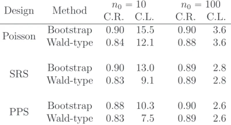
We conduct 1 000 Monte Carlo simulations for each sampling design, and the two methods are compared in terms of the coverage rate and the length of the constructed 90% confidence interval. Table 1 summarizes the simulation results. When the sample size is small, the proposed bootstrap method is more preferable in the sense that its coverage rates are closer to

Table 1: Coverage rate and length of the constructed 90% confidence interval for the proposed bootstrap method (Bootstrap) and the Wald-type method (Wald-type) under single-stage sampling designs, including Poisson sampling (Poisson), SRS and PPS sampling (PPS). “C.R.” stands for the coverage rate, and “C.L.” presents the Monte Carlo mean of the lengths of the constructed confidence interval.

Design Method n0 “10 n0 “100 C.R. C.L. C.R. C.L. Poisson Bootstrap 0.90 15.5 0.90 3.6 Wald-type 0.84 12.1 0.88 3.6 SRS Bootstrap 0.90 13.0 0.89 2.8 Wald-type 0.83 9.1 0.89 2.8 PPS Bootstrap 0.88 10.3 0.90 2.6 Wald-type 0.83 7.5 0.89 2.6

0.9 compared with the Wald-type method under the three sampling designs. The confidence interval constructed by the proposed bootstrap method is wider compared with that by the Wald-type method. As the sample size increases to n0 “ 100, the performance of the two

methods is approximately the same in the sense that the coverage rates of both methods are close to 0.9, and confidence interval lengths are approximately the same.

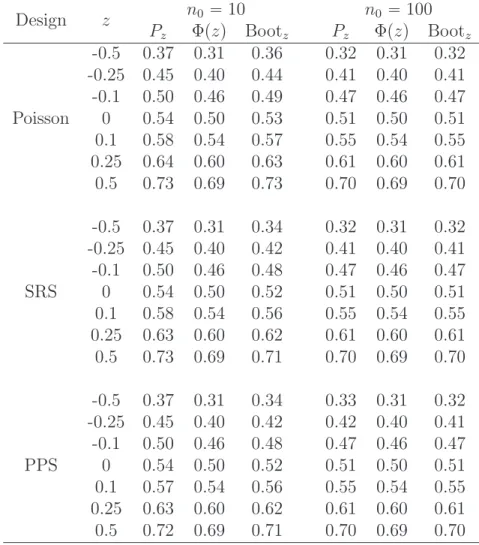
In addition, we also compare the two methods in terms of approximating the probability

P_tV˜´1{2_pY˜ _´Y¯_{q ď zu, which is obtained by 10 000 Monte Carlo simulations. We set z P}

t´0.5,_´0.25,_´0.1,0,0.1,0.25,0.5_uas done byLai and Wang(1993). Table2summarizes the simulation results. For both sample sizes, the proposed bootstrap method can approximate the target distribution well, but the performance of the Wald-type method is not as good as the proposed one when sample size is small.

Table 2: Values ofPz “PtV˜´1{2pY˜´Y¯q ďzu, the normal approximation Φpzqand the

boot-strap approximation Bootz for three sampling designs including Poisson sampling (Poisson),

SRS and PPS sampling (PPS). For convenience, we include the values Φ_pz_q for both sample sizes. Design z n0 “10 n0 “100 Pz Φpzq Bootz Pz Φpzq Bootz Poisson -0.5 0.37 0.31 0.36 0.32 0.31 0.32 -0.25 0.45 0.40 0.44 0.41 0.40 0.41 -0.1 0.50 0.46 0.49 0.47 0.46 0.47 0 0.54 0.50 0.53 0.51 0.50 0.51 0.1 0.58 0.54 0.57 0.55 0.54 0.55 0.25 0.64 0.60 0.63 0.61 0.60 0.61 0.5 0.73 0.69 0.73 0.70 0.69 0.70 SRS -0.5 0.37 0.31 0.34 0.32 0.31 0.32 -0.25 0.45 0.40 0.42 0.41 0.40 0.41 -0.1 0.50 0.46 0.48 0.47 0.46 0.47 0 0.54 0.50 0.52 0.51 0.50 0.51 0.1 0.58 0.54 0.56 0.55 0.54 0.55 0.25 0.63 0.60 0.62 0.61 0.60 0.61 0.5 0.73 0.69 0.71 0.70 0.69 0.70 PPS -0.5 0.37 0.31 0.34 0.33 0.31 0.32 -0.25 0.45 0.40 0.42 0.42 0.40 0.41 -0.1 0.50 0.46 0.48 0.47 0.46 0.47 0 0.54 0.50 0.52 0.51 0.50 0.51 0.1 0.57 0.54 0.56 0.55 0.54 0.55 0.25 0.63 0.60 0.62 0.61 0.60 0.61 0.5 0.72 0.69 0.71 0.70 0.69 0.70

6.2

Two-stage sampling designs

In this section, we test the performance of the proposed method under two-stage sampling designs. A finite population FN “ tyi,j :i“1, . . . , H;j “1, . . . , Niuis generated by

yi,j “ 50`ai`ei,j, ai „ Np0,50q, ei,j „ Expp20q,

for i _“ 1, . . . , H and j _“ 1, . . . , Ni, where Poissonpλq is a Poisson distribution with a rate

parameter λ, qi “ pai ´25q2{20, c0 “ 40 is the minimum cluster size, and H “ 100 is the

number of clusters in the finite population. The finite population size is N _“ 7 129, and the cluster sizes range from 43 to 129. We assume that the finite population size N and cluster sizes N1, . . . , NH are known. We are interested in constructing a 90% confidence

interval for the finite population mean ¯Y _“N´1řH

i“1 řNi

j“1yi,j, where the true value of ¯Y is

approximately 70.5.

We consider two different sampling designs for the first stage; one is Poisson sampling, and the other one is PPS sampling. The first-order inclusion probability (selection probability) of the i-th cluster is proportional to its cluster size Ni under Poisson (PPS) sampling for

i _“ 1, . . . , H. SRS is conducted within each selected cluster independently in the second

stage. The expected sample size of the first-stage sampling is n1, and that of the

second-stage sampling is n2. In this simulation, we consider two scenarios for the sample sizes, that

is,_pn1, n2q “ p5,10q and pn1, n2q “ p10,30q.

The derivations of the design-unbiased estimator ˜Y and its variance estimator ˜V under the two-stage sampling designs in this simulation study are presented in Appendix 9.2. We consider the following methods to construct the 90% confidence intervals for the parameters of interest.

Method I. The proposed method extended to a two-stage sampling design. This method is ap-proximately the same as that mentioned in Section 6.1 with the following two steps to bootstrap the finite population, and we set M _“1 000 for this method.

Step 1. Use the proposed method to bootstrap the H clusters by treating them as “el-ements”, and the original sample within each selected cluster are replicated ac-cordingly.

Step 2. For each bootstrap cluster, apply the proposed method to bootstrap the cluster finite population independently.

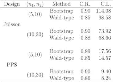
Table 3: Coverage rate and length of the 90% confidence interval for ¯Y by the proposed bootstrap method (Bootstrap) and the Wald-type method (Wald-type) under two-stage sampling designs. The first column show the first-stage sample designs, that is, Poisson sampling (Poisson) and PPS sampling (PPS), and SRS is used in the second stage. “C.R.” shows the coverage rate, and “C.L.” presents the Monte Carlo mean of the length for the 90% confidence interval. Design _pn1, n2q Method C.R. C.L. Poisson (5,10) Bootstrap 0.90 114.08 Wald-type 0.85 98.58 (10,30) Bootstrap 0.90 73.92 Wald-type 0.88 68.66 PPS (5,10) Bootstrap 0.89 17.56 Wald-type 0.85 14.57 (10,30) Bootstrap 0.90 9.40 Wald-type 0.86 8.24

Method II. Wald-type method, and it is the same as the one discussed in Section 6.1.

We conduct 1 000 Monte Carlo simulations for each scenario. Table 3 summarizes the coverage rate and average length of the constructed 90% confidence interval for the finite population mean. The coverage rates of the proposed bootstrap method are closer to 0.9 even when the sample size is limited. However, the coverage rates of the commonly used Wald-type method are not as good as the proposed bootstrap method. Specifically, the coverage rates of the Wald-type method are only around 0.86 for three scenarios, and it improves to 0.88 when sample size is large under Poisson sampling. The confidence intervals of the proposed bootstrap method are wider than those of the Wald-type method when sample size is small.

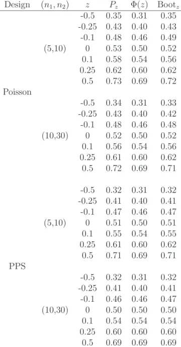
As in Section6.1, we also compare those two methods in terms of approximatingP_tV˜´1{2_pY˜_´

¯

Y_{q ď}z_u, which is obtained by 10 000 Monte Carlo simulations. We setz _{P t´}0.5,_´0.25,_´0.1,0,0.1,0.25,0.5_u. Table 4 summarizes the simulation results. For both sample sizes, the proposed bootstrap

method can approximate the target distribution well, but the performance of the Wald-type method is not as good as the proposed one especially when the sample size is small.

Table 4: Values of Pz “ PtV˜´1{2pY˜ ´Y¯q ď zu, the normal approximation Φpzq and the

bootstrap approximation Bootz under two-stage sampling designs. The first column show

the first-stage sample designs, that is, Poisson sampling (Poisson) and PPS sampling (PPS), and SRS is used in the second stage.

Design _pn1, n2q z Pz Φpzq Bootz Poisson (5,10) -0.5 0.35 0.31 0.35 -0.25 0.43 0.40 0.43 -0.1 0.48 0.46 0.49 0 0.53 0.50 0.52 0.1 0.58 0.54 0.56 0.25 0.62 0.60 0.62 0.5 0.73 0.69 0.72 (10,30) -0.5 0.34 0.31 0.33 -0.25 0.43 0.40 0.42 -0.1 0.48 0.46 0.48 0 0.52 0.50 0.52 0.1 0.56 0.54 0.56 0.25 0.61 0.60 0.62 0.5 0.72 0.69 0.71 PPS (5,10) -0.5 0.32 0.31 0.32 -0.25 0.41 0.40 0.41 -0.1 0.47 0.46 0.47 0 0.51 0.50 0.51 0.1 0.55 0.54 0.55 0.25 0.61 0.60 0.62 0.5 0.71 0.69 0.71 (10,30) -0.5 0.32 0.31 0.32 -0.25 0.41 0.40 0.41 -0.1 0.46 0.46 0.47 0 0.50 0.50 0.50 0.1 0.54 0.54 0.54 0.25 0.60 0.60 0.60 0.5 0.69 0.69 0.69

7

Conclusion

In this paper, we propose bootstrap methods for Poisson sampling, SRS and PPS sampling, and we show that the proposed bootstrap methods are second-order accurate. The first step of the proposed bootstrap methods corresponds to an inverse sampling procedure by

incorporating the sampling information. Since the proposed bootstrap method is based on an asymptotically pivotal statistic, it is necessary to estimate the variance of the design-unbiased estimator. Simulation results show that the proposed bootstrap method provides more conservative confidence interval than the Wald-type method when the sample size is small, and the 90% confidence interval constructed by the proposed bootstrap method has a better coverage rate. Although the proposed bootstrap method is discussed under the single-stage sampling designs, simulation shows that it works well under some two-single-stage sampling designs, and Edgeworth expansion for two-stage sampling designs are under investigation. It may be extended to other complex sampling designs when the asymptotic distribution of the design-unbiased estimator exists, but the second-order accuracy may not be guaranteed. Besides, the proposed bootstrap method can be easily parallelized in practice.

8

Acknowledgment

We would like to thank Dr. J. N. K. Rao for the suggestion to discuss the simple random sampling and the two anonymous reviewers for the detailed and constructive comments.

9

Supplement

9.1

Proofs

For the purpose of clarity, we explicitly expressyN,i,YN,IN,i,πN,iandpN,iforyi,Y,Ii,πi and pi to highlight that they are indexed byN, and the same notation is used for other quantities

without further mentioning. Denote E_{p¨ |} FNq and varp¨ | FNq to be the expectation and

variance with respect to the probability measure of a specific sampling design, sayP_{P oiunder}

Poisson sampling,E˚p¨qand var˚p¨qto be the conditional mean and variance with respect to the multinomial distribution in the first steps of the proposed bootstrap method conditional on the realized sample _tyN,1, . . . , yN,nu, and E˚˚p¨q and var˚˚p¨q to be the expectation and

variance with respect to the sampling design in the second step conditional on the bootstrap finite population F˚

N.

Proof of Lemma 3.1. DenoteX_N,ip1q _“n0N´2yN,i2 p1´πN,iqπ´N,i2pIN,i´πN,iq, thenn0N´2 `ˆ VN,P oi´ VN,P oi ˘ “řN i“1X p1q N,i. Let D p1q N be the event řN i“1X p1q N,i ąǫ ( for N <sub>P</sub> N<sub>`, whereǫ P p0,8q</sub>

and N_{` is the set of positive integers.}

By the Borel-Cantelli Lemma (Athreya and Lahiri;2006, Thereom 7.2.2), to show (1), it is enough to prove 8 ÿ N“1 P_{P oipD}p1q N q ă 8 (A.1)

forǫ_ą0. By the Markov’s inequality (Athreya and Lahiri;2006, Proposition 6.2.4), we have

P_{P oipD}p_N1q_{q ď ǫ}´4_E $ & % ˜_N ÿ i“1 X_N,ip1q ¸4 |FN , . -“ ǫ´4 „ N ÿ i“1 E " ´ X_N,ip1q¯4 _|FN * ` ÿ pi,jqPΓN E " ´ X_N.ip1q¯ 2 |FN * E " ´ X_N,jp1q¯ 2 |FN *  ,

where the last equality holds since E_pX_N,ip1q _|FNq “0 for i“1, . . . , N, and X

p1q

N,i is

indepen-dent of X_N,jp1q for_pi, j_{q P} ΓN with ΓN “ tpi, jq:i, j “1, . . . , N and i‰ju.

Consider E " ´ X_N,ip1q¯4 _|FN * “ n40N´ 8

yN,i8 p1´πN,iq5π´_N,i4tp1´πN,iq3π_N,i´3 `1u ď C1,1n´03N

´1_y8

N,i, (A.2)

Next, consider E " ´ X_N,ip1q¯ 2 |FN *

“ n20N´4yN,i4 πN,i´3p1´πN,iq3 ď C1,2n´01N

´1_y4

N,i, (A.3)

where C1,2 is a positive constant.

Based on some algebra and (C3), we have

ÿ

pi,jqPΓN

y_N,i4 y_N,j4 _“ O_pN2_q. (A.4) By (A.2), (A.3) and (A.4), we have

P_{P oipD}p1q N q ď ǫ´4C1,1n´03N´ 1 N ÿ i“1 y_N,i8 _`ǫ´4C₁2_,2n´₀2N´2 ÿ pi,jqPΓN y_N,i4 y_N,j4 “ O_pN´2α_q

for any fixed ǫ _ą0, where the last inequality holds by (C3). Since α _{P p}2´1_,1

s by (C1), we have proved (1) based on (A.1).

For µp_{N,P oi}3q _“řN

i“1y 3

N,ip1´πN,iqtp1´πN,iq2πN,i´2 ´1u, we have

ˇ ˇ ˇn 2 0N ´3_µp3q P oi ˇ ˇ ˇ “ n2₀N´3 N ÿ i“1

y_N,i3 _p1_´πN,iqtp1´πN,iq2π´N,i2 ´1u

ď 2n2₀N´3 N ÿ i“1 |yN,i|3πN,i´2 ď 2C₁´2N´1 N ÿ “1 |yN,i|3 “Op1q,

where the first inequality holds by 0_ăπN,iă1 and 0ă1´πN,iă1, the second inequality

Mentioned that E´n20N´3µˆ p3q N,P oi|FN ¯ “ E « n20N´3 n ÿ i“1

yN,i3 p1´πN,iqπN,i´1tp1´πN,iq2πN,i´2 ´1u |FN

ff

“ n20N´3

N

ÿ

i“1

yN,i3 p1´πN,iqtp1´πN,iq2π´N,i2 ´1u “ n2₀N´3µp_{N,P oi}3q and var´µˆp_{N,P oi}3q _|FN ¯ “ var « n20N´ 3 n ÿ i“1

yN,i3 p1´πN,iqπN,i´1tp1´πN,iq2π´N,i2 ´1u |FN

ff ď 4n4₀N´6 N ÿ i“1 y_N,i6 π_N,i´5 “ O_pn´₀1_q,

we can obtain that n20N´3pµˆ

p3q

N,P oi´µ

p3q

N,P oiq “ Oppn

´1{2

0 q by the Markov’s inequality. The

results concerning τ_{N,P oi}p3q and ˆτ_{N,P oi}p3q can be proved similarly and is omitted here. Thus, we finalize the proof of Lemma 3.1.

The following lemmas are useful in establishing Theorem 3.1 and 3.2.

Lemma 9.1. Denote XN,i “ V

´1{2

N,P oiyN,iπN,i´1pIN,i ´ πN,iq for i “ 1, . . . , N. Let ∆N,1 “ řN

i“1XN,i and φ∆N,1ptq “Etexppιt∆N,1q |FNu be the characteristic function (c.f.) of ∆N,1, where ι is the imaginary unit. Then under conditions (C1)–(C3),

ˇ ˇφ_∆N,1ptq ˇ ˇ ď expp´t2{3q, (A.5) ˇ ˇφ∆N,1ptq ´expp´t 2 {2_qˇ ˇ ď 16|t|3V ´3{2 N,P oiν p3q N,P oiexpp´t 2 {3_q (A.6)

for all _|t_{| ď} V_{N,P oi}3{2 _{´4ν_{N,P oi}p3q ¯, where ν_{N,P oi}p3q _“ řN

i“1|yN,i|3p1 ´πN,iq p1´πN,iq2πN,i´2 `1

( . Furthermore, ˇ ˇ ˇφ∆N,1ptq ´expp´t 2 {2q ´6´1pιt_q3V_{N,P oi}´3{2µp_{N,P oi}3q expp´t2_{2qˇˇ ˇ ď C2,1expp´19t2{48q ` t4n´01`t 6 n´01 ˘ (A.7)

for all _|t_{| ď}min´ max1ďiďNEpXN,i2 |FNq

(´1{2

, V_{N,P oi}3{2 _{´4ν_{N,P oi}p3q ¯¯, where C2,1 is a positive

constant and recall that µp_{N,P oi}3q _“řN

i“1yN,i3 p1´πN,iqtp1´πN,iq2π´N,i2 ´1u.

Proof. As IN,i „BerpπN,iq, EpXN,i | FNq “ 0 and EpXN,i2 | FNq “VN,P oi´1 yN,i2 p1´πN,iqπ´N,i1

for i_“1, . . . , N. In addition,

E_pX_N,i3 _|FNq “ V´

3{2

N,P oiy

3

N,ip1´πN,iq p1´πN,iq2πN,i´2 ´1

(

and

E_t|XN,i|3 |FNu “V´

3{2

N,P oi|yN,i|3p1´πN,iq p1´πN,iq2πN,i´2 `1

( . Thus, řN i“1EpXN,i2 | FNq “ 1, řN i“1EpXN,i3 | FNq “ V ´3{2 N,P oiµ p3q N,P oi “ Opn ´1{2 0 q by (C2) and Lemma 3.1. In addition, ν_{N,P oi}p3q _“řN

i“1|yN,i|3p1´πN,iq p1´πN,iq2πN,i´2 `1

( “O_pn´02N´3q, which impliesřN i“1Et|XN,i|3 |FNu “ V ´3{2 N,P oiν p3q N,P oi“Opn ´1{2

0 q.By the fact that max1ďiďNEt|XN,i|3 |

FNu ď řN_i“1Et|XN,i|3 | FNu “Opn´

1{2

0 q,Et|XN,i|3 |FNu ă 8 for i“1, . . . , N. By Lemma

5.1 of Petrov (1995), ˇ ˇφ_∆N,1ptq ˇ ˇ ď expp´t2{3q, ˇ ˇφ∆N,1ptq ´expp´t 2 {2qˇ ˇ ď 16|t|3V ´3{2 N,P oiν p3q N,P oiexpp´t 2 {3q for all _|t_{| ď}V_{N,P oi}3{2 _{´4ν_{N,P oi}p3q ¯.

function of XN,i. Note that for any complex numbers z, w, |exppzq ´1´w| ď p|z´w| ` |w_|2_{{2qexptmaxp|z|,|w|qu, it follows that}

ˇ ˇ ˇφ∆N,1ptq ´expp´t 2 {2_{q ´}6´1_pιt_q3V_{N,P oi}´3{2µp_{N,P oi}3q exp_p´t2_{2_qˇˇ ˇ “ ˇ ˇ ˇ ˇ ˇ N ź i“1 φXN,iptq ´expp´t2{2q ´6´1pιtq3V ´3{2 N,P oiµ p3q N,P oiexpp´t 2 {2_q ˇ ˇ ˇ ˇ ˇ “ exp_p´t2_{2_q ˇ ˇ ˇ ˇ ˇ exp «_N ÿ i“1 log_tφXN,iptqu `t 2 {2 ff ´1<sub>´</sub>6´1<sub>p</sub>ιt<sub>q</sub>3V<sub>N,P oi</sub>´3{2µp<sub>N,P oi</sub>3q ˇ ˇ ˇ ˇ ˇ ď exp<sub>p´</sub>t2<sub>{</sub>2<sub>q</sub> „ˇ ˇ ˇ ˇ N ÿ i“1 log<sub>t</sub>φXN,iptqu `t 2 {2_´6´1_pιt_q3V_{N,P oi}´3{2µp_{N,P oi}3q ˇ ˇ ˇ ˇ `2´1ˇˇ ˇ6 ´1 pιt<sub>q</sub>3V<sub>N,P oi</sub>´3{2µp<sub>N,P oi</sub>3q ˇˇ ˇ 2 ˆexp # max ˜ˇ ˇ ˇ ˇ ˇ N ÿ i“1 log<sub>t</sub>φXN,iptqu `t2{2 ˇ ˇ ˇ ˇ ˇ , ˇ ˇ ˇ6 ´1 pιt_q3V_{N,P oi}´3{2µp_{N,P oi}3q ˇ ˇ ˇ ¸+ .

By Lemma 11.4.3 of Athreya and Lahiri(2006),

ˇ ˇ ˇ ˇ ˇ N ÿ i“1 log_tφXN,iptqu `t2{2´6´1pιtq3V ´3{2 N,P oiµ p3q N,P oi ˇ ˇ ˇ ˇ ˇ (A.8) ď N ÿ i“1 ˇ

ˇlogtφ_XN,iptqu ´2´1pιtq2EpX_N,i2 |F_Nq ´6´1pιtq3EpX_N,i3 |F_Nq ˇ ˇ ď N ÿ i“1 `

E“min _|tXN,i|3{3,ptXN,iq4{24

( |FN ‰ `t4_tE_pXN,i2 |FNqu2{4 ˘ ď C2,2t4n´01

for all _|t_{| ď} max1ďiďNEpXN,i2 | FNq

(´1{2

, where C2,2 is a positive constant and the last

inequality is by the fact that

N ÿ i“1 E_pX_N,i4 _|FNq “ V_{N,P oi}´2 N ÿ i“1

yN,i4 p1´πN,iqtp1´πN,iq3π´N,i3 `1u “ O_pn´₀1_q.

Similarly, by Lemma 11.4.3 of Athreya and Lahiri(2006), ˇ ˇ ˇ ˇ ˇ N ÿ i“1 log_tφXN,iptqu `t 2 {2 ˇ ˇ ˇ ˇ ˇ ď N ÿ i“1 ˇ

ˇlogtφXN,iptqu ´2´1pιtq2EpXN,i2 |FNq

ˇ ˇ ď 5_|t_|3 N ÿ i“1 E_t|XN,i|3 |FNu{12“5|t|3V´ 3{2 N,P oiν p3q N,P oi{12

for all _|t_{| ď} max1ďiďN EpXN,i2 |FNq

(´1{2

. Thus, if _|t_{| ď}min´ max1ďiďNEpXN,i2 |FNq

(´1{2 , V_{N,P oi}3{2 _{´4ν_{N,P oi}p3q ¯¯, max ˜ˇ ˇ ˇ ˇ ˇ N ÿ i“1 log_tφXN,iptqu `t2{2 ˇ ˇ ˇ ˇ ˇ , ˇ ˇ ˇ6 ´1 pιt_q3V_{N,P oi}´3{2µp_{N,P oi}3q ˇ ˇ ˇ ¸ (A.9) ď 5t2_{48. Mentioned that 2´1ˇˇ ˇ6 ´1 pιt_q3V_{N,P oi}´3{2µp_{N,P oi}3q ˇˇ ˇ 2 ďC2,3t6n´01 (A.10)

for some positive constant C2,3.

Finally, by (A.8), (A.9) and (A.10), it follows that

ˇ ˇ ˇφ∆N,1ptq ´expp´t 2 {2_{q ´}6´1_pιt_q3V_{N,P oi}´3{2µp_{N,P oi}3q exp_p´t2_{2_qˇˇ ˇ ď exp_p´t2_{2_q` C2,2t4n´01`C2,3t6n´01 ˘ exp_p5t2_{48_q ď C2,1expp´19t2{48q ` t4n´<sub>0</sub>1<sub>`</sub>t6n´₀1˘

for all _|t_{| ď} min´ max1ďiďNEpXN,i2 |FNq

(´1{2

, V_{N,P oi}3{2 _{´4ν_{N,P oi}p3q ¯¯. This concludes the proof of this Lemma.

Lemma 9.2. Denote ∆N,2 “ ´2´1V ´3{2 N,P oi ÿ pi,jqPΓN yN,iy2N,jp1´πN,jqπN,i´1π ´2 N,jpIN,i´πN,iqpIN,j ´πN,jq,

then under conditions (C1)–(C3),

E_t∆N,2exppιt∆N,1q |FNu “ 2´1_t2_exp

p´t2_{2_qV_{N,P oi}´5{2Θ_{N,P oi}p2,3q _`̟N,1ptq,

for all _|t_{| ď} max1ďiďN EpXN,i2 |FNq

(´1{2

, where XN,i“V_{N,P oi}´1{2yN,iπ_N,i´1pIN,i´πN,iq, ∆N,1 “ řN

i“1XN,i, ΓN “ tpi, jq:i, j “1, . . . , N and i‰ju,

Θp_{N,P oi}2,3q _“ ÿ

pi,jqPΓN

y_N,i2 y_N,j3 _p1_´πN,iqp1´πN,jq2π´N,i1π

´2 N,j, and ̟N,1ptq satisfies |̟N,1ptq| ď C3,1exp " ´t2_{2_{`</sub>2<sub>|</sub>t<sub>|</sub>3V<sub>N,P oi</sub>´3{2ν<sub>N,P oi</sub>p3q <sub>{</sub>3<sub>`}t2 max 1ďiďNEpX 2 N,i|FNq * ˆ´|t_|3n´01`t4n ´3{2 0 ` |t|5n´01 ¯ ,

with C3,1 being a positive constant and νp 3q

N,P oi“

řN

i“1|yN,i| 3

p1_´πN,iq p1´πN,iq2π´N,i2 `1

( . Proof. First, write

E_tpIN,i´πN,iqexppιtXN,iq |FNu “ ιtV

´1{2

for i_“1, . . . , N, where

|̟N1,iptq|

“ |E_tpIN,i´πN,iqexppιtXN,iq |FNu ´ιtV´

1{2 N,P oiyN,ip1´πN,iq| “ p1_´πN,iqπN,i ˇ ˇ ˇ ˇ „

exp!ιtV_{N,P oi}´1{2yN,ip1´πN,iqπN,i´1

)

´1

´ιtV_{N,P oi}´1{2yN,ip1´πN,iqπ´N,i1

 ´!exp´_´ιtV_{N,P oi}´1{2yN,i ¯ ´1<sub>`</sub>ιtV<sub>N,P oi</sub>´1{2yN,i )ˇ ˇ ˇ ˇ ď 2´1<sub>p</sub>1<sub>´</sub>πN,iqπN,i " ˇ ˇ ˇtV ´1{2 N,P oiyN,ip1´πN,iqπ ´1 N,i ˇ ˇ ˇ 2 `ˇˇ ˇtV ´1{2 N,P oiyN,i ˇ ˇ ˇ 2* ď C3,2t2N´1yN,i2 ,

and C3,2 is a positive constant. The last but one inequality is due to the fact that for any

real number x, _|exp_pιx_{q ´}1_´ιx_{| ď |}x_|2_{{2. As a consequence, for any pi, jq PΓ}

N, E_tpIN,i´πN,iqexppιtXN,iq |FNuEtpIN,j ´πN,jqexppιtXN,jq |FNu “ !ιtV_{N,P oi}´1{2yN,ip1´πN,iq `̟N1,iptq

) !

ιtV_{N,P oi}´1{2yN,jp1´πN,jq `̟N1,jptq

)

“ ´t2V_{N,P oi}´1 yN,iyN,jp1´πN,iqp1´πN,jq `̟N2,ijptq,

where |̟N2,ijptq| ď ˇˇ ˇtV ´1{2 N,P oiyN,ip1´πN,iq̟N1,jptq ˇ ˇ ˇ` ˇ ˇ ˇtV ´1{2 N,P oiyN,jp1´πN,jq̟N1,iptq ˇ ˇ ˇ ` |̟N1,iptq̟N1,jptq| ď C3,3 ! |t_|3n1₀{2N´2_py_N,i2 _|yN,j| ` |yN,i|yN,j2 q `t 4_N´2_y2 N,iy 2 N,j )

with C3,3 being a positive constant.

the proof of Lemma 5.1 of Petrov (1995), we can show that ˇ ˇ ˇ ˇ ˇ ź k‰i,j φXN,kptq ˇ ˇ ˇ ˇ ˇ ď exp # ´t2 ÿ k‰i,j E_pX_N,k2 _|FNq{2`2|t|3 ÿ k‰i,j E_t|XN,k|3 |FNu{3 + .

Using the inequality _|exp_pz_{q ´}1_{| ď |}z_|exp_p|z_|q for all complex number z, we can obtain that ˇ ˇ ˇ ˇ ˇ ź k‰i,j φXN,kptq ´expp´t 2 {2_q ˇ ˇ ˇ ˇ ˇ “ exp_p´t2_{2_q ˇ ˇ ˇ ˇ ˇ exp « ÿ k‰i,j log_tφXN,kptqu `t 2 {2 ff ´1 ˇ ˇ ˇ ˇ ˇ ď exp<sub>p´</sub>t2<sub>{</sub>2<sub>q</sub> ˇ ˇ ˇ ˇ ˇ ÿ k‰i,j log<sub>t</sub>φXN,kptqu `t2{2 ˇ ˇ ˇ ˇ ˇ exp «ˇ ˇ ˇ ˇ ˇ ÿ k‰i,j log_tφXN,kptqu `t2{2 ˇ ˇ ˇ ˇ ˇ ff

By Lemma 11.4.3 of Athreya and Lahiri(2006),

ˇ ˇ ˇ ˇ ˇ ÿ k‰i,j log_tφXN,kptqu `t2{2 ˇ ˇ ˇ ˇ ˇ ď ÿ k‰i,j ˇ ˇlogtφXN,kptqu ´2 ´1 pιt<sub>q</sub>2E<sub>p</sub>X<sub>N,k</sub>2 <sub>|</sub>FNq ˇ ˇ `2´1t2E_pXN,i2 |FNq `2´1t2EpXN,j2 |FNq ď 5<sub>|</sub>t<sub>|</sub>3 ÿ k‰i,j E<sub>t|</sub>XN,k|3 |FNu{12`2´1t2 EpXN,i2 |FNq `EpXN,j2 |FNq ( .

for all _|t_{| ď} max1ďiďNEpXN,i2 |FNq (´1{2 . Thus, we obtain ˇ ˇ ˇ ˇ ˇ ź k‰i,j φXN,kptq ´expp´t 2 {2_q ˇ ˇ ˇ ˇ ˇ ď exp # ´t2 ÿ k‰i,j E_pX_N,k2 _|FNq{2`5|t|3 ÿ k‰i,j E<sub>t|</sub>XN,k|3 |FNu{12 + ˆ „ 5|t<sub>|</sub>3 ÿ k‰i,j E<sub>t|</sub>XN,k|3 |FNu{12 `2´1t2 E_pXN,i2 |FNq `EpXN,j2 |FNq ( 

for all |t_{| ď} max1ďiďNEpXN,i2 |FNq

(´1{2 . Finally, we have E_t∆N,2exppιt∆N,1q |FNu “ ´2´1_V´3{2 N,P oi ÿ pi,jqPΓN yN,iy2N,jp1´πN,jqπN,i´1π ´2 N,j

ˆE_tpIN,i´πN,iqpIN,j ´πN,jqexppιt∆N,1q |FNu “ ´2´1V_{N,P oi}´3{2 ÿ pi,jqPΓN yN,iy2N,jp1´πN,jqπN,i´1π ´2 N,j ź k‰i,j φXN,kptq ˆE_tpIN,i´πN,iqexppιtXN,iq |FNu ˆE_tpIN,j´πN,jqexppιtXN,jq |FNu “ ´2´1V_{N,P oi}´3{2 ÿ pi,jqPΓN yN,iy2N,jp1´πN,jqπ_N,i´1π_N,j´2 ź k‰i,j φXN,kptq

ˆ ´t2V_{N,P oi}´1 yN,iyN,jp1´πN,iqp1´πN,jq `̟N2,ijptq

(

“ 2´1_t2_V´5{2

N,P oi

ÿ

pi,jqPΓN

yN,i2 y3N,jp1´πN,iqp1´πN,jq2πN,i´1π

´2 N,j ź k‰i,j φXN,kptq ´2´1V_{N,P oi}´3{2 ÿ i‰j yN,iyN,j2 p1´πN,jqπN,i´1π ´2 N,j ź k‰i,j φXN,kptq̟N2,ijptq “ 2´1_t2_exp p´t2_{2_qV_{N,P oi}´5{2Θ_{N,P oi}p2,3q _`̟N,1ptq

for all _|t_{| ď} max1ďiďNEpXN,i2 |FNq (´1{2 and ̟N,1ptqsatisfies |̟N,1ptq| ď C3,4exp # ´t2_{2<sub>`</sub>2<sub>|</sub>t<sub>|</sub>3 N ÿ i“1 E<sub>t|</sub>XN,i|3 |FNu{3`t2 max 1ďiďNEpX 2 N,i|FNq + ˆ " |t_|3n´₀1N´2ÿ i‰j ` |yN,i|3|yN,j|3`yN,i2 y 4 N,j ˘ `t4n´<sub>0</sub>3{2N´2ÿ i‰j |yN,i|3yN,j4 `t4n´₀1{2N´3ÿ i‰j py4_N,i|yN,j|3`yN,i2 |yN,j|5q ` |t_|5n´01 ˆ N´2ÿ i‰j yN,i2 |yN,j|3 ˙ˆ N´1 N ÿ i“1 |yN,i|3 ˙* ď C3,1exp " ´t2_{2_{`</sub>2<sub>|</sub>t<sub>|</sub>3V<sub>N,P oi</sub>´3{2ν<sub>N,P oi</sub>p3q <sub>{</sub>3<sub>`}t2 max 1ďiďNEpX 2 N,i|FNq * ˆ´|t_|3n´₀1_{`</sub>t4n<sub>0</sub>´3{2<sub>` |}t_|5n´₀1¯,

where C3,4 is a positive constant.

Lemma 9.3. Denote YˆN,P oi “

řN

i“1yN,iπN,i´1IN,i, YN “

řN i“1yN,i and VˆN,P oi “ řN i“1y 2 N,ip1´ πN,iqπ_N,i´2IN,i, then under conditions (C1)–(C3),

ˆ V_{N,P oi}´1{2 ´YˆN,P oi´YN ¯ “∆N,1`∆N,2`∆N,3`∆N,4, where ∆N,1 “ V´ 1{2 N,P oi N ÿ i“1

yN,iπN,i´1pIN,i´πN,iq,

∆N,2 “ ´2´1V´ 3{2 N,P oi ÿ pi,jqPΓN yN,iyN,j2 p1´πN,jqπ´N,i1π ´2 N,jpIN,i´πN,iqpIN,j´πN,jq, ∆N,3 “ ´2´1V´ 3{2 N,P oi N ÿ i“1

and recall that ΓN “ tpi, jq:i, j “1, . . . , N and i‰ju. In addition, ∆N,4 satisfies P_{P oi}´_{|∆N,4| ěn}´₀1{2_plogn0q´1¯_“opn´₀1{2_q. Proof. Denote ΛN,1 “ VN,P oi´1 řN i“1y 2

N,ip1´πN,iqπN,i´2pIN,i´πN,iq. Mentioned that EpΛN,1 |

FNq “0 and E`Λ2N,1 |FN ˘ “V_{N,P oi}´2 N ÿ i“1

y_N,i4 _p1´πN,iq3πN,i´3 “Opn´

1 0 q, we have that ΛN,1 “Oppn´ 1{2 0 q. In addition, E_pΛ4 N,1 |FNq “ E « " V_{N,P oi}´1 N ÿ i“1

y_N,i2 _p1_´πN,iqπN,i´2pIN,i´πN,iq

*4 |FN ff “ V_{N,P oi}´4 „ N ÿ i“1

yN,i8 p1´πN,iq5πN,i´4 p1´πN,iq3π´N,i3 `1

(

` ÿ

pi,jqPΓN

y_N,i4 y_N,j4 _p1_´πN,iq3p1´πN,jq3π_N,i´3π_N,j´3

 “ O_pn´₀2_q. By some algebra, ˆ V_{N,P oi}´1{2 ´YˆN,P oi´YN ¯ “ # V_{N,P oi}´1{2 N ÿ i“1

yN,iπ_N,i´1pIN,i´πN,iq

+ p1_`ΛN,1q´1{2 “ # V_{N,P oi}´1{2 N ÿ i“1

yN,iπN,i´1pIN,i´πN,iq

+

Use the notations of ∆N,1, ∆N,2 and ∆N,3, we have ˆ V_{N,P oi}´1{2 ´YˆN,P oi´YN ¯ “ ∆N,1 1´2´1ΛN,1`OppΛ2N,1q ( “ ∆N,1´2´1∆N,1ΛN,1`Opp∆N,1Λ2N,1q “ ∆N,1`∆N,2 `∆N,3`ΛN,2`Opp∆N,1Λ2N,1q where ΛN,2 “ ´2´1V ´3{2 N,P oi N ÿ i“1

y3N,ip1´πN,iqπ´N,i3 pIN,i´πN,iq2´EpIN,i´πN,iq2

( . It remains to show P_{P oi}´_{|ΛN,2| ěn}´1{2 0 plogn0q´1 ¯ “o_pn´₀1{2_q (A.11) and P_{P oi}´_|∆N,1Λ2 N,1| ěn ´1{2 0 plogn0q´1 ¯ “o_pn´₀1{2_q. (A.12) For (A.11), it is a directly consequence of

E_pΛN,2 |FNq “0 and E` Λ2N,2 |FN ˘ “O_pn´₀2_q.