The reparameterization trick for acquisition functions

The reparameterization trick for acquisition functions

Marc Peter Deisenroth1 [email protected] 1_{Imperial College of London} 2_{University of Freiburg}

Abstract

Bayesian optimization is a sample-efficient approach to solving global optimiza-tion problems. Along with a surrogate model, this approach relies on theoreti-cally motivated value heuristics (acquisition functions) to guide the search process. Maximizing acquisition functions yields the best performance; unfortunately, this ideal is difficult to achieve since optimizing acquisition functionsper seis fre-quently non-trivial. This statement is especially true in the parallel setting, where acquisition functions are routinely non-convex, high-dimensional, and intractable. Here, we demonstrate how many popular acquisition functions can be formulated as Gaussian integrals amenable to the reparameterization trick [14, 17] and, ensu-ingly, gradient-based optimization. Further, we use this reparameterized represen-tation to derive an efficient Monte Carlo estimator for the upper confidence bound acquisition function [19] in the context of parallel selection.

1

Introduction

In Bayesian optimization (BO), acquisition functions𝐻, with few exceptions, amount to integrals defined in terms of a belief𝑝over the unknown outcomes𝐲= {𝑦₁,…, 𝑦_𝑞}revealed when evaluating a black-box function𝑓 at corresponding input locations𝐗 = {𝐱₁,…,𝐱_𝑞}. This formulation natu-rally occurs as part of a Bayesian approach whereby we would like to assess how valuable different queries𝐗are to the optimization process by accounting for all conceivable realizations of𝐲=𝑓(𝐗). Denoting byℎthe function used to convey the value-added for observing a given realization, this paradigm gives rise to acquisition functions defined as

𝐻(𝐗;𝝓) =

∫_ℎ(𝐲;𝝓)𝑝(𝐲|𝐗,)𝑑𝐲, (1)

where integration region ⊆  represents the set of all possible outcomes𝐲,𝝓 any additional parameters associated with integrandℎ, andthe available prior information.1Without loss of gen-erality, we express acquisition functions as𝑞-dimensional integrals, where𝑞denotes the total number of queries with unknown outcomes after each decision. For pool-size𝑞= 1, we recover strictly se-quential decision-making rules; whereas, for𝑞 >1, we obtain strategies for parallel selection.2 _As an exception to this rule,non-myopicacquisition functions, which assign value by further consider-ing how different realizations of(𝐗,𝐲)impact our broader understanding of black-box𝑓, generally correspond to higher-dimensional integrals. Specifically, non-myopic instances of the above formu-lation typically recurse, with the integrandℎamounting to an additional integral of the form (1). While in a minority of cases closed-form solutions exist, these integrals are generally intractable and therefore difficult to optimize.

1_{Henceforth, we omit explicit reference to prior information.}

2_{To avoid confusion when discussing SGD, we reserve the termbatch-sizefor description of minibatches.}

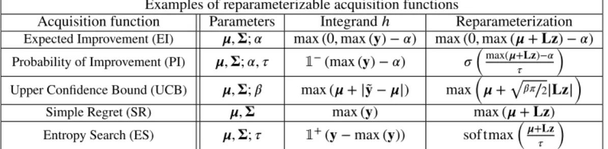
Examples of reparameterizable acquisition functions

Acquisition function Parameters Integrandℎ Reparameterization

Expected Improvement (EI) 𝝁,𝚺;𝛼 max (0,max (𝐲) −𝛼) max (0,max (𝝁+𝐋𝐳) −𝛼)

Probability of Improvement (PI) 𝝁,𝚺;𝛼, 𝜏 1−(max (𝐲) −𝛼) 𝜎

(

max(𝝁+𝐋𝐳)−𝛼 𝜏

)

Upper Confidence Bound (UCB) 𝝁,𝚺;𝛽 max (𝝁+|𝐲̃−𝝁|) max(𝝁+√𝛽𝜋_∕2|_𝐋𝐳|

)

Simple Regret (SR) 𝝁,𝚺 max (𝐲) max (𝝁+𝐋𝐳)

Entropy Search (ES) 𝝁,𝚺;𝜏 1+(𝐲− max (𝐲)) sof tmax

(

𝝁+𝐋𝐳

𝜏

)

Table 1: Above, we use the following notation: Cholesky factor𝐋𝐋⊤≜𝚺;1+∕−denotes the right-/left-continuous Heaviside step function;𝜎the sigmoid nonlinearity;𝛼the improvement threshold; 𝜏 the temperature parameter described in Section 2; and, random variables𝐲̃ ∼ (𝝁,𝛽𝜋_∕2𝚺). For Entropy Search, a non-myopic acquisition function, only the innermost integrand (used to approximate𝑝_𝑚𝑎𝑥) and its corresponding reparameterization are shown.

For this reason, a variety of methods have been proposed for evaluating intractable acquisition func-tions. These approaches have ranged from expectation propagation-based approximations of Gaus-sian probabilities [5, 9, 10] to bespoke approximation strategies [4, 6] to sample-based Monte Carlo techniques [9, 16, 18].

The special case of parallel Expected Improvement (𝑞-EI) has received considerable attention [3, 7, 18, 20]; however, excepting [20], proposed methods do not scale gracefully in pool-size𝑞. Still within the context of𝑞-EIand independent of our work, [20] derive results analogous to our own, but refer to the reparameterization trick (discussed below) asinfinitesimal perturbation analysis[8]. In this work, we focus on the most common estimation technique: Monte Carlo integration. De-spite their generality and myriad other desirable properties, Monte Carlo approaches have consis-tently been regarded as non-differentiable and, therefore, inefficient in practice given the need to optimize (1). However, it seems to have been overlooked that sample-based approaches can indeed be used to estimate gradients, well-known examples of which include stochastic backpropagation and the reparameterization trick [14, 17]. In the following, we exploit this insight to demonstrate gradient-based optimization of acquisition functions estimated via Monte Carlo integration. Thereparameterization trickis a way of rewriting functions of random variables that makes their differentiability w.r.t. the parameters of an underlying distribution transparent. The trick applies a deterministic mapping𝜌 ∶  →  from random variables𝐳 ∈ with a parameter-free base distribution to random variables𝐲 ∈with the target distribution. This change of variables helps clarify that ifℎis a differentiable function of 𝐲 = 𝜌(𝐳;𝜽)then, by the chain rule of derivatives

𝑑ℎ 𝑑𝜽 =

𝑑ℎ 𝑑𝜌

𝑑𝜌

𝑑𝜽, i.e., we can use gradient information to optimize the target distribution’s parameters𝜽.

We now explore the importance of this fact for BO and, in particular, for parallel selection.

2

Reparameterizing acquisition functions

As is arguably the natural way of expressing uncertainty over interrelated values, beliefs𝑝(𝐲|𝐗)

over the𝑞outcomes for pool𝐗are typically defined in terms of a multivariate normal distribution

(𝝁,𝚺). In the context of the reparameterization trick, the corresponding deterministic mapping for Gaussian random variables𝐲is𝜌(𝐳;𝝁,𝚺)≜𝝁+𝐋𝐳, where𝐋denotes the Cholesky factor of𝚺, s.t.𝐋𝐋⊤=𝚺and𝐳∼(𝟎,𝐈). Rewriting (1) as a Gaussian integral and reparameterizing, we have

𝐻(𝐗;𝝓) = ∫ 𝐛 𝐚 ℎ(𝐲;𝝓)(𝐲;𝝁,𝚺)𝑑𝐲= ∫ 𝐛′ 𝐚′ ℎ(𝝁+𝐋𝐳;𝝓′)(𝐳;𝟎,𝐈)𝑑𝐳, (2)

where each of the𝑞terms𝑐_𝑖′in both𝐚′_and𝐛′_{is transformed as𝑐}′

𝑖 = (𝑐𝑖 −𝜇𝑖−

∑

𝑗<𝑖𝐿𝑖𝑗𝑧𝑗)∕𝐿𝑖𝑖 and where values in𝝓′have similarly been mapped to. By taking the gradient of𝐻(𝐗;𝝓)w.r.t. model-based posterior_(𝝁,𝚺) =(𝐗)and further differentiating through the model to inputs𝐗, we can perform gradient ascent on acquisition values.3

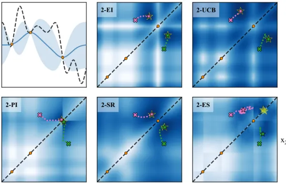
2-EI 2-UCB

2-PI 2-SR 2-ES

x

x

Figure 1: Top left: GP-based posterior over 1-dimensional black-box𝑓 given three initial obser-vations (orange dots). Remaining: Response surfaces of various acquisition functions for pool-size 𝑞= 2. From ‘×’ to ‘☆’, paths explored by gradient descent (green) and stochastic gradient descent (pink) when optimizing the various acquisition functions. Dashed horizontal lines denote axes of symmetry and large ‘☆’ (yellow) indicate the global maximum of each acquisition function. When Monte Carlo integrating (2), an unbiased estimate to the acquisition gradients is then

𝑑𝐻(𝐗;𝝓) 𝑑𝐗 ≈ 1 𝑛 ∑𝑛 𝑘=1 𝑑ℎ(𝐲_𝑘;𝝓) 𝑑𝐲_𝑘 𝑑𝐲_𝑘 𝑑(𝐗) 𝑑(𝐗) 𝑑𝐗 , (3)

where, by minor abuse of notation, we have substituted in𝐲_𝑘 = 𝜌(𝐳_𝑘;(𝐗)). The availability of gradient information is especially important for𝑞 > 1, both because parallel acquisition functions are generally intractable and because the dimensionality of the acquisition space scales linearly in𝑞. Examples of well-known acquisition functions amenable to this treatment are presented in Table 1. Figure 1 provides a visual example of the corresponding (stochastic) gradient ascent process, for each of the five acquisition functions shown in the table. Before going further, several points of interest in Table 1 warrant attention:

1. Parallelizing UCB: To the best of our knowledge, the integral representation ofUCBis novel and leads to the first truly parallel formulation ofUCB(𝑞-UCB). Relevantly, using the reparam-eterization trick greatly simplifies the associated derivation. As with other acquisition functions discussed here,𝑞-UCBcan be efficiently estimated via Monte Carlo and optimized using gradi-ents. For the complete derivation and related formulae, please refer to Appendix A.

2. Relaxing Heaviside step functions: Both Probability of Improvement (PI) and Entropy Search (ES) contain Heaviside step functions, whose derivatives are Dirac delta functions. Since these gradients are zero a.e., we instead propose the use of asof tmaxfunction with temperature param-eter𝜏. This combination has the appealing property that the resulting approximation becomes exact as𝜏→0, a property recently exploited in [11, 15]. To the extent that this soft approxima-tion introduces an addiapproxima-tional source of error, we argue that this downside is largely outweighed by the availability of informative gradients, which enable us to greatly reduce optimization error [2]. 3. Differentiating though the max(): Many acquisition functions, such asEI, use the max operator. While not technically differentiable, this operator is known to be subdifferentiable and affords well-behaved (sub)gradients.

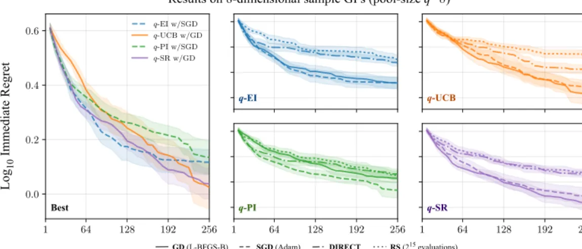
1 64 128 192 256 0.0 0.2 0.4 0.6 qq-EI w/SGD-UCB w/GD q-PI w/SGD q-SR w/GD 1 64 128 192 256 1 64 128 192 256 Best q-EI q-UCB q-PI q-SR L og10 Im m edi at e Re gre t

Results on 8-dimensional sample GPs (pool-size q=8)

GD (L-BFGS-B) SGD (Adam) DIRECT RS (215 _evaluations)

Figure 2: Left: For equivalent runtimes, best average case performance of each acquisition function given 256 evaluations of 8-dimensional samples from a GP prior with known hyperparameters when choosing pool-size𝑞 = 8queries in parallel. Remaining: Performance of individual acquisition functions for different optimizers thereof.

3

Experiments

As baselines, we compared gradient-based approaches to optimizing acquisition functions with Ran-dom Search [1] and Dividing Rectangles [12] based ones. For stochastic gradient descent (SGD), we experimented with several off-the-shelf optimizers; of these, Adam [13] produced the best results and is reported here. Similarly, we tested various batch-sizes𝑚_𝑏 and report results for 𝑚_𝑏 = 64. For gradient descent (GD), we used a standard implementation of L-BFGS-B [21]. In both cases, gradient-based optimizers were run using 32 starting points sampled from the acquisition function. Finally, for both𝑞-PIand𝑞-ES, we set the temperature𝜏 = 0.01; and, for𝑞-UCB, we set the confi-dence parameter𝛽=√3.

Prior to running our experiments, we configured each acquisition function optimizer such that its run-time approximately matched that of the others. Further details regarding our experiments, including individual runtimes, are provided in Appendix B.

To help reduce the number of potentially confounding variables, we experimented on 8-dimensional tasks drawn from a Gaussian process prior with known hyperparameters. For each combination of acquisition function and optimizer, trials began with𝑞randomly chosen observations and iterated by choosing𝑞 queries at a time.4 Each pair was run on a total of 16 sampled tasks, with results shown in Figure 2. Across acquisition functions, gradient-based strategies markedly outperformed gradient-free alternatives. Further, stochastic and deterministic gradient methods delivered compa-rable performance.

4

Conclusion

We show how many popular acquisition functions can be written as Gaussian integrals amenable to the reparameterization trick. By reparameterizing these integrals, we clarify the differentiability of their Monte Carlo estimates and, in turn, provide a generalized method for using gradients to optimize acquisition values. Our results clearly demonstrate the superiority of gradient-based approaches for optimizing acquisition functions, even in modest dimensional cases. Further, we show how, by looking at the associated integrals through the lens of the reparameterization trick, the difficult process of deriving theoretically sound acquisition functions may be greatly simplified.

Acknowledgments

The support of the EPSRC Centre for Doctoral Training in High Performance Embedded and Dis-tributed Systems (reference EP/L016796/1) is gratefully acknowledged. This work has partly been supported by the European Research Council (ERC) under the European Union’s Horizon 2020 re-search and innovation programme under grant no. 716721.

References

[1] J. Bergstra and Y. Bengio. Random search for hyper-parameter optimization.Journal of Machine Learning Research, 2012.

[2] O. Bousquet and L. Bottou. The tradeoffs of large scale learning. InAdvances in Neural Information

Processing Systems 22, 2008.

[3] C. Chevalier and D. Ginsbourger. Fast computation of the multi-points expected improvement with appli-cations in batch selection. InInternational Conference on Learning and Intelligent Optimization, 2013. [4] E. Contal, D. Buffoni, A. Robicquet, and N. Vayatis. Parallel Gaussian process optimization with

up-per confidence bound and pure exploration. InJoint European Conference on Machine Learning and

Knowledge Discovery in Databases, 2013.

[5] J. P. Cunningham, P. Hennig, and S. Lacoste-Julien. Gaussian probabilities and expectation propagation.

arXiv preprint arXiv:1111.6832, 2011.

[6] T. Desautels, A. Krause, and J. W. Burdick. Parallelizing exploration-exploitation tradeoffs in Gaussian process bandit optimization.Journal of Machine Learning Research, 2014.

[7] D. Ginsbourger, R. Le Riche, and L. Carraro.Kriging is well-suited to parallelize optimization, chapter 6. Springer, 2010.

[8] P. Glasserman.Monte Carlo methods in financial engineering. Springer, 2013.

[9] P. Hennig and C. Schuler. Entropy search for information-efficient global optimization.Journal of Machine

Learning Research, 2012.

[10] J. Hernández-Lobato, M. Hoffman, and Z. Ghahramani. Predictive entropy search for efficient global optimization of black-box functions. InAdvances in Neural Information Processing Systems 27, 2014. [11] E. Jang, S. Gu, and B. Poole. Categorical reparameterization with Gumbel-Softmax. arXiv preprint

arXiv:1611.01144, 2016.

[12] D. R. Jones, C. D. Perttunen, and B. E. Stuckman. Lipschitzian optimization without the Lipschitz con-stant.Journal of Optimization Theory and Applications, 1993.

[13] D. Kingma and J. Ba. Adam: A method for stochastic optimization. arXiv preprint arXiv:1412.6980, 2014.

[14] D. P. Kingma and M. Welling. Auto-encoding variational Bayes. InProceedings of the 2nd International

Conference on Learning Representations, 2014.

[15] C. J. Maddison, A. Mnih, and Y. W. Teh. The concrete distribution: A continuous relaxation of discrete random variables.arXiv preprint arXiv:1611.00712, 2016.

[16] M. A. Osborne, R. Garnett, and S. J. Roberts. Gaussian processes for global optimization. InProceedings of the 3rd International Conference on Learning and Intelligent Optimization, 2009.

[17] D. J. Rezende, M. Shakir, and D. Wierstra. Stochastic backpropagation and variational inference in deep latent Gaussian models. InProceedings of the 31st International Conference on Machine Learning, 2014. [18] J. Snoek, H. Larochelle, and R. P. Adams. Practical Bayesian optimization of machine learning algorithms.

InAdvances in Neural Information Processing Systems 25, 2012.

[19] N. Srinivas, A. Krause, S. Kakade, and M. Seeger. Gaussian process optimization in the bandit setting: No regret and experimental design. InProceedings of the 27th International Conference on Machine Learning, 2010.

[20] J. Wang, S. C. Clark, E. Liu, and P. I. Frazier. Parallel Bayesian global optimization of expensive functions.

arXiv preprint arXiv:1602.05149, 2016.

[21] C. Zhu, R. H. Byrd, P. Lu, and J. Nocedal. Algorithm 778: L-BFGS-B: Fortran subroutines for large-scale bound-constrained optimization.ACM Transactions on Mathematical Software, 1997.

A

Parallel Upper Confidence Bound (

𝑞

-

UCB

)

Working backward through (2), we derive an exact expression for parallelUCB. In doing so, we begin with the definition

∫ ∞ 0 √ 2𝜋𝑦(𝑦; 0, 𝜎2)𝑑𝑦= 1 2∫ ∞ −∞ |√2𝜋𝜎𝑧|(𝑧; 0,1)𝑑𝑧=𝜎, (4) where|⋅|denotes the (element-wise) absolute value operator.5Using this fact and given𝑧∼(0,1), let𝜎̃2≜(𝛽𝜋_∕2)𝜎2such that𝔼[|𝜎𝑧̃ |] =𝛽1∕2_{𝜎. Under this notation, marginalUCBcan be expressed as}

1-UCB(𝐱;𝛽) =𝜇+𝛽1∕2𝜎 (5) = ∫ ∞ −∞ 𝜇+|𝜎𝑧̃ |(𝑧; 0,1)𝑑𝑧 (6) = ∫ ∞ −∞ 𝜇+|𝑦−𝜇|(𝑦;𝜇, ̃𝜎2)𝑑𝑦 (7) where (𝜇, 𝜎2)parameterize a Gaussian posterior over𝑦 = 𝑓(𝐱). This integral form of 1-UCBis advantageous precisely because it naturally lends itself to the generalized expression

𝑞-UCB(𝐗;𝛽) = ∫ ∞ −∞ max(𝝁+|𝐲−𝝁|)(𝐲;𝝁, ̃𝚺)𝑑𝐲 (8) = ∫ ∞ −∞ max(𝝁+|̃𝐋𝐳|)(𝐳;𝟎,𝐈)𝑑𝐳 (9) ≈ 1 𝑛 ∑𝑛 𝑘=1max(𝝁+| ̃ 𝐋𝐳_𝑘|) for 𝐳_𝑘∼(𝟎,𝐈), (10)

wherẽ𝐋̃𝐋⊤=𝚺̃ ≜ (𝛽𝜋_∕2)𝚺. This representation has the requisite property that, for any size𝑞′≤ 𝑞 subset of𝐗, the value obtained when marginalizing out the remaining𝑞−𝑞′ terms is its𝑞′-UCB value.

Previous methods for parallelizingUCBhave approached the problem by imitating a purely sequen-tial strategy [4, 6]. Because a fully Bayesian approach to sequensequen-tial selection generally involves an exponential number of posteriors, these works incorporate various well-chosen heuristics for the pur-pose of efficiently approximate parallelUCB.6_{. By directly addressing the associated𝑞-dimensional} integral however, Equation (10) avoids the need for such approximations and, instead, unbiasedly estimates the true value.

Finally, the special case of marginalUCB(6) can be further simplified as 1-UCB(𝐱;𝛽) =𝜇+ 2 ∫ ∞ 0 ̃ 𝜎𝑧(𝑧; 0,1)𝑑𝑧= ∫ ∞ 𝜇 𝑦(𝑦;𝜇,2𝜋𝛽𝜎2)𝑑𝑦, (11) revealing an intuitive form, namely, the expectation of a Gaussian random variable (with rescaled covariance) above its mean.

5_{This definition comes directly from the standard integral identity∫}∞

0 𝑥𝑒

−𝑎𝑥2_𝑑𝑥=1_∕2𝑎.

B

Experiment details

Runtimes of acquisition function optimizers

Optimizer 𝑞-EI 𝑞-UCB 𝑞-PI 𝑞-SR

Random Search (RS) 23.9 ± 2.3 17.8 ± 1.6 20.1 ± 1.9 20.4 ± 1.9

Dividing Rectangles (DIRECT) 19.8 ± 1.5 21.5 ± 1.9 21.0 ± 1.7 20.2 ± 1.5

GD (L-BFGS-B) 19.9 ± 9.0 18.2 ± 1.4 17.6 ± 7.8 13.7 ± 1.2

SGD (Adam) 17.6 ± 9.2 13.6 ± 5.8 15.6 ± 6.0 15.4 ± 5.9

Table 2: Average runtime in seconds for each combination of acquisition function and optimizer when choosing the next pool of inputs. Reported numbers denote the mean and standard deviation of recorded wall-clock times.

To provide fair comparison between acquisition function optimizers, efforts were made to approx-imately match their respective runtimes. First, Random Search was run using a set of215uniform random pools𝐗, at each step during BO. Subsequently, RS’s average runtime, measured over a handful of preliminary trials, was used as a target value when configuring the remaining optimizers. Table 2 provides individual runtimes for each combination of acquisition function and optimizer. For stochastic gradient descent, we tested the following optimizers: SGD with momentum, RMSProp, and Adam. Trials were run using batch-sizes𝑚_𝑏 ∈ {32,64,128,256}, each time tun-ing the number of SGD steps for equivalent runtimes. Of the tested configurations,1024steps using 𝑚_𝑏= 64delivered the best performance.