An efficient and reliable steel assembly modelling scheme using second-order cone programming and dual error estimator.

HAL Id: hal-02289785

https://hal-enpc.archives-ouvertes.fr/hal-02289785

HAL is a multi-disciplinary open access archive for the deposit and dissemination of sci-entific research documents, whether they are pub-lished or not. The documents may come from teaching and research institutions in France or abroad, or from public or private research centers.

L’archive ouverte pluridisciplinaire HAL, est destinée au dépôt et à la diffusion de documents scientifiques de niveau recherche, publiés ou non, émanant des établissements d’enseignement et de recherche français ou étrangers, des laboratoires publics ou privés.

scheme using second-order cone programming and dual

error estimator.

Chadi El Boustani, Jeremy Bleyer, Mathieu Arquier, Mohammed Khalil

Ferradi, Karam Sab

To cite this version:

Chadi El Boustani, Jeremy Bleyer, Mathieu Arquier, Mohammed Khalil Ferradi, Karam Sab. An efficient and reliable steel assembly modelling scheme using second-order cone programming and dual error estimator.. The 9th International Conference on Steel and Aluminum Structures (ICSAS19), Jul 2019, Bradford, United Kingdom. �hal-02289785�

Steel and Aluminium Structures (ICSAS19) Bradford, UK, 3-5, July, 2019

AN EFFICIENT AND RELIABLE STEEL ASSEMBLY MODELLING

SCHEME USING SECOND-ORDER CONE PROGRAMMING AND

DUAL ERROR ESTIMATOR

Chadi EL BOUSTANIa,b_{, Jeremy BLEYER}b_{, Mathieu ARQUIER}a_{, Mohammed Khalil}

FERRADIa_{, and Karam SAB}b

a _{Strains, Paris, France}

Emails : [email protected], [email protected], [email protected]

b _{Laboratoire Navier UMR 8205 (ENPC-IFSTAAR-CNRS), Université Paris-Est, Marne-La-Vallée, France}

Emails: [email protected], [email protected], [email protected]

Keywords: Connection modelling; Dual approaches; Error estimators; Second-order cone programming; Interior point method.

Abstract. The modelling of steel assemblies under static loading using elastic, elasto-plastic or rigid perfectly plastic material coupled with frictional unilateral contact is discussed within the framework of the second-order cone programming (SOCP). In this article, using a combination of the hard-contact conditions coupled with an associated Coulomb frictional behaviour, the contact conditions are written as second-order cones using a pair of dual kinematic and static variables. The minimizations are then formulated as a pair of dual SOCP problems which are then solved using a state-of-the art primal-dual interior point method (IPM). In comparison with a Newton-Raphson algorithm generally used to solve nonlinear problems, the IPM shows better robustness and efficiency and specially for limit analysis where the Newton-Raphson algorithm cannot be used and allows us to formulate the problem using a dual approach. This yields an optimal pair of dual kinematically and statically admissible fields which allows the user to assess the quality of convergence and to efficiently calculate a discretization error estimator which includes a contact surface error term and plasticity error terms. An efficient remesh scheme, based on the local contributions of the elements to the global error, can then be used to limit the number of elements in the 3D analysis. This article illustrates the whole process in some examples of typical steel assemblies. This will allow structural engineers to evaluate the quality of their results and to produce better and more economical designs.

1 INTRODUCTION

The study of large scale problems including material non-linearities such as plasticity and boundary non-linearities such as contact using finite element method remains a problematic matter for inexperienced users. Non-linear finite element calculations therefore require some expertise when aiming at obtaining accurate estimates of quantities of interest such as pressure, openings or penetration, while trying to keep computational costs at a moderate level. In the present paper, we propose an alternative approach for computing structures in contact such as 3D steel assemblies by using a solution algorithm which exhibits very robust convergence properties and does not require any fine-tuning algorithmic parameters while still being very

2

competitive in terms of computational costs compared to standard approaches such as penalisation and augmented Lagrangian techniques.

Inspired from the classical approach for limit analysis [10-13], the dual approach provides upper and lower bounds for the system’s potential or complementary energy and other quantities on interest for the engineer. The dual principles can be formulated as convex minimization problems where non-linearities can be easily introduced if expressed as a complementarity condition on self-dual cones. The solving algorithm used is a state-of-the-art interior point method (IPM) which relies on the latest advances of the mathematical programming community.

The formulation of elastic problems with contact is discussed in section 2 along with the main idea for the IPM in section 3. The extensions for error estimation, remeshing and material non-linearities are presented in section 4. The whole process is illustrated in a typical steel assembly example presented in section 5 using Strains’s (https://strains.fr) DS-Steel software in which these methods have been implemented. The results are then compared with respect to computations made using Abaqus to ensure the validity of results and to compare computational cost and the quality of the results. Detailed analysis and results can be found in upcoming publication [6].

2 DUAL APPROACH TO MECHANICAL PROBLEMS 2.1 Contact constitutive equations

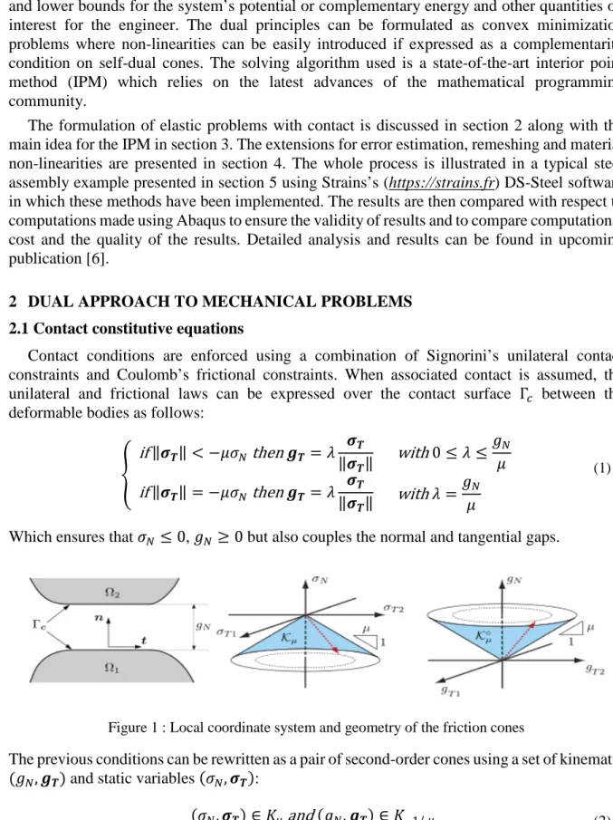
Contact conditions are enforced using a combination of Signorini’s unilateral contact constraints and Coulomb’s frictional constraints. When associated contact is assumed, the unilateral and frictional laws can be expressed over the contact surface Γ_𝑐𝑐 between the deformable bodies as follows:

� if ‖𝝈𝝈𝑻𝑻

‖<−𝜇𝜇𝜎𝜎𝑁𝑁 then 𝒈𝒈𝑻𝑻 =𝜆𝜆_{‖𝝈𝝈𝑻𝑻}𝝈𝝈𝑻𝑻_‖ with 0≤ 𝜆𝜆 ≤𝑔𝑔_𝜇𝜇𝑁𝑁

if ‖𝝈𝝈𝑻𝑻‖=−𝜇𝜇𝜎𝜎𝑁𝑁 then 𝒈𝒈𝑻𝑻 =𝜆𝜆_{‖𝝈𝝈𝑻𝑻}𝝈𝝈𝑻𝑻_‖ with 𝜆𝜆= 𝑔𝑔_𝜇𝜇𝑁𝑁

(1)

Which ensures that 𝜎𝜎_𝑁𝑁 ≤0, 𝑔𝑔𝑁𝑁≥ 0 but also couples the normal and tangential gaps.

Figure 1 : Local coordinate system and geometry of the friction cones

The previous conditions can be rewritten as a pair of second-order cones using a set of kinematic

(𝑔𝑔𝑁𝑁,𝒈𝒈𝑻𝑻) and static variables (𝜎𝜎𝑁𝑁,𝝈𝝈𝑻𝑻):

(𝜎𝜎𝑁𝑁,𝝈𝝈𝑻𝑻) ∈ 𝐾𝐾𝜇𝜇 and (𝑔𝑔𝑁𝑁,𝒈𝒈𝑻𝑻) ∈ 𝐾𝐾−1/ 𝜇𝜇

where 𝐾𝐾𝛼𝛼 = {(𝑥𝑥,𝒚𝒚)∈ ℝ×ℝ2| ‖𝒚𝒚‖+𝛼𝛼𝑥𝑥 ≤0}

3

Since 𝐾𝐾_{−1/𝜇𝜇} is the polar cone of 𝐾𝐾_𝜇𝜇, the pair of static and kinematic variables satisfies a complementarity condition over dual cones.

2.2 Energy principles as conic programs

Classical energy principles can be used to formulate finite elements problems as minimisation programs. These principles can be adapted to consider contact conditions and/or plasticity.

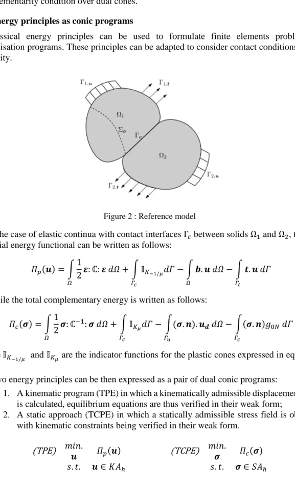
Figure 2 : Reference model

In the case of elastic continua with contact interfaces Γ_𝑐𝑐 between solids Ω₁ and Ω₂, the total potential energy functional can be written as follows:

𝛱𝛱𝑝𝑝(𝒖𝒖) =�1₂𝜺𝜺:ℂ:𝜺𝜺𝑑𝑑𝑑𝑑 𝛺𝛺 + � 𝕀𝕀𝐾𝐾_{−1/𝜇𝜇}𝑑𝑑𝑑𝑑 𝛤𝛤𝑐𝑐 − � 𝒃𝒃.𝒖𝒖𝑑𝑑𝑑𝑑 𝛺𝛺 − � 𝒕𝒕.𝒖𝒖𝑑𝑑𝑑𝑑 𝛤𝛤𝑡𝑡 (3)

While the total complementary energy is written as follows: 𝛱𝛱𝑐𝑐(𝝈𝝈) =�1₂𝝈𝝈:ℂ−𝟏𝟏_{:𝝈𝝈𝑑𝑑𝑑𝑑} 𝛺𝛺 + � 𝕀𝕀𝐾𝐾_𝜇𝜇𝑑𝑑𝑑𝑑 𝛤𝛤𝑐𝑐 − �(𝝈𝝈.𝒏𝒏).𝒖𝒖𝒅𝒅𝑑𝑑𝑑𝑑 𝛤𝛤𝑢𝑢 − �(𝝈𝝈.𝒏𝒏)𝑔𝑔0𝑁𝑁𝑑𝑑𝑑𝑑 𝛤𝛤𝑐𝑐 (4)

Where𝕀𝕀𝐾𝐾_{−1/𝜇𝜇} and 𝕀𝕀𝐾𝐾_𝜇𝜇 are the indicator functions for the plastic cones expressed in equation ( 2 ).

The two energy principles can be then expressed as a pair of dual conic programs:

1. A kinematic program (TPE) in which a kinematically admissible displacements field is calculated, equilibrium equations are thus verified in their weak form;

2. A static approach (TCPE) in which a statically admissible stress field is obtained, with kinematic constraints being verified in their weak form.

(TPE) 𝑚𝑚𝑚𝑚𝑚𝑚_𝒖𝒖 . 𝛱𝛱𝑝𝑝(𝒖𝒖) (TCPE) 𝑚𝑚𝑚𝑚𝑚𝑚_𝝈𝝈 . 𝛱𝛱𝑐𝑐(𝝈𝝈)

𝑠𝑠.𝑡𝑡. 𝒖𝒖 ∈ 𝐾𝐾𝐴𝐴ℎ 𝑠𝑠.𝑡𝑡. 𝝈𝝈 ∈ 𝑆𝑆𝐴𝐴ℎ

(5)

Indicator functions can be removed from the objective part and be passed as conic constraints obtaining then the classical from of quadratic programs.

4

Because of duality, both minimization problems provide respectively an upper and lower bound of the real potential energy of the system (after inverting the sign of the complementary energy):

−𝛱𝛱𝑐𝑐(𝝈𝝈𝒉𝒉)≤ −𝛱𝛱𝑐𝑐(𝝈𝝈∗) =𝛱𝛱𝑝𝑝(𝒖𝒖∗)≤ 𝛱𝛱𝑝𝑝(𝒖𝒖𝒉𝒉) (6) These bounds provide the engineer the capacity to judge the quality of convergence since one can evaluate the proximity of approximate solutions to the exact solution. The relative gap between the upper and lower bound therefore represents the above-introduced error estimator and serves as an excellent indicator of convergence which can be defined as:

𝛥𝛥𝛥𝛥 = 𝛱𝛱𝑝𝑝(𝒖𝒖𝒉𝒉) +𝛱𝛱𝑐𝑐(𝝈𝝈𝒉𝒉)

𝛱𝛱𝑐𝑐(𝝈𝝈𝒉𝒉) (%) (7)

3 INTERIOR POINT METHOD FOR CONIC PROGRAMS 3.1 Quadratic second-order cone programming

Both static and kinematic approaches result in a similar mathematical formulation of second-order cone programs (SOCP). These energy principles are a special case called quadratic second-order cone program (QP) which consist in minimizing a quadratic objective function under linear and conic constraints such as the positive orthant or the second order cone as shown in equation (8). 𝑚𝑚𝑚𝑚𝑚𝑚. 𝒙𝒙,𝒙𝒙𝒊𝒊 12𝒙𝒙𝑻𝑻𝑷𝑷𝒙𝒙+𝒄𝒄𝑻𝑻𝒙𝒙+𝒄𝒄𝑰𝑰𝑻𝑻𝒙𝒙𝑰𝑰 𝑠𝑠.𝑡𝑡. 𝑨𝑨𝒙𝒙𝑨𝑨𝑰𝑰𝒙𝒙 − 𝒙𝒙𝑰𝑰= 𝒃𝒃 =𝒃𝒃𝑰𝑰 𝒙𝒙𝑰𝑰∈ 𝐾𝐾 (8)

Most standard SOCP program formats assume no quadratic objective term, but the previous problem can be always reformulated as a problem involving a linear objective function only by introducing auxiliary variables and additional conic constraints [1,2,4]. However, in our implementation, the quadratic term will be kept as such in the objective function since its physical meaning is interesting.

3.2 Interior-point method solution procedure

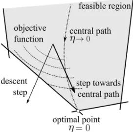
A lot of research has been carried out since the 1960s on numerical algorithms to solve optimisation problems. Today, these algorithms provide the engineer an efficient and reliable technology to solve convex programs especially SOCPs. We will focus on the primal-dual interior-point algorithm, a subclass of the interior-point methods, which is currently considered as one of the most efficient ways to solve QP problems. The idea of an IPM is to find a solution to the Karush-Kuhn-Tucker (KKT) conditions for problem (8) by following the neighbourhood of a curve called the central path and parametrized by a barrier parameter 𝜂𝜂 ≥0. The optimal solution is obtained for 𝜂𝜂 →0.

5

Figure 3: General idea of an IP algorithm

This central path is no other than the unique solution to the following perturbation of the KKT system [1,2,4].

Find (𝒙𝒙,𝒙𝒙_𝑰𝑰,𝝀𝝀,𝝂𝝂_𝑰𝑰,𝒔𝒔_𝑰𝑰) such that

𝑷𝑷𝒙𝒙+𝒄𝒄+𝑨𝑨𝑻𝑻_{𝝀𝝀+𝑨𝑨} 𝑰𝑰 𝑻𝑻_{𝝂𝝂𝑰𝑰 = 0} 𝒄𝒄𝑰𝑰− 𝝂𝝂𝑰𝑰− 𝒔𝒔𝑰𝑰 = 0 𝑨𝑨𝒙𝒙 − 𝒃𝒃 = 0 𝑨𝑨𝑰𝑰𝒙𝒙 − 𝒙𝒙𝑰𝑰− 𝒃𝒃𝑰𝑰 = 0 𝒙𝒙𝑰𝑰∘ 𝒔𝒔𝒊𝒊 = 𝜂𝜂𝒆𝒆𝑰𝑰 𝒙𝒙𝑰𝑰∈ 𝐾𝐾 ,𝒔𝒔𝑰𝑰 ∈ 𝐾𝐾∗ (9)

Where 𝒆𝒆= (1,𝟎𝟎)in the case of Lorentz cones.

The IPM relies on an iterative algorithm that calculates descent steps using Newton’s method on the residuals equations and introducing the Nesterov-Todd scaling matrices [14]. Therefore, at each iteration, a linear Newton-like system is solved:

�𝑷𝑷+𝑨𝑨𝑰𝑰𝑻𝑻𝑭𝑭𝟐𝟐𝑨𝑨𝑰𝑰 −𝑨𝑨𝑇𝑇

−𝑨𝑨 0 � �∆𝒙𝒙∆𝝀𝝀�=−𝑹𝑹 (10)

With 𝑹𝑹 being the residuals vector and 𝑭𝑭 a specific scaling matrix depending on the types of cones. After each iteration, the variables are updated to ensure that the conic constraints will always be strictly verified which ensures the verification of the physical phenomena modelled by the cones (such as non-penetration in contact pairs and plasticity cones). Considering 𝑨𝑨 of full rank, the linear system (10) is never singular, thus convergence in ensured in a limited number of iterations (ranging from 15 to 25 iterations in most cases), which is a key advantage of this method.

In comparison, incremental Newton-Raphson algorithm, based on tangent matrix and residual force, often leads to problems of convergence, especially when the initial point is “far” from the solution. Engineers must divide the loads to perform step by step analyses until a satisfactory state is calculated.

6 3.3 Finite-element discretisation

While classical quadratic 10-node displacement tetrahedra are used in the kinematic approach, special improved equilibrium elements are necessary to handle the static approach. Over a mesh made of 4-node linear tetrahedra, a “generalized” stress field, which already includes the equilibrium equation: div(𝝈𝝈) +𝒃𝒃= 0, is interpolated. This reduces the number of degrees of freedom from 6 × 4 = 24 per tetrahedra to 24−3 = 21 per tetrahedra and removes a first set of linear redundancies. Since the tetrahedra are considered disconnected, the second equilibrium equation: ⟦𝝈𝝈.𝒏𝒏⟧= 0, ensuring the continuity of the stress vector on element interfaces, should be written on all internal tetrahedron interfaces. This will cause enormous redundancies in the linear constraints matrix thus making the solved-system highly indefinite. The solution to eliminate these redundancies is to use the super-elements method introduced in [5,8] and consists in subdividing each tetrahedron into 4 and then removing all internal degrees of freedom, leaving only the ones from external faces.

4 ADVANTAGES AND EXTENSION TO MATERIAL NON-LINEARITIES 4.1 Error Estimator and remesh procedure

To limit the number of elements used in 3D analysis, a general adaptive remesh scheme is implemented using a constitutive equation type of error based on duality. This type of error qualifies, both on the local and global level, the “closeness” of the kinematic and static solutions. In short, if the gap in constitutive relation in zero, both solutions are correct and present an accurate dual representation of the optimal solution. This versatile type of error, introduced by Ladeveze [9] based on the Fenchel inequality, allows us to consider each physical phenomenon such as plasticity or contact, separately. It can be written in the case of elastic continua with contact interfaces as follows:

𝑒𝑒2_{(𝒖𝒖,𝝈𝝈) =𝑒𝑒}

𝛺𝛺2(𝒖𝒖,𝝈𝝈) +𝑒𝑒𝛤𝛤2𝑐𝑐(𝒖𝒖,𝝈𝝈) ≥0 ∀(𝒖𝒖,𝝈𝝈) (11) Which is constituted by the elastic volume part of the error and the surface contact part of the error. Thus, this error can also be expressed as:

𝑒𝑒2_{(𝒖𝒖,𝝈𝝈) =𝛱𝛱𝑝𝑝(𝒖𝒖) +𝛱𝛱𝑐𝑐(𝝈𝝈)} (12)

Therefore, the gap given by equation (12) is nothing else than a qualification of the global error and can be used to assess global convergence.

The complete procedure involves the following steps:

1. An initial static and kinematic calculation are performed over an automatically software-generated coarse mesh Ω(0);

2. On this mesh, an error calculation is made, and global, elementary and relative errors are computed along with the relative gap between objectives functions;

3. Nodal relative errors are then used to compute a new anisotropic mesh size map; 4. A new mesh Ω(1)is generated and new static and kinematic analyses are performed. The process is repeated until a target objective gap is reached.

7 4.2 An extension to material plasticity

IMP provides a reliable solution for non-linear convex problems that can be written in the form of conic problems. The most interesting part of this method is its ability to provide solutions for problems traditionally unsolvable using a Newton-Raphson procedure such as limit analysis. The use of this method is rather recent [7,10-13] and is being generalized in various yield problems in non-smooth mechanics such as viscoplastic fluids [3].

Considering material non-linearities is rather a direct extension of the dual approach exposed in this article provided that the yield condition can be written in the form of a complementarity condition over second order cones and the dissipation derives from a potential. That is the case with most standard materials, specifically steel, where a Von-Mises type plasticity can be used. The Von Mises criterion is formulated 𝑓𝑓(𝝈𝝈) =‖𝒔𝒔‖ − √2𝑘𝑘 ≤0, with 𝒔𝒔 ∈ ℝ5 the deviatoric stress tensor and 𝑘𝑘, the shear limit which can written as a second-order cone of dimension 6:

(√2𝑘𝑘,𝒔𝒔)∈ 𝐾𝐾6_.

In the case of limit analysis, the elastic response of the structure is ignored therefore the plastic failure of the structure can be analyzed. In this case, the hessian matrix is removed from the objective thus this problem is reduced to minimizing a linear term under conic constraints. It’s impossible to form a classic linear system to solve this problem, even using the incremental Newton-Raphson. Only convex optimization methods, such as interior-point algorithm, can tackle this issue.

5 EXAMPLE AND RESULTS

A typical beam-column steel assembly is used to illustrate the method. Counter-calculations are made using Abaqus finite elements software which used classical Newton-Raphson method to solve non-linear problems. To eliminate all forms of variations and to focus on the performance of the solvers only, the same series of 6 iteratively refined meshes is used in all the studies. This model is calculated using the IP algorithm and various configurations in Abaqus, corresponding to different modelling choices of contact enforcement: the penalisation (PEN) technique and the augmented Lagrangian (LA) technique.

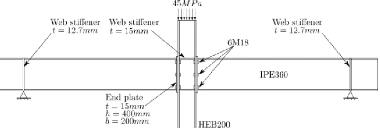
Figure 4 : Description of the model

Figure 4 gives a general description of the model. It consists of a HEB200 central column with two IPE360 beams attached over the flanges using welded end plates and bolts. The end plates have a 15𝑚𝑚𝑚𝑚thickness and 6 M18 bolts are used to attach each beam. Web stiffeners are used to prevent its buckling. For the HEB column, their thickness is 12.7𝑚𝑚𝑚𝑚to coincide with the IPE’s flange thickness, whereas for the IPE beams, 15𝑚𝑚𝑚𝑚thick stiffeners are used over the

8

supports to correctly channel shear forces. We suppose that the bolt hole is equal to its diameter and, to prevent rigid body motions, one of the bolt heads is glued to the plate. A 45𝑀𝑀𝑀𝑀𝑀𝑀 normal pressure is applied over the top section of the HEB column and the displacement of the nodes belonging to the surface defined by the intersection of the IPE’s web stiffeners are blocked in all the 3 directions, the HEB sections remaining free. All details including bolts heads and cores are modeled using 3D quadratic tetrahedrons. Material non-linearity is not considered in this example but can be included easily as discussed in section 4.

Since Abaqus offers displacement-based elements only, the calculation times are compared with respect to the kinematic approach. The solved system size is nearly the same as in Abaqus, the system sparsity patterns and conditioning are also comparable. The main difference lies in contact modelling and resolution strategy. To closely compare the numerical performance of the algorithm, all the calculations were made using the same machine. OpenMP technology was used to parallelize over 8 threads.

Table 1 : CPU times and speed-up factors of the IPM over Abaqus AL and PEN approaches Remesh

iteration Mesh size

IP kinematic approach (𝒔𝒔)(𝑵𝑵𝒊𝒊𝒕𝒕𝒆𝒆𝒊𝒊) Abaqus AL approach (𝒔𝒔)(𝑵𝑵𝒊𝒊𝒕𝒕𝒆𝒆𝒊𝒊) Speed-up factor Abaqus PEN approach (𝒔𝒔)(𝑵𝑵𝒊𝒊𝒕𝒕𝒆𝒆𝒊𝒊) Speed-up factor 0 𝑁𝑁𝑒𝑒 = 9150 10.2 (17) 25.0 (21) 2.5 9.0 (8) 0.9 1 𝑁𝑁𝑒𝑒 = 33051 28.3 (18) 69.0 (22) 2.4 30.0 (9) 1.1 2 𝑁𝑁𝑒𝑒= 42696 35.0 (17) 97.0 (24) 2.8 38.0 (9) 1.1 3 𝑁𝑁𝑒𝑒= 85187 78.8 (17) 278.0 (25) 3.5 98.0 (9) 1.2 4 𝑁𝑁𝑒𝑒 = 222082 320.6 (18) 1368.0 (30) 4.3 435.0 (10) 1.4

Table 1 shows the CPU times for the different approaches. The IPM is largely comparable to Abaqus penalty approach in terms of CPU times, with even a small speed-up factor when compared to the augmented Lagrangian approach. Compared to the latter, which generally yields more accurate results, the IPM shows a speed-up factor of 2 to 4, the speed-up factor increasing with the mesh size. This is a major advantage of the IPM since it can handle large scale sparse problems efficiently. And while Abaqus number of iterations required for convergence tends to increase (from 20 to 30 for the AL approach), the IPM number of iterations remains fairly constant varying between 18 and 20 iterations for all the remeshes.

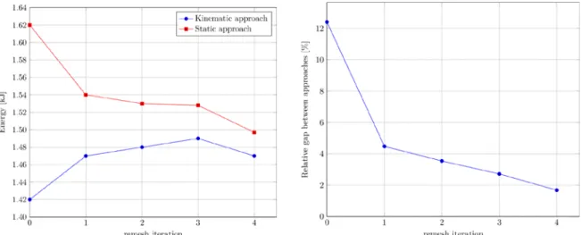
Figure 5 : Total potential and complementary energy

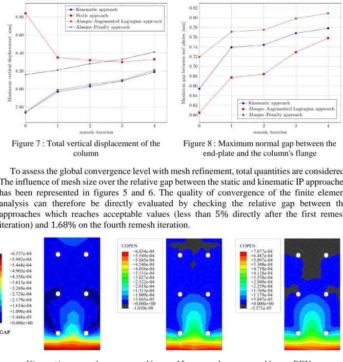
9 Figure 7 : Total vertical displacement of the

column

Figure 8 : Maximum normal gap between the end-plate and the column's flange

To assess the global convergence level with mesh refinement, total quantities are considered. The influence of mesh size over the relative gap between the static and kinematic IP approaches has been represented in figures 5 and 6. The quality of convergence of the finite element analysis can therefore be directly evaluated by checking the relative gap between the approaches which reaches acceptable values (less than 5% directly after the first remesh iteration) and 1.68% on the fourth remesh iteration.

Figure 9 : Initial mesh, gap iso-values (in m) over one of the end plates

Let us now consider some local quantities. Figure 7 shows the evolution of the total vertical displacement of the column over the six meshes. We can clearly see the upper and lower bound offered by the dual approach that we used. Abaqus AL approach shows nearly the same results as the kinematic approach whereas with the penalty contact constraints, one can easily over-estimate displacements thus leading to misinterpretations. These aspects are generally unknown to engineers who do not have means to estimate displacements from above, contrary to what offers equilibrium-based computations. The maximum gap between the end plate and the column's flange presented in figure 8 shows the consequences of the contact constraints enforcement method. With the penalty approach, the maximum gap is overestimated. An important point is that with the IPM, no contact constraint violation is permitted, thus we have zero penetration, whereas in Abaqus, a penetration tolerance is allowed. The results show that a “negative” gap, equivalent to up to 8% of the maximum gap, is possible with the penalty as

10

seen in figure 9. However, with the AL approach, negative gaps are limited to 0.0001% of the maximum gap, thus yielding better results that are comparable to the IP kinematic approach. It is clear that with the penalty approach in Abaqus and the removal of supplementary contact constraints, one can manage to obtain results in a more reasonable time.

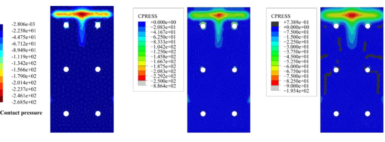
Figure 10 : Fourth remesh iteration, normal pressure iso-values (in MPa) over one of the end-plates.

Figure 10 shows the local contact pressure over the end plates, one obtained using the IP static approach and the two other from Abaqus. We can clearly see that the stresses post-processed by Abaqus from a displacement field are underestimated. While the AL approach gives slightly comparable results to the IP static approach (247𝑀𝑀𝑀𝑀𝑀𝑀 compared to 268𝑀𝑀𝑀𝑀𝑀𝑀), the penalty approach largely underestimates these values (89.2𝑀𝑀𝑀𝑀𝑀𝑀). The importance of the dual approach is clear and produces better exploitable results for engineers.

6 CONCLUSIONS

The study of a deformable continua in contact has been discussed in this article. Using a dual approach, a kinematically admissible displacement field and a statically admissible stress field can be obtained which gives the engineer more reliable results along with an error estimator and a convergence indicator. The IPM handles with no major difficulty the contact non-linearities with no user-parameter settings. The method can also be extended to consider material non-linearities such as plasticity.

Numerically, the IPMs shows stable and robust results with even better computational times as shown in the steel assembly example. The solution clearly verifies conic constraints, and this can be seen over the contact interfaces where no penetration is permitted. It also provides a better evaluation of quantities of interest for the engineer such as displacements obtained by the kinematic approach and stresses obtained by the static approach.

11 REFERENCES

[1] F. Alizadeh and D. Goldfarb, Second-order cone programming, Mathematical Programming, vol. 95, no. 1, pp. 3–51, Jan. 2003.

[2] E. D. Andersen, C. Roos, and T. Terlaky, On implementing a primal-dual interior-point method for conic quadratic optimization, Mathematical Programming, vol. 95, no. 2, pp. 249–277, Feb. 2003.

[3] J. Bleyer, Advances in the simulation of viscoplastic fluid flows using interior-point methods, Computer Methods in Applied Mechanics and Engineering, 2017.

[4] S. P. Boyd and L. Vandenberghe, Convex optimization. Cambridge, UK ; New York: Cambridge

University Press, 2004.

[5] J. P. M. De Almeida and O. J. B. A. Pereira, A set of hybrid equilibrium finite elements models for the analysis of three-dimensional solids, International Journal for Numerical Methods in Engineering, vol. 39, no. 16, pp. 2789–2802, Aug. 1996.

[6] C. El Boustani, J. Bleyer, M. Arquier, M.-K. Ferradi, and K. Sab, Dual finite-element analysis

using second-order cone programming for structures including contact, Computers & Structures

(submitted).

[7] Y. Kanno, Nonsmooth mechanics and convex optimization. Boca Raton, FL: CRC Press, 2011.

[8] M. Kempeneers, J.-F. Debongnie, and P. Beckers, Pure equilibrium tetrahedral finite elements for global error estimation by dual analysis, International Journal for Numerical Methods in Engineering, p. n/a-n/a, 2009.

[9] P. Ladevèze and J. P. Pelle, Mastering calculations in linear and nonlinear mechanics. New York: Springer Science, 2005.

[10] A. V. Lyamin and S. W. Sloan, Lower bound limit analysis using non-linear programming,

International Journal for Numerical Methods in Engineering, vol. 55, no. 5, pp. 573–611, 2002. [11] A. V. Lyamin and S. W. Sloan, Upper bound limit analysis using linear finite elements and

non-linear programming, International Journal for Numerical and Analytical Methods in Geomechanics, vol. 26, no. 2, pp. 181–216, 2002.

[12] A. Makrodimopoulos and C. M. Martin, Lower bound limit analysis of cohesive-frictional

materials using second-order cone programming, International Journal for Numerical Methods in Engineering, vol. 66, no. 4, pp. 604–634, Apr. 2006.

[13] A. Makrodimopoulos and C. M. Martin, Upper bound limit analysis using simplex strain elements and second-order cone programming, International Journal for Numerical and Analytical Methods in Geomechanics, vol. 31, no. 6, pp. 835–865, May 2007.

[14] Y. E. Nesterov and M. J. Todd, Primal-dual interior-point methods for self-scaled cones, SIAM Journal on optimization, vol. 8, no. 2, pp. 324–364, 1998.