This paper is made available online in accordance with
publisher policies. Please scroll down to view the document
itself. Please refer to the repository record for this item and our
policy information available from the repository home page for
further information.
To see the final version of this paper please visit the publisher’s website.
Access to the published version may require a subscription.
Author(s): Michał Komorowski , Bärbel Finkenstädt , Claire V Harper
and David A Rand
Article Title: Bayesian inference of biochemical kinetic parameters using
the linear noise approximation
Year of publication: 2009
Link to published version:
http://dx.doi.org/10.1186/1471-2105-10-343
Publisher statement: None
BioMedCentral
Page 1 of 10
BMC Bioinformatics
Open Access
Methodology article
Bayesian inference of biochemical kinetic parameters using the
linear noise approximation
Micha
ł
Komorowski*
1,2, Bärbel Finkenstädt
1, Claire V Harper
4and
David A Rand
2,3Address: 1Department of Statistics, University of Warwick, Coventry, UK, 2Systems Biology Centre, University of Warwick, Coventry, UK, 3Mathematics Institute, University of Warwick, Coventry, UK and 4Department of Biology, University of Liverpool, Liverpool, UK
Email: MichałKomorowski* - [email protected]; Bärbel Finkenstädt - [email protected]; Claire V Harper - [email protected]; David A Rand - [email protected]
* Corresponding author
Abstract
Background: Fluorescent and luminescent gene reporters allow us to dynamically quantify changes in molecular species concentration over time on the single cell level. The mathematical modeling of their interaction through multivariate dynamical models requires the deveopment of effective statistical methods to calibrate such models against available data. Given the prevalence of stochasticity and noise in biochemical systems inference for stochastic models is of special interest. In this paper we present a simple and computationally efficient algorithm for the estimation of biochemical kinetic parameters from gene reporter data.
Results: We use the linear noise approximation to model biochemical reactions through a stochastic dynamic model which essentially approximates a diffusion model by an ordinary differential equation model with an appropriately defined noise process. An explicit formula for the likelihood function can be derived allowing for computationally efficient parameter estimation. The proposed algorithm is embedded in a Bayesian framework and inference is performed using Markov chain Monte Carlo.
Conclusion: The major advantage of the method is that in contrast to the more established diffusion approximation based methods the computationally costly methods of data augmentation are not necessary. Our approach also allows for unobserved variables and measurement error. The application of the method to both simulated and experimental data shows that the proposed methodology provides a useful alternative to diffusion approximation based methods.
Background
The estimation of parameters in biokinetic models from experimental data is an important problem in Systems Biology. In general the aim is to calibrate the model so as to reproduce experimental results in the best possible way. The solution of this task plays a key role in interpreting experimental data in the context of dynamic
mathemati-cal models and hence in understanding the dynamics and control of complex intracellular chemical networks and the construction of synthetic regulatory circuits [1]. Among biochemical kinetic systems, the dynamics of gene expression and of gene regulatory networks are of particu-lar interest. Recent developments of fluorescent micros-copy allow us to quantify changes in protein Published: 19 October 2009
BMC Bioinformatics 2009, 10:343 doi:10.1186/1471-2105-10-343
Received: 29 January 2009 Accepted: 19 October 2009 This article is available from: http://www.biomedcentral.com/1471-2105/10/343
© 2009 Komorowski et al; licensee BioMed Central Ltd.
This is an Open Access article distributed under the terms of the Creative Commons Attribution License (http://creativecommons.org/licenses/by/2.0), which permits unrestricted use, distribution, and reproduction in any medium, provided the original work is properly cited.
concentration over time in single cells (e.g. [2,3]) even with single molecule precision (see [4] for review). There-fore an abundance of data is becoming available to esti-mate parameters of mathematical models in many important cellular systems.
Single cell imaging techniques have revealed the stochas-tic nature of biochemical reactions (see [5] for review) that most often occur far from thermodynamic equilib-rium [6] and may involve small copy numbers of reacting macromolecules [7]. This inherent stochasticity implies that the dynamic behaviour of one cell is not exactly reproducible and that there exists stochastic heterogeneity between cells. The disparate biological systems, experi-mental designs and data types impose conditions on the statistical methods that should be used for inference [8-10]. From the modeling point of view the current com-mon consensus is that the most exact stochastic descrip-tion of the biochemical kinetic system is provided by the chemical master equation (CME) [11]. Unfortunately, for many tasks such as inference the CME is not a convenient mathematical tool and hence various types of approxima-tions have been developed. The three most commonly used approximations are [12]:
1. The macroscopic rate equation (MRE) approach which describes the thermodynamic limit of the sys-tem with ordinary differential equations and does not take into account random fluctuations due to the sto-chasticity of the reactions.
2. The diffusion approximation (DA) which provides stochastic differential equation (SDE) models where the stochastic perturbation is introduced by a state dependant Gaussian noise.
3. The linear noise approximation (LNA) which can be seen as a combination because it incorporates the deterministic MRE as a model of the macroscopic sys-tem and the SDEs to approximatively describe the fluc-tuations around the deterministic state.
Statistical methods based on the MRE have been most widely studied [8,13-15]. They require data based on large populations. The main advantages of this method are its conceptual simplicity and the existence of extensive the-ory for differential equations. However, single cells exper-iments and studies of noise in small regulatory networks created the need for statistical tools that are capable to extract information from fluctuations in molecular spe-cies. Few methods used CME to address this. Algorithm, proposed by [16], approximated the likelihood function, the other, suggested by [17] simulated it using Monte Carlo methods. Recently, also a method based on the exact likelihood [18] has been developed. Although, sub-stantial progress has been made in numerical methods for
solving CME, inference algorithms based on the CME are computationally intensive and difficult to apply to prob-lems of realistic size and complexity [19]. Another group of methods is based on the DA [9,20]. This uses likelihood approximation methods (e.g. [21]) that are computation-ally intensive and require sampling from high dimen-sional posterior distributions. Inference about the volatility process becomes difficult for low frequency data that are not directly measured at the molecular level [10,20]. The aim of this study is to investigate the use of the LNA as a method for inference about kinetic parame-ters of stochastic biochemical systems. We find that the LNA approximation provides an explicit Gaussian likeli-hood for models with hidden variables and measurement error and is therefore simpler to use and computationally efficient. To account for prior information on parameters our methodology is embedded in the Bayesian paradigm. The paper is structured as follows: We first provide a description of the LNA based modeling approach and then formulate the relevant statistical framework. We then study its applicability in four examples, based on both simulated and experimental data, that clarify principles of the method. Additional file 1 contains details of mathe-matical and statistical modeling, particularly comparison of the proposed method with an algorithm based on the DA.
Methods
The chemical master equation (CME) is the primary tool to model the stochastic behaviour of a reacting chemical system. It describes the evolution of the joint probability distribution of the number of different molecular species in a spatially homogeneous, well stirred and thermally equilibrated chemical system [11].
Even though these assumptions are not necessarily satis-fied in living organisms the CME is commonly regarded as the most realistic model of biochemical reactions inside living cells. Consider a general system of N chemical spe-cies inside a volume Ω and let X = (X1,..., XN)T denote the
number and x = X/Ω the concentrations of molecules. The stoichiometry matrix S = {Sij}i = 1,2...N; j = 1,2...R describes changes in the population sizes due to R different chemi-cal events, where each Sij describes the change in the
number of molecules of type i from Xi to Xi + Sij caused by an event of type j. The probability that an event of type j occurs in the time interval [t, t + dt) equals (x, Ω, t)Ωdt. The functions (x, Ω, t) are called mesoscopic transition
rates. This specification leads to a Poisson birth and death
process where the probability h(X, t) that the system is in the state X at time t is described by the CME [12] which is given in Additional file 1. It is straightforward to verify
fj
BMC Bioinformatics 2009, 10:343 http://www.biomedcentral.com/1471-2105/10/343
Page 3 of 10 that the first order terms of a Taylor expansian of the CME
in powers of are given by the following MRE
where φi = limΩ→∞, X→∞ Xi/Ω, = ϕ(
φ
1,...,φ
N)T and.
Including also the second order terms of this expansion produces the LNA
which decomposes the state of the system into a deter-ministic part ϕas solution of the MRE in (1) and a sto-chastic process ξdescribed by an Itô diffusion equation
where W(t) denotes R dimensional Wiener process, and fi = fi(ϕ) (see Additional file 1 for derivation).
The rationale behind the expansion in terms of is that for constant average concentrations relative fluctua-tions will decrease with the inverse of the square root of volume [22]. Therefore the LNA is accurate when fluctua-tions are sufficiently small in relation to the mean (large Ω). Hence, the natural measure of adequacy of the LNA is the coefficient of variation i.e. ratio of the standard devia-tion to the mean (see Addidevia-tional file 1). Validity of this approximation is also discussed in details in [22,23]. In addition it can be shown that the process describing the deviation from the deterministic state converges weakly to the diffusion (3) as Ω→∞ [24]. In order to use the LNA in a likelihood based inference method we need to derive transition densities of the process x.
Transition densities
The LNA provides solutions that are numerically or ana-lytically tractable because the MRE in (1) can be solved numerically and the linear SDE in (3) for an initial condi-tion ξ(ti) = has a solution of the form [25]
where the integral is in the Itô sense and (s) is the fun-damental matrix of the non-autonomous system of ODEs
The Itô integral of a deterministic function is a Gaussian random variable [26], therefore equations (4), (5) imply that the transition densities of the process ξare Gaussian [26] (throughout the paper we use 'Gaussian' or 'normal' shortly to denote either a univariate or a multivariate nor-mal distribution depending on the context)
where Θ denotes a vector of all model parameters, ψ(·|μi-1, Ξi-1)
is the normal density with mean
μ
i-1 and covariance matrix Ξi-1specified by
It follows from (2) and (6) that the transition densities of x are normal
The properties of the normal distribution allow us to con-struct a convenient inference framework that is reminis-cent of the Kalman filtering methodology (see e.g. [27]).
Inference
It is rarely possible to observe the time evolution of all molecular components participating in the system of interest [28]. Therefore, we partition the process xt into those components yt that are observed and those zt that are unobserved.
Let , and
denote the time-series that comprise the values of processes x, y and z, respectively, at times t0,..., 1 / Ω d i dt S fij j t i N j R f j = = =
∑
( , ) , ,..., ; 1 1 2 (1) fj( , )j t =limΩ→∞ fj( , , )x Ω t x( )t = ( )t + ( )t − j Ω x 1 2 (2) d tx( )=A( )t xdt+E( )t dW t( ), (3) [ ( )]A t ik S fij j/ k,[ ( )]E t S f ( , )t j R ik ik k =∑
=1 ∂ ∂f = j 1 / Ω Ω12 xti x( )t t(t ti) xt t(s ti) ( )s dW s( ) , t t i i i i = − ⎛ + − ⎝ ⎜ ⎞ ⎠ ⎟ −∫
Φ Φ 1E (4) Φti d ti ds ti s ti ti I Φ Φ Φ =A( + ) , ( )0 = . (5) p(xti|xti−1, )Θ =y x( ti|mi−1,Ξi−1) (6) mi t i xt i i i i s i s i i t t t s E s − − − − − = = − = − − − 1 1 1 1 1 1 1 Φ Δ Δ Ξ Φ Φ ( ) , , ( ( ) ( ))( (tti s E s Tds t t i i − −∫
) ( )) . 1 (7) p x( ti|xti− , )= (xti | ( )ti + i , i ). − − − − 1 1 2 1 1 1 Θ y j Ω m Ω Ξ (8) x≡(xt ,...,xt ) n 0 y≡(yt0,...,ytn) z≡(zt0,...,ztn)tn. Here and throughout the paper we use the same letter to denote the stochastic process and its realization. Our aim is to estimate the vector of unknown parameters Θ from a sequence of measurements . The initial condi-tion ϕ(t0) is parameterized as an element of Θ. Given the Markov property of the process x the augmented likeli-hood P( , |Θ) is given by
where are Gaussian densities specified in (8), and is an initial density assumed to be nor-mal for mathematical convenience. It can then be shown that (see Additional file 1) is Gaussian. Therefore
where ψ(·|ϕ(t0),..., ϕ(tn), ) is Gaussian density with mean vector (ϕ(t0),..., ϕ(tn)) and covariance matrix whose elements can be calculated numerically in a straightforward way (see Additional file 1). Since the mar-ginal distributions are also Gaussian it follows that the likelihood function P( |Θ) can be obtained from the augmented likelihood (10)
where the covariance matrix Σ = {Σ(i, j)}
i, j = 0,..., n is a
sub-matrix of such that and
ϕ
y is the vector consisting of the observed components ofϕ
. Fluorescent reporter data are usually assumed to be pro-portional to the number of fluorescent molecules [29] and measurements are subject to measurement error, i.e. errors that do not influence the stochastic dynamics of the system. We therefore assume that instead of the matrix our data have the form . The param-eter λis a proportionality constant (it is straightforward to generalize for the case with different proportionality con-stants for different molecular components) and denotes a random vector for additive measurement error. For mathematical convenience we assume that the jointdistribution of the measurement error is normal with mean 0 and known covariance matrix Σε, i.e. . If measurement errors are inde-pendent with a constant variance then . Equation (11) implies that the likelihood function can be written as
Since for given data the likelihood function (12) can be numerically evaluated, any likelihood based inference is straightforward to implement. Using Bayes' theorem, the posterior distribution P(Θ| ) satisfies the relation [30]
We use the standard Metropolis-Hastings (MH) algorithm [30] to sample from the posterior distribution in (13).
Results and Discussion
In order to study the use of the LNA method for inference we have selected four examples which are related to com-monly used quantitative experimental techniques such as measurements based on reporter gene constructs and reporter assays based on Polymerase Chain Reaction (e.g. RT-PCR, Q-PCR). For expository reasons, all case studies consider a model of single gene expression.
Model of single gene expression
Although gene expression involves various biochemical reactions it is essentially modeled in terms of only three biochemical species (DNA, mRNA, protein) and four reaction channels (transcription, mRNA degradation, translation, protein degradation) [31-33]. The stoichiom-etry matrix has the form
where rows correspond to molecular species and columns to reaction channels. Let x = (r, p) denote concentrations of mRNA and protein, respectively. For the reaction rates
we can derive the following macroscopic rate equations
For the general case it is assumed that the transcription rate kR(t) is time-dependent, reflecting changes in the reg-y y z P t t xt i n i i ( , | )y z Θ = p x( |x , ) (Θp | ),Θ − =
∏
1 0 1 (9) p x( ti|xti , ) −1 Θ p x( t | ) 0 Θ x P( , | )y z Θ =y( | ( ),..., ( ), ),x j t0 j tn Σ (10) ˆ Σ ˆ Σ y P( | )y Θ =y( |y jy( ),...,t0 jy( )), ),tn Σ (11) ˆ Σ Σ( , )i j ( , ) t t Cov i j = y y y u≡ly+(t ,...,t ) n 0 t i (t ,...,t ) ~ ( , ) n N 0 0Σ s2 Σ =s2I P( | )u Θ =y( | (u l jy( ),...,t0 jy( )),tn l2Σ Σ+ ). (12) u u P( | )Θ u ∝P( | ) ( ).u Θp Θ (13) S= − − ⎛ ⎝ ⎜ ⎞ ⎠ ⎟ 1 1 0 0 0 0 1 1 , (14) f x( )=(k tR( ),gRr k r, P ,gPp)T (15) fR =k tR( )−g fR R, fP =kP Rf −g fP P. (16)BMC Bioinformatics 2009, 10:343 http://www.biomedcentral.com/1471-2105/10/343
Page 5 of 10 ulatory environment of the gene such as the availability of
transcription factors or chromatin structure.
Using (14), (15) and (16) in (3) we obtain the following SDEs describing the deviation from the macroscopic state (see section 3.1.4 of Additional file 1 for derivation)
We will refer to the model in (16) and (17) as the simple
model of single gene expression.
In order to test our method on a nonlinear system we will also consider the case of an autoregulated network where the transcription rate of the gene is a function of the con-centration of the protein that the gene codes for and where the protein is a transcription factor that inhibits the production of its own mRNA. This is parameterized by a
Hill function [31] where
kR(t) now describes the maximum rate of transcription, H is a dissociation constant and nH is a Hill coefficient.
Thus, the nonlinear autoregulatory model the system is described by the MRE
and the SDEs
where . We refer to this model as
the autoregulatory model of single gene expression. The two
models constitute the basis of our inference studies below.
Inference from fluorescent reporter gene data for the simple model of single gene expression
To test the algorithm we first use the simple model of sin-gle gene expression. We generate data according to the sto-ichiometry matrix (14) and rates (15) using Stochastic Simulation Algorithm (SSA) [34] and sample it at discrete time points. We then generate artificial data that are pro-portional to the simulated protein data with added nor-mally distributed measurement error with known variance . Furthermore we assume that mRNA levels are unobserved. The volume of the system Ω is unknown
and we put Ω = 1 so that concentration equals the number of molecules. Thus the data are of the form
where is the simulated protein concen-tration, λis an unknown proportionality constant and is measurement error. For the purpose of our example we model the transcription function by
This form of transcription corresponds to an experiment, where transcription increases for t ≤b3 as a result of being induced by an environmental stimulus and for t > b3 decreases towards a baseline level b4.
We assume that at time t0 (t0 <<b3) the system is in a
sta-tionary state. Therefore, the initial condition of the MRE is a function of unknown parameters (
ϕ
R(t0),ϕ
P(t0)) = (b4/γR, b4kP/γRγP).
To ensure identifiability of all model parameters we assume that informative prior distributions for both deg-radation rates are available. Priors for all other parameters were specified to be non-informative. To infer the vector of unknown parameters
we sample from the posterior distribution
using the standard MH algorithm. The distribution P( |Θ) is given by (12).
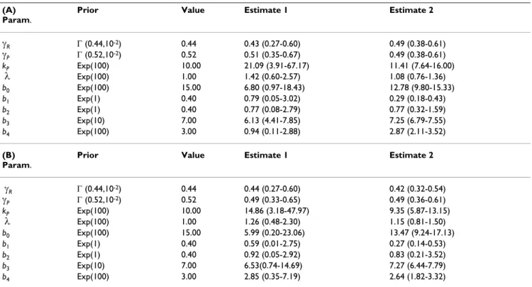
The protein level of the simulated trajectory is sampled every 15 minutes and a sample size of 101 points obtained. We perform inference for two simulated data sets: estimate 1 is based on a single trajectory while esti-mate 2 represents a larger data set using 20 sampled trajec-tories (see Figure 1A). All prior specifications, parameters used for the simulations and inference results are pre-sented in Table 1A. Estimate 1 demonstrates that it is pos-sible to infer all parameters from a single, short length time series with a realistically achievable time resolution. Estimate 2 shows that usage of the LNA does not seem to result in any significant bias. A bias has not been detected despite the very small number of mRNA molecules (5 to 35 - Figure 2A in Additional file 1) and protein molecules (100 to 500 - Figure 1A). The coefficient of variation
var-d dt k t t dW d k dt k t R R R R R R R P P R P P P R P P x g x g f x x g x f g f = − + + = − + + ( ) ( ) ( ) ( ) (( )t dWP. (17) k t pR( , )=k tR( ) /(1+( /p H)nH fR =k tR( ,fP)−g fR R, fP =kP Rf −g fP P (18) d k t dt k t t dW d k dt k R R P R R R R R R P P R P P P x x g x g f x x g x f = ′ − + + = − + ( ) ) ( ) ( ) ( ) RR( )t +g fP P( )t dWP (19) ′ ≡ ∂ ∂ k tR( ) k tR( ,fP) / fP s2 u=(ut0,...,utn) ,T (20) ut pt t pt i =l i +i, i t i k t b b t b b t b b b t b b t b R( ) exp( ( ) ) exp( ( ) ) . = − − + ≤ − − + > ⎧ ⎨ ⎪ 0 1 3 2 4 3 0 2 3 2 4 3 ⎩⎩⎪ (21) Θ =(gR,gP,kP, ,l b b b b b0, 1, 2, 3, 4) P( | )Θ u ∝P( | ) ( )u Θp Θ u
ied between approximately 0.15 and 0.4 for both molecu-lar species (Figure 1 in the Additional file 1).
Inference for this model required sampling from the 9 dimensional posterior distribution (number of unknown parameters). If instead one used a diffusion approxima-tion based method it would be necessary to sample from a posterior distribution of much higher dimension (see Additional file 1). In addition, incorporation of the meas-urement error is straightforward here, whereas for other methods it involves a substantial computational cost [20].
Inference from fluorescent reporter gene data for the model of single gene expression with autoregulation
The following example considers the autoregulatory sys-tem with only a small number of reacting molecules. Using SSA we generated artificial data from the single gene expression model with autoregulation. The protein time
courses were then sampled every 15 minutes at 101 dis-crete points per trajectory (see Figure 1B). As before we assume that the mRNA time courses are not observed and that the protein data are of the form given in (20), i.e. pro-portional to the actual amount of protein with additive Gaussian measurement error. As in the previous case study we estimate parameters from two simulated data sets, a single trajectory and an ensemble of 20 independ-ent trajectories. The inference results summarized in Table 1B show that despite the low number of mRNA (0-15 molecules, see Figure 2 in Additional file 1) and protein (10-250 molecules, see Figure B) all parameters can be estimated well with appropriate precision.
Inference for PCR based reporter data
In the case of reporter assays based on Polymerase Chain Reaction (e.g. RT-PCR, Q-PCR) measurements are obtained from the extraction of the molecular contents Protein timeseries generated using Gillespie's algorithm for the simple A and autoregulatory B models of single gene expres-sion with added measurement error ( = 9)
Figure 1
Protein timeseries generated using Gillespie's algorithm for the simple A and autoregulatory B models of sin-gle gene expression with added measurement error ( = 9). Initial conditions for mRNA and protein were sampled from Poisson distributions with means equal to the stationary means of the system with equal constant transcription rate b4. In the autoregulatory case we set H = b4kP/2γRγP. In each panel 20 time series are presented. The deterministic and average trajec-tories are plotted in bold black and red lines respectively. Corresponding mRNA trajectrajec-tories (not used for inference) are pre-sented in Additional file 1.
0 5 10 15 20 25 100 200 300 400 500 600 time
fluorescence intensity (arbitrary units)
A
0 5 10 15 20 25 0 5 0 100 150 200 250 timefluorescence intensity (arbitrary units)
B
s
BMC Bioinformatics 2009, 10:343 http://www.biomedcentral.com/1471-2105/10/343
Page 7 of 10 from the inside of cells. Since the sample is sacrificed, the
sequence of measurements are not strictly associated with a stochastic process describing the same evolving unit. Assume that at each time point ti (i = 0,..n) we observe l measurements that are proportional to the number of RNA molecules either from a single cell or from a popula-tion of s cells. This gives a (n + 1) × l matrix of data points
where is the actual RNA level, λ is the proportionality constant, is a Gaussian independ-ent measuremindepend-ent error indexed by time ti. j = 1,..., l indexes the l measurements that are taken at time ti. Note that and are independent random variables as they refer to different cells. We assume that the dynamics
of RNA is described by the simple model of single gene expression with LNA equations (16) and (17). Let ϒt
denote the distribution of measured RNA at time t (ut ~ ϒt). In order to accommodate for the different form of data we modify the estimation procedure as follows. For analytical convenience we assumed that the initial distri-bution is normal . This together with eq. (8) and normality of measurement error implies that
. Simple explicit formulae for μt and are derived in Additional file 1. Since all observations are independent we can write the posterior distribution as u≡{ut j ii,}=0,... ;n j=1,...,.l (22) ut j rt j t j rt j i, =l i, +i,, i, t j i, rt ji, rti+1,j ϒt0 N ut0 t0 2 = ( ,s ) ϒt =N u( ,t st2) st2 ut i p( | )Θ u ∝ y( , |m ,s ) ( ),p Θ = =
∏
∏
ut j t t j l i n i i i 2 1 0 (23) Left: PCR based reporter assay data simulated with Gillespie's algorithm using parameters presented in Table 2 and extracted 51 times (n = 50), every 30 minutes with an independently and normally distributed error ( = 9)Figure 2
Left: PCR based reporter assay data simulated with Gillespie's algorithm using parameters presented in Table 2 and extracted 51 times (n = 50), every 30 minutes with an independently and normally distributed error ( = 9). Each cross correspond to the end of simulated trajectory, so that the data drawn are of form (22). Since number of RNA molecules is know upto proportionality constant y-axis is in arbitrary units. Time on x-axis is expressed in hours. Estimates inferred form this data are shown in column Estimate 1 in Table 2. Right: Fluorescence level from cycloheximide experiment is plotted against time (in hours). Subsequent dots correspond to measurements taken every 6 minutes.
+ + + ++ + + + + + + + + + + + + + + + + + + ++ + ++ + + + + ++ + ++ + ++ ++ + ++ + + + + + + 0 5 10 15 20 25 0 5 10 15 20 25 30 35 time (hours)
RNA concentration (arbitrary units)
+ ++ + + + + + + + + + + + + ++ + + + + +++ + + + + + ++ + + + + + + + + + + ++ + + ++ + + + + + + + ++ + ++ + +++ + + + + + + + + ++ ++ + + + + + + + + + + + + + + + + + + + + + + + + + + + + + + + + +++ + + ++ + ++ + + + + + + + + + + + + + +++ ++ + + + ++ + ++ + + + + + + + + + + + + + +++ ++ + + + ++ + + + + + +++ + ++ + + + ++ + + + + ++ + + ++ ++ + + + ++ + + ++ + + + + + + + + + + + + + + + + + + + + + + + + + + ++ + + + + +++ + +++ + + ++ + + ++ + + + + + + + + + + + + + + + + + + + + + + + + + + + + + + + + + + + + + + + + + + ++ + + + + + + + + + + ++ + +++ + + + + + + + ++ + + + + ++ + + ++ + ++ + + + + + ++ + + + + + + + + + + +++ + ++++ +++ + + + + + + + + + + + + + ++ + + + + + + + + + + + + + + + + + + + + + + ++ ++ + + + + + + + ++ + + + +++ ++ ++ + + + + + + + + ++ + + + ++ + + ++ + + + ++ + + + + + + + + + + +++ + + 2 4 6 8 10 12 14 0 200 400 600 800 time (hours)
fluorescence intensity (arbitrary units)
where ψ(·| , ) is the normal density with parame-ters , . In order to infer the vector of the unknown parameters Θ = (γR, λ, b0, b1, b2, b3, b4, , ) we
sam-ple from the posterior using a standard MH algorithm. To test the algorithm we have simulated a small (l = 10, n = 50, plotted in Figure 2) and a large (l = 100, n = 50) data set using SSA algorithm with parameter values given in Table 2. The data were sampled discretely every 30
min-utes and a standard normal error was added. Initial condi-tions were sampled from the Poisson distribution with mean b4/γR. The estimation results in Table 2 show that parameters can be inferred well in both cases even though the number of RNA molecules in the generated data is very small (about 5-35 molecules). Since subsequent measurements do not belong to the same stochastic trajec-tory, estimation for the model presented here is not straightforward with the diffusion approximation based methods. uti sti 2 uti st2i ut0 st0 2
Table 1: Inference results for (A) the simple model and (B) autoregulatory model of single gene expression
(A) Param.
Prior Value Estimate 1 Estimate 2
γR Γ (0.44,10-2) 0.44 0.43 (0.27-0.60) 0.49 (0.38-0.61) γP Γ (0.52,10-2) 0.52 0.51 (0.35-0.67) 0.49 (0.38-0.61) kP Exp(100) 10.00 21.09 (3.91-67.17) 11.41 (7.64-16.00) λ Exp(100) 1.00 1.42 (0.60-2.57) 1.08 (0.76-1.36) b0 Exp(100) 15.00 6.80 (0.97-18.43) 12.78 (9.80-15.33) b1 Exp(1) 0.40 0.79 (0.05-3.02) 0.29 (0.18-0.43) b2 Exp(1) 0.40 0.77 (0.08-2.79) 0.77 (0.32-1.59) b3 Exp(10) 7.00 6.13 (4.41-7.85) 7.25 (6.79-7.55) b4 Exp(100) 3.00 0.94 (0.11-2.88) 2.87 (2.11-3.52) (B) Param.
Prior Value Estimate 1 Estimate 2
γR Γ (0.44,10-2) 0.44 0.44 (0.27-0.60) 0.42 (0.32-0.54) γP Γ (0.52,10-2) 0.52 0.49 (0.33-0.65) 0.49 (0.36-0.61) kP Exp(100) 10.00 14.86 (3.18-47.97) 9.35 (5.87-13.15) λ Exp(100) 1.00 1.26 (0.48-2.30) 1.15 (0.81-1.50) b0 Exp(100) 15.00 5.99 (0.20-23.06) 13.47 (9.24-17.13) b1 Exp(1) 0.40 0.59 (0.01-2.75) 0.27 (0.14-0.53) b2 Exp(1) 0.40 0.92 (0.05-2.92) 0.83 (0.21-3.52) b3 Exp(10) 7.00 6.53(0.74-14.69) 7.27 (6.44-7.79) b4 Exp(100) 3.00 2.85 (0.35-7.19) 2.64 (1.82-3.32)
Parameter values used in simulation, prior distribution, posterior medians and 95% credibility intervals. Estimate 1 corresponds to inference from single time series, Estimate 2 relates to estimates obtained from 20 independent time series. Data used for inference are plotted in Figure A for case A and Figure B for case B. Variance of the measurement error was assumed to be known = 9. Rates are per hour. Parameters are nH = 1, H = 61.98 in case B.
Table 2: Inference results for PCR based reporter assay simulated data
Parameter Prior Value Estimate 1 Estimate 2
γR Exp(1) 0.44 0.45 (0.35-0.60) 0.46 (0.42-0.50) λ Exp(100) 1.00 1.07 (0.90-1.22) 1.01 (0.95-1.05) b0 Exp(100) 15.00 13.13 (10.20-15.87) 14.91 (13.86-15.77) b1 Exp(1) 0.40 0.29 (0.14-0.51) 0.43 (0.32-0.54) b2 Exp(1) 0.40 0.32 (0.12-0.93) 0.32 (0.21-0.43) b3 Exp(10) 7.00 7.05 (6.39-7.63) 6.99 (6.76-7.15) b4 Exp(100) 3.00 2.97 (2.00-4.18) 3.10 (2.76-3.43) 0 Exp(100) 6.76 6.90 (5.79-7.69) 6.55 (6.14-6.85) Exp(100) 6.76 3.52 (0.01-8.99) 7.59 (5.44-9.49)
Parameter values used to generate data, prior distributions used for estimation, posterior median estimates together with 95% credibility intervals. Estimate 1, Estimate 2 columns relate to small (l = 5, n = 50) and large (l = 100, n = 50) sample sizes. Variance of the measurement was assumed to be known = 4. Estimated rates are per hour.
s02
BMC Bioinformatics 2009, 10:343 http://www.biomedcentral.com/1471-2105/10/343
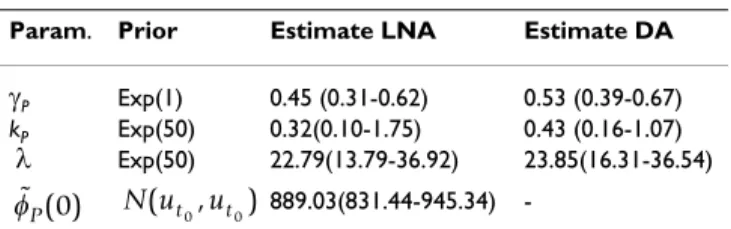
Page 9 of 10 Estimation of gfp protein degradation rate from
cycloheximide experiment
In this section the method is applied to experimental data. After a period of transcriptional induction, translation of gfp was blocked by the addition of cycloheximide (CHX). Details of the experiment are presented in Additional file 1. Fluorescence was imaged every 6 minutes for 12.5 h (see Figure 2). Since inhibition may not be fully efficient we assume that translation may be occurring at a (possibly small) positive rate kP. The model with the LNA is
The observed fluorescence is assumed to be proportional to the signal with proportionality constant λ. For compar-ison we also consider the diffusion approximation for which an exact transition density can be derived analyti-cally (see Additional file 1 for derivation)
Since incorporation of measurement error for the diffu-sion approximation based model is not straightforward, we assume that measurements were taken without any error to ensure fair comparison between the two approaches. Table 3 shows that estimates obtained with both methods are not very different.
Conclusion
The aim of this paper is to suggest the LNA as a useful and novel approach to the inference of biochemical kinetics parameters. Its major advantage is that an explicit formula for the likelihood can be derived even for systems with unobserved variables and data with additional measure-ment error. In contrast to the more established diffusion approximation based methods [9,20] the computation-ally costly methods of data augmentation to approximate transition densities and to integrate out unobserved model variables are not necessary. Furthermore, this
method can also accommodate measurement error in a straightforward way.
The suggested procedure here is implemented in a Baye-sian framework using MCMC simulation to generate pos-terior distributions. The LNA has previously been studied in the context of approximating Poisson birth and death processes [22-24,35] and it was shown that for a large class of models the LNA provides an excellent approxima-tion. Furthermore, in [35] it is shown that for the systems with linear reaction rates the first two moments of the transition densities resulting from the CME and the LNA are equal. Here we propose using the LNA directly for inference and provide evidence that the resulting method can give very good results even if the number of reacting molecules is very small. In our previous study [10] we have presented differences between fitting deterministic and stochastic models, where we used diffusion approxi-mation based method. Our experience from that work and from study [20] is that implementation of diffusion approximation based methods is challenging especially for data that are sparsely sampled in time because the need for imputation of unobserved time points leads to a very high dimensionality of the posterior distribution. This usually results in highly autocorrelated traces affect-ing the speed of convergence of the Markov chain. Our method considerably reduces the dimension of the poste-rior distribution to the number of unknown parameters of a model only and is independent of the number of unob-served components (see Additional file 1). Nevertheless it can only be applied to the systems with sufficiently large volume, where fluctuations around a deterministic state are relatively close to the mean.
Authors' contributions
MK proposed and implemented the algorithm. CVH per-formed the cycloheximide experiment. MK wrote the paper with assistance from BF and DAR, who supervised the study.
Additional material
Acknowledgements
This research was funded by BBSRC SABR grant BB/F005814/1 and EU BIOSIM Network Contract 005137. DAR is funded by EPSRC Senior
f g f x g f g f P P P P P P P P P P P k d dt k dW = − = − + + , . (24) dp=(kP−gPp dt) + kP+gPpdWP. (25)
Additional file 1
Supplemental information. Supplementary information contains deriva-tion of the theoretical results, details about algorithm implementaderiva-tion and comparison with the inference method based on the diffusion approxima-tion.
Click here for file
[http://www.biomedcentral.com/content/supplementary/1471-2105-10-343-S1.PDF]
Table 3: Inference results for CHX experimental data
Param. Prior Estimate LNA Estimate DA
γP Exp(1) 0.45 (0.31-0.62) 0.53 (0.39-0.67)
kP Exp(50) 0.32(0.10-1.75) 0.43 (0.16-1.07)
λ Exp(50) 22.79(13.79-36.92) 23.85(16.31-36.54) 889.03(831.44-945.34)
-Priors, posterior mean and 95% credibility intervals obtained from CHX experimental data using the LNA approach and diffusion approximation approach. Estimation with the LNA involved one more parameter . Estimated rates are per hour.
fP( )0 N u( t0,ut0)
Publish with BioMed Central and every scientist can read your work free of charge "BioMed Central will be the most significant development for disseminating the results of biomedical researc h in our lifetime."
Sir Paul Nurse, Cancer Research UK
Your research papers will be:
available free of charge to the entire biomedical community peer reviewed and published immediately upon acceptance cited in PubMed and archived on PubMed Central yours — you keep the copyright
Submit your manuscript here:
http://www.biomedcentral.com/info/publishing_adv.asp
BioMedcentral
Research Fellowship EP/C544587/1 and MK by studentship, Dept of Statis-tics, University of Warwick. CVH was funded by Wellcome Trust Pro-gramme Grant (067252, to JRED and MRHW) and now is recipient of The Prof. John Glover Memorial Postdoctoral Fellowship.
References
1. Ehrenberg M, Elf J, Aurell E, Sandberg R, Tegner J: Systems Biology Is Taking Off. Genome Res 2003, 13(11):2377-2380.
2. Elowitz MB, Levine AJ, Siggia ED, Swain PS: Stochastic Gene Expression in a Single Cell. Science 2002, 297(5584):1183-1186. 3. Nelson DE, Ihekwaba AEC, Elliott M, Johnson JR, Gibney CA, et al.:
Oscillations in NF-kappaB Signaling Control the Dynamics of Gene Expression. Science 2004, 306(5696):704-708. 4. Xie SX, Choi PJ, Li GW, Lee NK, Lia G: Single-Molecule
Approach to Molecular Biology in Living Bacterial Cells.
Annual Review of Biophysics 2008, 37:417-444.
5. Raser JM, O'Shea EK: Noise in Gene Expression: Origins, Con-sequences, and Control. Science 2005, 309(5743):2010-2013. 6. Keizer J: Statistical Thermodynamics of Nonequilibrium Processes
Springer, New York; 1987.
7. Guptasarma P: Does replication-induced transcription regu-late synthesis of the myriad low copy number proteins of Escherichia coli? Bioessays 1995, 17(11):987-97.
8. Moles CG, Mendes P, Banga JR: Parameter Estimation in Bio-chemical Pathways: A Comparison of Global Optimization Methods. Genome Res 2003, 13(11):2467-2474.
9. Golightly A, Wilkinson DJ: Bayesian Inference for Stochastic Kinetic Models Using a Diffusion Approximation. Biometrics 2005, 61(3):781-788.
10. Finkenstadt B, Heron E, Komorowski M, Edwards K, Tang S, Harper C, Davis J, White M, Millar A, Rand D: Reconstruction of tran-scriptional dynamics from gene reporter data using differen-tial equations. Bioinformatics 2008, 24(24):2901.
11. Gillespie DT: A Rigorous Derivation of the Chemical Master Equation. Physica A 1992, 188(1-3):404-425.
12. Van Kampen N: Stochastic Processes in Physics and Chemistry. North Hol-land 2006.
13. Mendes P, Kell D: Non-linear optimization of biochemical pathways: applications to metabolic engineering and param-eter estimation. Bioinformatics 1998, 14(10):869-883.
14. Ramsay JO, Hooker G, Campbell D, Cao J: Parameter estimation for differential equations: a generalized smoothing approach. Journal of the Royal Statistical Society: Series B (Statistical Methodology) 2007, 69(5):741-796.
15. Esposito W, Floudas C: Global Optimization for the Parameter Estimation of Differential-Algebraic Systems. Industrial and Engineering Chemistry Research 2000, 39(5):1291-1310.
16. Reinker S, Altman R, Timmer J: Parameter estimation in sto-chastic biochemical reactions. Systems Biology, IEE Proceedings 2006, 153(4):168-178.
17. Tian T, Xu S, Gao J, Burrage K: Simulated maximum likelihood method for estimating kinetic rates in gene expression. Bio-informatics 2007, 23:84.
18. Boys R, Wilkinson D, Kirkwood T: Bayesian inference for a dis-cretely observed stochastic kinetic model. Statistics and Com-puting 2008, 18(2):125-135.
19. Wilkinson D: Stochastic modelling for quantitative descrip-tion of heterogeneous biological systems. Nature Reviews Genet-ics 2009, 10(2):122-133.
20. Heron EA, Finkenstadt B, Rand DA: Bayesian inference for dynamic transcriptional regulation; the Hes1 system as a case study. Bioinformatics 2007, 23(19):2596-2603.
21. Elerian O, Chib S, Shephard N: Likelihood Inference for Dis-cretely Observed Nonlinear Diffusions. Econometrica 2001,
69(4):959-993.
22. Elf J, Ehrenberg M: Fast Evaluation of Fluctuations in Biochem-ical Networks With the Linear Noise Approximation.
Genome Res 2003, 13(11):2475-2484.
23. Lars F, Per L, Andreas H: A Hierarchy of Approximations of the Master Equation Scaled by a Size Parameter. Journal of Scien-tific Computing 2007, 34(2):127-151.
24. Kurtz TG: The Relationship between Stochastic and Deter-ministic Models for Chemical Reactions. The Journal of Chemical Physics 1972, 57(7):2976-2978.
25. Arnold L: Stochastic differential equations: theory and applications Wiley-Interscience; 1974.
26. Oksendal B: Stochastic differential equations: an introduction with applica-tions 3rd edition. Springer; 1992.
27. Brockwell P, Davis R: Introduction to time series and forecasting Springer New York; 2002.
28. Ronen M, Rosenberg R, Shraiman BI, Alon U: Assigning numbers to the arrows: Parameterizing a gene regulation network by using accurate expression kinetics. Proceedings of the National Academy of Sciences of the United States of America 2002,
99(16):10555-10560.
29. Wu JQ, Pollard TD: Counting Cytokinesis Proteins Globally and Locally in Fission Yeast. Science 2005, 310(5746):310-314. 30. Gamerman D, Lopes HF: Markov Chain Monte Carlo Stochastic
Simula-tion for Bayesian Inference 2nd ediSimula-tion. Chapman & Hall/CRC; 2006. 31. Thattai M, van Oudenaarden A: Intrinsic noise in gene regulatory
networks. Proceedings of the National Academy of Sciences 2001. 151588598
32. Chabot JR, Pedraza JM, Luitel P, van Oudenaarden A: Stochastic gene expression out-of-steady-state in the cyanobacterial circadian clock. Nature 2007, 450:1249-1252.
33. Komorowski M, Miekisz J, Kierzek A: Translational Repression Contributes Greater Noise to Gene Expression than Tran-scriptional Repression. Biophysical Journal 2009, 96(2):. 34. Gillespie DT: Exact stochastic simulation of coupled chemical
reactions. Journal of Physical Chemistry 1977, 81(25):2340-2361. 35. Ryota T, Hidenori K, J KT, Kazuyuki A: Multivariate analysis of
noise in genetic regulatory networks. Journal of Theoretical Biol-ogy 2004, 229(4):501-521.