Article
Workflow for Data Analysis in Experimental and
Computational Systems Biology: Using Python
as ‘Glue’
Melinda Badenhorst† , Christopher J. Barry† , Christiaan J. Swanepoel† ,
Charles Theo van Staden†, Julian Wissing†and Johann M. Rohwer *
Laboratory for Molecular Systems Biology, Department of Biochemistry, Stellenbosch University, Stellenbosch 7600, South Africa
* Correspondence: [email protected]; Tel.:+27-21-808-5843 † These authors contributed equally to this work.
Received: 10 June 2019; Accepted: 11 July 2019; Published: 18 July 2019
Abstract:Bottom-up systems biology entails the construction of kinetic models of cellular pathways
by collecting kinetic information on the pathway components (e.g., enzymes) and collating this into
a kinetic model, based for example on ordinary differential equations. This requires integration
and data transfer between a variety of tools, ranging from data acquisition in kinetics experiments, to fitting and parameter estimation, to model construction, evaluation and validation. Here, we present a workflow that uses the Python programming language, specifically the modules from the SciPy stack, to facilitate this task. Starting from raw kinetics data, acquired either from spectrophotometric assays with microtitre plates or from Nuclear Magnetic Resonance (NMR) spectroscopy time-courses, we demonstrate the fitting and construction of a kinetic model using scientific Python tools. The analysis takes place in a Jupyter notebook, which keeps all information related to a particular experiment together in one place and thus serves as an e-labbook, enhancing reproducibility and traceability. The Python programming language serves as an ideal foundation for this framework because it is powerful yet relatively easy to learn for the non-programmer, has a large library of scientific routines and active user community, is open-source and extensible, and many computational systems biology software tools are written in Python or have a Python Application Programming Interface (API). Our workflow thus enables investigators to focus on the scientific problem at hand rather than worrying about data integration between disparate platforms.
Keywords: enzyme kinetics; Jupyter notebook; kinetic modelling; Matplotlib; NMR spectroscopy;
optimisation; parametrisation; PySCeS; SciPy; validation
1. Introduction
With the inexorable advance of experimental techniques, the workload of researchers has begun shifting from data generation to data processing and analysis. Accordingly, it will become increasingly important for the systems biologist in the laboratory to utilise computational methods to improve data processing and visualisation of results. Computational systems biology presents the researcher with a powerful toolbox to integrate large kinetic datasets into models and eventually high resolution
analyses of biological systems [1]. The rationale for applying the systems approach to studying living
cells is that the effects of dynamically interacting macromolecules can often only be understood in
the context of complete systems (e.g., signalling networks or metabolic pathways); unintuitive and emergent properties would be missed if the macromolecules were studied in a reductionist and
decontextualised manner without considering their interactions [2].
Two opposite approaches of biological model development have emerged, termed ‘top-down’ and ‘bottom-up’. The bottom-up approach involves assembling a collection of smaller systems into a more complex system. Bottom-up kinetic models are both mechanistic and dynamic and are capable of
steady state and time-course simulations [3]. In contrast to this, the top-down approach often involves
constraint-based descriptive modelling where large datasets are used to infer relationships between
parameters without necessarily understanding the underlying mechanisms [4].
Bottom-up systems biology principally involves the construction of kinetic models,
their parametrisation and finally validation [4]. The system components are characterised in
detail in terms of formulation of mathematical relationships that quantify the dependence of each component on species that it interacts with (in the case of enzymes, these would be enzyme-kinetic
rate equations, see, e.g., [5,6]). Kinetic parameters for the rate equations are obtained from literature or
from experimental studies. Ultimately, these constituent descriptions are integrated into a combined
kinetic model in order to describe the whole system from the bottom up [4].
Kinetic models are constructed as a series of reactions that are linked in a stoichiometric network,
with each reaction described by an appropriate rate equation (reviewed, e.g., in [7]). These are then
integrated into a series of ordinary differential equations (ODEs) describing the rates of change of
the variable species (typically metabolites) [8]. Systems of ODEs can be integrated to track changes
in species concentrations and reaction rates over time, or solved for steady state using appropriate
solvers. Once a model has been constructed and sufficiently parametrised, the system can be simulated
under a range of different conditions, which can be used to discover non-intuitive system properties or
to compare different models of the same system [9]. All of these analyses require close integration
between the simulation software and experimental datasets.
The foundation of the bottom-up systems biology approach is provided by kinetic parameters, which need to be determined for each enzyme in the pathway investigated. One of the most routine analyses is therefore model fitting for parameter estimation by iteratively minimising the sum of
squares of the differences between model and experimental data [9]. Classically, these parameters
are obtained with spectrophotometric assays to determine initial reaction rates [10]. This low-cost
technique is well established and measures the progress of a reaction by monitoring the change in a light-absorbing species over time; these assays are frequently miniaturised and the throughput increased by making use of microtitre plates. Enzyme-kinetic parameters for the substrates and
products are determined by fitting a kinetic rate equation to datasets of initial rateversusconcentration.
As a second alternative, if no convenient spectrophotometric assay is available, metabolites
can also be measured with (high performance) liquid chromatography [11], either on its own, e.g.,
using detection by UV-light absorbance, or in combination with mass spectrometry. In contrast to spectrophotometric measurements, this is a discontinuous assay, requiring that the reaction be
quenched at different time points before the substrates and products are analysed in order to obtain
a time-course.
A third method involves using Nuclear Magnetic Resonance (NMR) spectroscopy to follow the progress curve of a reaction or reactions by measuring the concentrations of substrates and products
on-line in a non-invasive way. Various time-courses with different initial conditions are then fitted to a
kinetic model to obtain kinetic parameters for the enzymes [12].
In this paper we describe a simple workflow for bridging the gap between experimental and
computational systems biology using the Python programming language (http://python.org). We show
that Python is well suited to performing the computational analyses required for experimental data processing, fitting of enzyme-kinetic parameters, construction of kinetic models, as well as model validation and further analysis. More specifically, the methods will elaborate on how to construct kinetic models using the principles of bottom-up systems biology, to fit the model to experimental data and do validation runs to further test the accuracy of the model. In this way, we showcase Python and its associated software packages as a ‘glue’ that can assist the investigator with integration and simultaneous processing of numerous datasets.
2. Methods
2.1. Python Libraries and Applications
This section provides a description of the Python modules that were used to assemble the workflow. Python has many excellent and well-maintained libraries that facilitate high-level scientific computing analyses. The following libraries were used in this work (references listed provide further information and documentation):
• numpy[13], a numerical processing library that supports multi-dimensional arrays;
• scipy [14], a scientific processing library providing advanced tools for data analysis,
including regression, ODE solvers and integrators, linear algebra and statistical functions; • pandas[15], a data and table manipulation library that offers similar functionality to spreadsheets
such as Excel; and
• matplotlib[16], a plotting library with tools to display data in a variety of ways.
These libraries, plus a host of others for data science, can be downloaded as a pre-packaged
bundle from various distributions, such as the Anaconda Software Distribution [17], which is freely
available for Windows, macOS and Linux. This makes installation of the pre-requisites a simple task.
2.1.1.PySCeS
To model metabolic pathways, we used the open-source Python Simulator for Cellular Systems, PySCeS[18], which was developed in our group to simplify the construction and analysis of metabolic
or signalling models by providing a set of high-level functions. A PySCeSmodel is defined in
a human-readable input file according to a defined format, termed thePySCeSModel Description
Language. To be able to exchange models with other computational systems biology software,
PySCeScan import and export the Systems Biology Markup Language (SBML [19]), the de facto
standard in the field. In addition, a number of high-level analyses are available withinPySCeS,
including a structural analysis module for determination of the nullspace and reduced stoichiometric matrix for models up to the genome scale, time-course simulation through numerical integration of
ODEs, steady-state solvers, metabolic control analysis, stability analysis and continuation/bifurcation
analysis to identify multistationarity.PySCeSmakes use of thematplotliblibrary (see above) to plot
the outputs of simulations.
In the workflow presented in this paper,PySCeSwas used in the fitting of time-course data to
a kinetic model of a multi-enzyme system to obtain kinetic parameters (Section3.4), as well as for
validation of a complete pathway model (Section3.5).
2.1.2.NMRPy
NMRPy[20] (https://github.com/jeicher/nmrpy) is a Python 3 module that provides a set of tools for processing and analysing NMR data. Its functionality is structured to simplify the analysis of arrayed NMR spectra as were acquired when following reaction time-courses or progress curves
(Section3.2).NMRPyprovides an intuitive approach and a number of high-level functions to process
such NMR datasets.
NMRPyhas the capability to import experimental raw data from the major NMR instrument
vendors, in this case a Varian NMR spectrometer was used. The processing cycle consisted of apodisation and Fourier transform of the free induction decays (FIDs), phase correction of spectra, identification and picking of peaks representing the metabolites of interest, and finally quantification of metabolites through fitting of Gaussian or Lorenzian functions and normalisation to an internal standard. Detailed code and annotations are provided in the Supplementary Materials.
2.1.3.JupyterNotebook as Software Platform
The various strengths of the Python programming language are enhanced by the IPython
architecture [21] (https://ipython.org), which provides a standalone interactive shell as well as a kernel
for the interactiveJupyternotebook [22] (https://jupyter.org). TheJupyternotebook runs a server on
a local machine which is accessed by a web browser and provides a persistent environment where code, annotations (using Markdown) and graphical outputs are intermixed and can be viewed together. Python code is contained in separately executable cells, which facilitates step-wise debugging.
TheJupyter notebook formed the core of the workflow described in this paper. Because it
offers a single interface for annotation and description, code execution and storage of results,
everything relating to a particular experiment or analysis could be stored in a single place, which allowed the use of these notebooks as e-labbooks. To allow readers to interact dynamically with various aspects
of the workflow and adapt it to their own needs,Jupyternotebooks are provided as Supplementary
Materials together with detailed installation instructions. 2.2. Experimental Protocols
The experimental data presented in this work is intended to illustrate the workflow discussed and this section provides a brief description of the experimental protocols used. The reader is referred to cited references for further details.
2.2.1. NMR Spectroscopy Assays
To obtain enzyme-kinetic parameters with NMR spectroscopy, a lysate was prepared from aSaccharomyces cerevisiaeor anEscherichia coliculture as in [12,20,23]. The lysate was incubated with substrates, products, cofactors and any allosteric modifiers as required. The use of lysates (in contrast to purified enzyme preparations, which only contain the enzyme of interest) required that reaction boundaries be delimited by omitting essential cofactors as appropriate. For example, the dataset
discussed in Section3.2was acquired by incubating aS. cerevisiaelysate with phosphoenolpyruvate,
leading to the enolase (ENO) and phosphoglycerate mutase (PGM) reactions proceeding in the reverse direction. Subsequent reactions on either side did not proceed because the necessary cofactors (ADP for pyruvate kinase, ATP for phosphoglycerate kinase) were omitted.
A series of one-dimensional31P-NMR spectra was collected over time; NMR parameters are
given in [12,20,23]. The spectra were processed and peaks quantified by deconvolution to yield
a series of progress curves, which were then fitted to a kinetic equation or set of equations for the
reactions followed. The method [12] can also be applied to purified enzymes. Because this was
a31P-NMR experiment, natural substrates could be used, but when performing13C-NMR spectroscopy,
13C-labelled substrates have to be used due to the low natural abundance of this NMR-active isotope.
2.2.2. Spectrophotometric Assays
Enzyme-kinetic parameters were determined from spectrophotometric assays, which were performed on microtitre plates to increase throughput. Where possible, such assays were coupled to reactions producing or consuming NAD(P)H, which has a convenient light absorbance peak at
a wavelength of 340 nm and can thus be detected directly with visible-light spectrophotometry [10].
Initial rates were obtained for different substrate concentrations by linear regression on the
initial sections of the reaction progress curves to yield rate-versus-concentration data for the studied
enzyme. Detailed code for processing the raw microtitre plate reader data is provided in the Supplementary Materials.
2.2.3. Fitting Experimental Data to Obtain Kinetic Parameters
In the case of initial rate assays on a single enzyme the rate-versus-concentration data for the
varying substrate were fitted to an appropriate rate equation by non-linear regression with thelmfit
Python module [24] to obtain the kinetic parameters.
When collecting NMR progress curves, kinetic parameters were obtained in a similar way with
a few modifications [12]. An ODE model was created for the system of reactions studied in the NMR
assay, using generic rate equations. The kinetic parameters were obtained by fitting the experimental
data (concentration time-courses) to model simulations, usingPySCeS, for the same time period and
initial conditions. Detailed code for both fitting strategies is provided in the Supplementary Materials. 2.2.4. Validation Data
A time-course experiment was set up and NMR data were acquired and processed using similar
techniques as outlined in Section2.2.1, except that a larger set of enzymes was assayed simultaneously
by including appropriate co-factors so that the whole glycolytic pathway from glucose-6-phosphate
was active, and that permeabilised cells were used instead of lysates [20]. Raw NMR data were
processed to yield metabolite time-courses for all the assayed intermediates.
The model was validated by investigating how well it reproduced theseindependentexperimental
data that were not used during the parameter fitting phase. Model runs were set up inPySCeS
mimicking the initial experimental assay conditions and the simulation data were plotted together with the experimental data on the same set of axes to assess the quality of the model predictions. Python code for such a validation experiment is provided in the Supplementary Materials.
3. Results
3.1. Summary of Workflow for Kinetic Model Construction
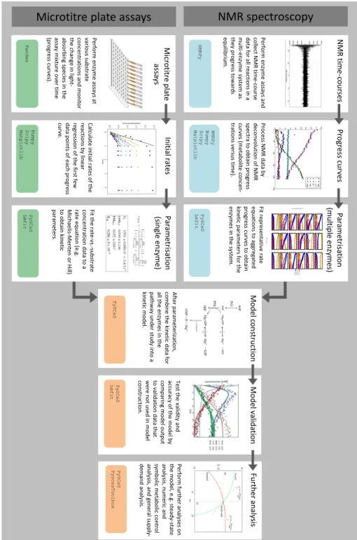
The main workflow for bottom-up kinetic model construction in systems biology, as described
in this paper, is summarised in Figure1. Enzyme-kinetic data were obtained in one of two ways:
either, progress curves for a reaction or group of reactions were acquired with NMR spectroscopy, which were then parametrised by fitting to a system of ODEs with the appropriate enzyme kinetic rate equations; or alternatively, initial-rate kinetics were performed on a single enzyme, typically with a spectrophotometric assay using microtitre plates, and fitted to a rate equation. In this paper,
one example of each approach is discussed in detail (Sections3.2–3.4); in general, it needs to be repeated
until all of the enzymes in the pathway under study have been characterised.
In the next step, all the kinetic rate equations and parameters were assembled into a model of the complete pathway, which was then validated by comparing its output to experimental data that
were not used for model construction (Section3.5). The workflow subsequently allowed a number of
additional computational analyses to be easily performed on a properly constructed and validated
model (Figure1).
Each of the above steps is described in greater detail in the following sections, emphasising the role of the Python language in ‘gluing’ the various analyses together. The Python modules that were
Per fo rm e n zyme as says an d co lle ct N MR ti me -c o u rs e d ata fo r all re ac ti o n s in a mu lti -e n zyme s ys te m as th ey p ro gre ss to w ard s eq u ilib ri u m. N M R time -c ou rses NMRPy
NMR spectroscopy
Microtitre plate assays
Pro ce ss N MR dat a b y d ec o n vo lu ti o n o f N MR sp ec tr a to o b tai n p ro gre ss cu rve s ( me tab o lite c o n ce n -tr ati o n s ve rs u s ti me ). Pr ogr ess cu rv es NMRPy Numpy Scipy Matplotlib Pe rfo rm e n zyme as says at vari o u s s u b str ate co n ce n tr ati o n s an d mo n ito r th e c h an ge in lig h t-ab so rb in g s p ec ie s i n th e as say mix tu re o ve r ti me (p ro gre ss c u rve s). M ic rot it re p la te assa ys Pandas Fit re p re se n tati ve rat e eq u ati o n s to ag gre gate d p ro gre ss c u rve s to o b tai n ki n eti c p arame te rs fo r th e en zyme s i n th e s ys te m. P ar ame trisa tion (mu lt ip le en zymes) PySCeS Lmfit A fte r p arame te ri zati o n , co mb in e th e ki n eti c d ata fo r all th e e n zyme s in th e p ath w ay u n d er stu d y in to a ki n eti c mo d el. M od el con st ru ct ion PySCeS Fu rt h er an aly sis Per fo rm fu rt h er an alys es o n th e mo d el, e .g . st ead y-state an al ys is, n u me ric an d symb o lic me tab o lic c o n tr o l an alys is , an d g en eral s u p p ly -d eman d an alys is . PySCeS PyscesToolbox Te st th e vali d ity an d ac cu racy o f th e mo d el b y co mp ari n g mo d el o u tp u t to vali d ati o n d ata th at w er e n o t u se d in mo d el co n str u cti o n . M od el valid at ion PySCeS Lmfit Fit th e rate -vs .-s u b str ate co n ce n tr ati o n d ata to a rat e e q u ati o n (e .g . Mi ch ae lis -Me n te n o r H ill) to o b tai n ki n eti c p arame te rs . Par ame trisa tion (single en zy me) PySCeS Lmfit Calcu late in iti al rat es o f th e re ac ti o n s b y lin ear re gre ss io n o f th e fir st few d ata p o in ts o f each p ro gre ss cu rve . In it ial ra tes Numpy Scipy Matplotlib
Figure 1.The basic workflow for integrating enzyme kinetics for systems biology with computational modelling using Python. For a detailed description see main text.
3.2. Enzyme Kinetics from NMR Spectroscopy
Our custom open-source NMR processing Python module, NMRPy [20], facilitated the
bulk-processing and quantification of arrayed NMR spectra that are typically produced by NMR
spectroscopy experiments. Figure2provides the raw NMR spectra and quantification of a representative
experiment on the PGM–ENO reaction couple, where the reaction was initiated by incubating the
lysate with phosphoenolpyruvate. The Supplementary Materials contains aJupyternotebook with
code and annotations to read and process the NMR data for Figure2. To fit the kinetic parameters for
both enzymes, a number of such experiments had to be performed with different initial concentrations
PPM (161.89 MHz)1 0 1 2 3 min. 0 20 40 60 80 100 120 140
(a)
0 20 40 60 80 100 120 140 160 Time (min) 0.0 2.5 5.0 7.5 10.0 12.5 15.0 17.5 20.0 Concentration (mM) 3PG 2PG phosphate TEP PEP(b)
Figure 2. (a) Array of31P-NMR spectra from an incubation ofSaccharomyces cerevisiaelysate with phosphoenolpyruvate. Spectra were acquired 2.6 min apart (repetition time) and processed with NMRPy(apodisation, Fourier transform, phase correction and integration by deconvolution). The peak identities are, from left to right: 3-phosphoglycerate (3PG), 2-phosphoglycerate (2PG), phosphate, triethyl phosphate (TEP, internal standard), and phosphoenolpyruvate (PEP). Original spectra are shown as black lines and the deconvoluted peak areas are shown with filled red colour. (b) Quantification of the spectra after processing withNMRPy. The output from the analysis was concentration-versus-time data. NMRPycan read raw data from the major Nuclear Magnetic Resonance (NMR) instrument vendors and has built-in functions to display both the arrayed spectra and quantified data. Data and annotated code (Jupyternotebook) are provided in the Supplementary Materials.
3.3. Enzyme Kinetics from Spectrophotometric Assays
The Supplementary Materials section contains an annotated Jupyter notebook to illustrate
the processing of kinetic data acquired with a microtitre plate reader. By way of example,
glucose-6-phosphate dehydrogenase was characterised in lysates ofZymomonas mobilisusing initial-rate
kinetics with NAD+as the varying substrate. The absorbance of NADH produced in the reaction was
determined spectrophotometrically at 340 nm. The following steps were involved in the data processing:
Importing data New dataframes were created inpandasfrom a variety of input formats, including
Excel and CSV. Several preprocessing and customisation methods were used (e.g., for the
conversion of date/time fields into a format that can be used by Python), as near-perfect
tabulated data are rarely produced by the associated software and the formats differ between
instrument vendors.
Linear regression The absorbance-versus-time data were subject to linear regression over a suitable time
range to calculate initial rates. The attachedJupyternotebook provides two tools (using interactive
matplotlibgraphs, and usingipywidgets), which were used to efficiently apply this analysis to a large number of datasets.
Preprocessing data Thepandaslibrary provided functions to easily normalise the data, either to
a single entry, a single row, or an entire dataframe. Further, Python functions were written to automate repetitive processing tasks in a consistent way. Examples of such normalisations included subtraction of blank readings, the conversion of absorbance values to concentrations, or the subtraction of the initial time reading from subsequent time data.
Fitting data For fitting of initial rate data to an enzyme-kinetic rate equation (e.g., the Michaelis–Menten
equation), the Python packagelmfit[24] provided a high-level interface to various non-linear
optimization and curve fitting routines with access to both global and local optimisation
algorithms. This is further discussed in Section3.4below.
Data Visualization A leading visualisation and 2D-plotting library for Python ismatplotlib, which was
andscipy, and its excellent integration intoJupyternotebooks. Figure3shows the experimental data and model fit (see below) for this experiment.
0
1
2
3
4
5
6
[NAD
+] (mM)
0.0
0.2
0.4
0.6
0.8
1.0
v (
m
ol/
m
in/
m
g
pr
ot
ein
)
Figure 3. Kinetic characterisation of glucose-6-phosphate dehydrogenase in lysates ofZ. mobilisby initial rate kinetics. Lysates were incubated with a fixed concentration of glucose-6-phosphate and varying concentrations of NAD+. The graph shows initial rate data for varying NAD+concentrations (points, mean±SE of triplicate determinations) and the kinetic equation fit (line). Further details and code are available in the supplementaryJupyternotebook.
3.4. Fitting Experimental Data to Obtain Kinetic Parameters
Figure3shows a fit of the Michaelis–Menten equation to experimental data for the enzyme
glucose-6-phosphate dehydrogenase as a function of varying NAD+concentrations (see Section3.3).
Non-linear regression of the rate-versus-concentration data using the Pythonlmfitmodule yielded
the following kinetic parameters: Vmax= 1.15±0.02µmol/min/mg protein,KM = 0.27±0.02 mM.
Further details and fitting code are provided in theJupyternotebook in the Supplementary Materials.
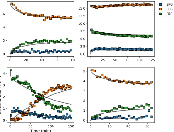
To obtain kinetic parameters from NMR time-courses of multi-enzyme systems, the experimental
concentration-versus-time data were fitted to a kinetic ODE model of the reaction system. Figure4
shows a representative example of four progress curves for the PGM–ENO couple at different initial
concentrations of substrates and products, where the arrayed NMR spectra have already been processed
to calculate concentration time-courses (see Section3.2). Note that some of the reactions ran in reverse
and in one case more than one metabolite was present at the start of the assay. The lines represent the PySCeSmodel output after fitting with the Pythonlmfitmodule, with the parameters fitted toallof the datasets, not only those shown here.
The Supplementary Materials contains all the datasets (not only the representative ones shown
here) as well as aJupyternotebook with the annotated fitting code that provided the fitted parameters
0
20
40
60
80
0
2
4
6
0
25
50
75
100
125
0.0
2.5
5.0
7.5
10.0
12.5
15.0
2PG
3PG
PEP
0
50
100
150
Time (min)
0
1
2
3
4
Concentration (mM)
0
20
40
60
0
1
2
3
4
5
Figure 4. Example of experimental and simulated data for the phosphoglycerate mutase–enolase (PGM–ENO) couple studied by NMR in S. cerevisiae lysates incubated with different starting
concentrations of substrates and products. Square symbols represent experimental data and solid lines represent the simulated model data after parameter optimisation to all data sets simultaneously. Abbreviations: 2PG, 2-phosphoglycerate; 3PG, 3-phosphoglycerate; PEP, phosphoenolpyruvate. 3.5. Assembly and Validation of a Larger Kinetic Model of a Pathway
Once all the enzymes of a pathway under study have been characterised as described in
Sections3.2–3.4, the next step was to combine this information into a kinetic model. The process of
bottom-up model construction has been reviewed [7] and will not be repeated in detail here, other than
to emphasise the importance of a set of consistent enzyme data, especially in regard to the enzyme activities and kinetics, which should all have been determined under the same in vivo-like conditions
(e.g., [25,26]).
Subsequently, the role of the model validation step was to test the accuracy of the predictions of
the model. By investigating how well the model reproducedindependentexperimental data that were
not usedin the model construction process itself (i.e., for fitting the model parameters), this allowed us to assess the quality of the model.
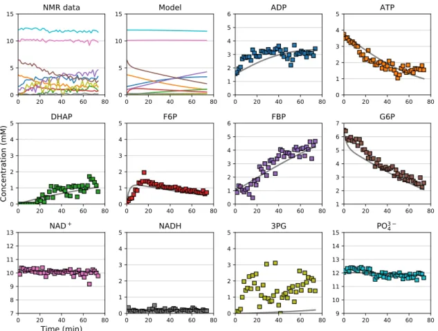
By way of example, Figure5shows the output from a kinetic model ofE. coliglycolysis plotted
together with independent metabolite time-courses determined in situ usingE. colicells permeabilised
with detergent. The Supplementary Materials contains aJupyternotebook with code, model description
and data to recreate Figure5.
While there were some discrepancies between the data and the model fit, the general agreement was remarkable considering that these are independent validation data. The discrepancies, as well as further possible analyses, are considered in the Discussion.
0 20 40 60 80 0 5 10 15
NMR data
0 20 40 60 80 0 5 10 15Model
0 20 40 60 80 0 1 2 3 4 5 6ADP
0 20 40 60 80 0 1 2 3 4 5ATP
0 20 40 60 80 0 1 2 3 4 5Concentration (mM)
DHAP
0 20 40 60 80 0 1 2 3 4 5F6P
0 20 40 60 80 0 1 2 3 4 5 6FBP
0 20 40 60 80 1 2 3 4 5 6 7G6P
0 20 40 60 80Time (min)
7 8 9 10 11 12 13NAD
+ 0 20 40 60 80 0 1 2 3 4 5NADH
0 20 40 60 80 0 1 2 3 4 53PG
0 20 40 60 80 9 10 11 12 13 14 15PO
34Figure 5.Validation of a kinetic model by comparison to independent experimental data. The data points are quantified NMR time-courses from an in situ experiment with permeabilisedE. colicells, starting out with 7 mM G6P, 4 mM ATP, 2 mM ADP, 12 mM phosphate, and 10 mM NAD+. The lines are simulation output from a kinetic model ofE. coliglycolysis, assembled from kinetic measurements on the individual enzymes as outlined in Sections3.2–3.4. Adapted from [20]. Non-standard abbreviations: DHAP, dihydroxy-acetone phosphate; F6P, fructose-6-phosphate; FBP, fructose-1,6-bisphosphate; G6P, glucose-6-phosphate; 3PG, 3-phosphoglycerate.
3.6. Further Model Analysis: MCA, GSDA and PyscesToolbox
Once a kinetic model for a pathway has been constructed and properly validated, it can be subject to a variety of analyses to gain further insight into its regulatory function. A fundamental example
is metabolic control analysis (MCA) [27,28], which aims to quantify the contribution of each of the
steps in a pathway to the control of flux or metabolite concentrations, and thus to identify key control
points. PySCeShas built-in functions to perform MCA directly. Other analyses, based on MCA,
include supply-demand analysis (SDA) [29,30] and its generalised variant GSDA [31], symbolic MCA
(SymCA) [32,33], as well as a framework,ThermoKin, that dissects the contributions of thermodynamic
and kinetic aspects to enzyme regulation [34].
The above-mentioned analysis frameworks have been incorporated into a Python module,
PySCeSToolbox[35], which uses theJupyternotebook andIPythonkernel to analyse the models
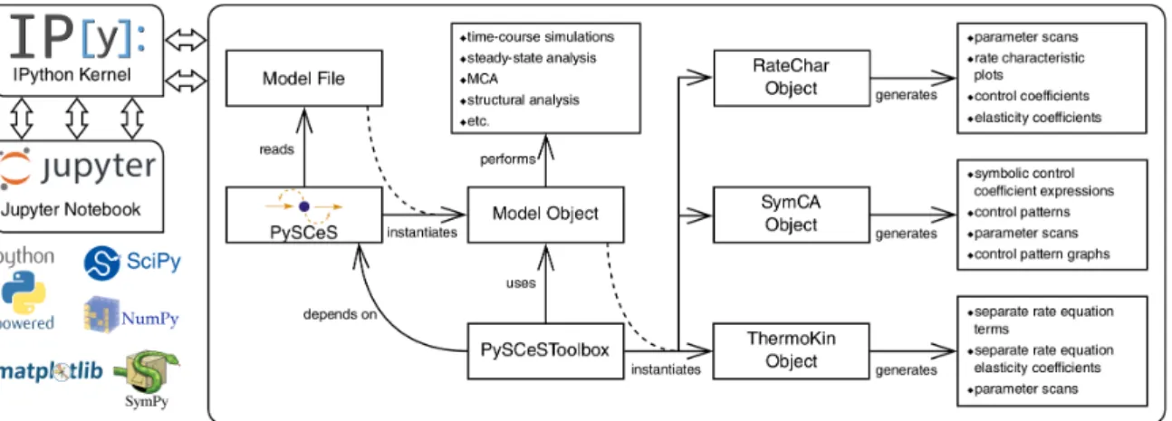
withPySCeSand visualise the output in various interactive ways. Figure6summarises the overall
architecture and workflow ofPySCeSToolbox. At the centre of the analysis is aPySCeSmodel object
which can be used to instantiate one of three analysis objects:
RateChar This module performs GSDA by fixing each variable metabolite in turn (thus making it a system parameter) and varying it below and above its steady-state value. This allows one to identify regulatory metabolites as well as routes of regulation in the network. This approach
was computationally applied [36] to the analysis of published models of pyruvate metabolism in Lactococcus lactis[37] and aspartate-derived amino acid synthesis inArabidopsis thaliana[38]. SymCA This module performs symbolic metabolic control analysis by generating algebraic expressions
for the control coefficients in terms of the elasticity coefficients, using theSymPyPython module
for symbolic algebra [39]. These expressions are then used to evaluate and visualise so-called
control patterns in the network and quantify their relative contribution to the overall value of the
control coefficient. A control coefficient can thus be dissected into its most important components.
ThermoKin This module calculates, for each reversible reaction in the model, the contribution of thermodynamics and kinetics to the enzyme regulation at a particular steady state using the
formalism described in [34]. This contribution may vary as conditions change (e.g., as a result
of changes in some model parameters), as the reaction operates closer to or further away from equilibrium.
SymCAandThermoKinwere applied [40] to the above-mentioned model of pyruvate metabolism [37]. The main point of this section is to illustrate that fine-grained model analysis can be performed within
the same computational framework as the model construction and validation, using Python andJupyter
notebooks; there is no need to change to a new system. The paper describingPySCeSToolbox[35] has
example notebooks as supplementary information, illustrating each of the three module functionalities;
these will not be repeated here. The detailed model analyses in [36,40] are also accompanied byJupyter
notebooks, allowing readers to reproduce the findings.
Figure 6. PySCeSToolboxarchitecture and workflow. PySCeSinstantiates a model object from file, which is then used byPySCeSToolboxto instantiate an analysis tool object. The recommended usage involves running these processes within an IPythonkernel with which the user interacts via theJupyternotebook. The bottom-left corner shows some of the main technologies used by PySCeSToolbox. Refer to [35] for details. Reproduced with permission from Christensen et al., Bioinformatics; published by Oxford University Press, 2018.
4. Discussion
In this paper we have presented a workflow for experimental and computational systems biology that harnesses the powerful capabilities of the Python programming language in terms of both
computation and data visualisation and makes extensive use of theIPythonenvironment andJupyter
notebooks as an interactive platform. The workflow involves processing of raw enzyme-kinetic data, obtained either from microtitre plate assays or from arrayed NMR spectra, to obtain initial rates or progress curves, respectively. These data are then fitted to kinetic equations to obtain enzyme-kinetic parameters, which are used to construct a kinetic model of the pathway. The model is validated by comparison to independent experimental data, and can be further analysed to identify control points or regulatory metabolites. The workflow allows for easy-to-follow data processing, from the original NMR or plate reader data to the final fitted parameter values and kinetic model output.
One compelling aspect of this workflow is the ability to pass information from one Python software to another to create a versatile computational pipeline. For example, microtitre plate readers
typically produce tabulated time-versus-absorbance data, which can be in several formats (CSV, Excel,
plain text, etc.). Python has useful modules for dealing with each of these; the data analysis library pandas[15] (https://pandas.pydata.org) is specifically suited to this task, allowing the data to be
restructured into anumpyarray orpandasdata frame, analysed by any number ofscipytools, passed
into a computational systems biology software such asPySCeS, and finally visualised using the
matplotlibplotting library. While all of these functionalities are available in standalone software
packages, the ability to perform all the analyses within a single environment provided by theJupyter
notebook using scripts that can be automated, is incredibly powerful.
The workflow described makes extensive use of additional modules and libraries, which are available in the scientific Python ecosystem and simplify repetitive or mundane analysis tasks.
For example, while the system of ODEs describing the reaction system discussed in Figure4could
in principle be coded manually [41], our simulation softwarePySCeS[18] automatically generates
ODEs from an input file containing rate and stoichiometric equations.PySCeSadditionally has the
functionality to output simulations at specified custom time points, which facilitates the fitting of NMR
time-courses to kinetic models with thelmfitmodule [24].
When obtaining kinetic parameters from reaction time-courses using NMR, targeted reaction exclusion within a system by enzyme or cofactor omission is essential. Often, many reactions cannot be measured directly and enzyme-kinetic parameters must be determined by fitting models iteratively to datasets from an incrementally expanding system using parameters from earlier iterations to fit the unknown parameters in the larger system. It is important to limit the size of the system of reactions in this way, as fitting too many reactions (and their associated kinetic parameters) at once may lead to
unidentifiable parameters [42].
One of the challenges often encountered in bottom-up kinetic model construction is a discrepancy
between model and data during the validation process (see, e.g., the 3PG dataset in Figure5). To a certain
extent, this is expected considering that these are independent validation data that werenotused
in the parameter fitting. To further investigate this, additional analyses could be done, e.g., theχ2
(discrepancy between model and data) could be calculated, or another validation dataset could be
plotted and compared to the current one. If different models are available, they can be compared in
terms of how well they fit the data [20,43]. The specific dataset could also be used to further fit and
refine the model, which would improve the agreement between model and data. It is important to note, however, that in this case they are no longer independent validation data, and the model would
have to be validated against additional independent experimental data if these are available [7].
There are compelling reasons for choosing Python as programming language for this workflow. Python is relatively easy to learn compared to other programming languages; the language was designed with a very human-readable format and does not contain the syntactical minutiae of lower
level programming languages [44]. This lowers the barrier of entry and broadens the availability of the
analysis platform [45]. In addition to being able to run on different operating systems, Python can
integrate with other programming languages and execute Fortran or C code at near-native speeds using
the modulesf2py[46], which is part ofnumpy, andcython[47] (https://cython.org). This means that
increased readability and interpreted code do not have to come at the expense of computational power and speed, as Fortran and C code can be readily wrapped to run natively in Python by using “interfaces
to low-level high-performance software in a high-level programming environment” [46]. Furthermore,
the interpreted nature of Python allows scripts to easily be transferred between collaborators without
recompiling, meaning that script can be executed on machines with different architectures to produce
identical results [44]. This greatly facilitates collaborations between groups and simplifies collaborations
within groups.
In addition, the Python programming language and the libraries described in this paper are open-source. The scientific Python community is active and supportive and organises annual SciPy
and EuroSciPy conferences (https://conference.scipy.org/), which facilitates its adoption. This creates a feed-forward mechanism where researchers can work and develop new tools in Python because these can be easily integrated into existing software pipelines. The workflow described in this paper latches on to the above feed-forward mechanism by integrating various tools. As such, the list is by no means exhaustive but rather a collection of examples that we use in day-to-day analyses. We do not claim that Python is the best, nor is the aim of this paper to provide a systematic comparison of programming languages or tools; rather, it is an illustration of an adaptable and expandable workflow that has proven useful in our hands. In addition, while our examples in the Supplementary Materials
are presented asJupyternotebooks, this is not a strict requirement and the analysis could have been
performed with a series of Python scripts. The interactive nature ofJupyter, as well as its capabilities
for annotation, structuring and visualisation, just provided additional functionality.
To further substantiate the case for Python in systems biology, we note that, while we have focussed in this paper on those programs and libraries that are most frequently used in our group, researchers have a wide choice of software, many of which are either written in Python or expose
a Python API (summarised in the SBML software matrix, seehttp://sbml.org/SBML_Software_Guide/
SBML_Software_Matrix). Each of these programs is dedicated to particular analysis tasks, and they
will not all be covered in detail here. To mention only a few:Tellurium[48] is a Python-based integrated
environment for modelling and reproducibility analysis that makes use oflibRoadRunner[49] as
the default simulation engine;modelbase[50] has a focus on kinetic modelling similar toPySCeS;
COBRAPy[51] andCBMPy(http://cbmpy.sourceforge.net/) have a focus on constraint-based modelling
of large stoichiometric networks; ScrumPy[52] can do both, but has a focus on constraint-based
modelling;DMPy[53] is a Python package for the automated construction of mathematical models of
large-scale metabolic systems by searching parameters from online resources and matching measured reaction rates. Importantly, by working in a Python environment, the user has the flexibility to interact with any of these programs as required and to easily expand existing or create new workflows.
In addition, many of the leading computational systems biology software programs (e.g., Copasi [54])
expose a Python API, making it possible to easily interface with these programs from within Python
andPySCeSif needed.
An additional challenge faced by systems biology researchers is the need to share data and
resources, often between different platforms. In this context standards are becoming increasingly
important: SBML [19] facilitates the exchange of models in a standard format across simulation tools.
Curated models are stored in databases such as JWS Online [55] and BioModels [56], facilitating their
distribution and increasing their availability. The FAIRDOM project [57] aims to develop frameworks
and guidelines to make data more Findable, Accessible, Interoperable and Reusable. This project
has produced the FAIRDOMHub which uses the SEEK [58] open-source web platform with tools for
collating and annotating datasets, models, simulations and research outcomes. SEEK has a JavaScript Object Notation (JSON) API for uploading and downloading files, and Python supports JSON natively, facilitating integration into Python workflows. A natural extension of the workflow presented here would thus be the development of a SEEK interface.
5. Conclusions
We have demonstrated how the Python programming language can act as a glue to interface
between different analysis tools required for the construction, validation and analysis of kinetic models
in bottom-up systems biology. Our workflow enables investigators to focus on the scientific problem
instead of issues of data integration between platforms. TheJupyternotebook is an ideal e-labbook
and allows the user to keep everything related to a particular analysis in one place, including raw data, graphical output and descriptive annotations.
Supplementary Materials: The following are available at http://www.mdpi.com/2227-9717/7/7/460/s1, Document S1: PDF with instructions for running supplementary notebooks; Archive S2: ZIP archive with supplementary notebooks and associated data files.
Author Contributions: Conceptualization, J.M.R.; methodology, C.J.S, C.T.v.S., J.W., J.M.R.; software, C.J.S., C.T.v.S., J.W., J.M.R.; validation, M.B., C.J.B.; formal analysis, C.J.S, C.T.v.S., J.W.; investigation, C.J.S, C.T.v.S., J.W.; resources, J.M.R.; data curation, M.B., C.J.B.; writing—original draft preparation, all authors; writing—review and editing, J.M.R., C.J.B.; visualization, M.B., C.J.S., J.W., J.M.R.; supervision, J.M.R.; project administration, J.M.R.; funding acquisition, J.M.R.
Funding:This research was funded by the National Research Foundation (South Africa), grant numbers 93466, 93670, and 114748, as well as by Stellenbosch University (student scholarships to C.J.S. and M.B.). The APC was funded in part from the Open Access Publication Fund of Stellenbosch University.
Conflicts of Interest: The authors declare no conflict of interest. The funders had no role in the design of the study; in the collection, analyses, or interpretation of data; in the writing of the manuscript, or in the decision to publish the results.
Abbreviations
The following abbreviations are used in this manuscript: API Application Programming Interface
ENO Enolase
FID Free Induction Decay
GSDA Generalised Supply-Demand Analysis JSON JavaScript Object Notation
MCA Metabolic Control Analysis NMR Nuclear Magnetic Resonance ODE Ordinary Differential Equation OSI Open Source Initiative PGM Phosphoglycerate Mutase
SBML Systems Biology Markup Language SDA Supply-Demand Analysis
References
1. Kitano, H. International alliances for quantitative modeling in systems biology. Mol. Syst. Biol. 2005,
1, 2005.0007. [CrossRef] [PubMed]
2. Westerhoff, H.V.; Alberghina, L. Systems Biology: Did we know it all along? InSystems Biology; Alberghina, L., Westerhoff, H.V., Eds.; Springer: Berlin, Germany, 2005; pp. 3–9. [CrossRef]
3. Snoep, J.L.; Bruggeman, F.; Olivier, B.G.; Westerhoff, H.V. Towards building the silicon cell: A modular approach. Biosystems2006,83, 207–216. [CrossRef] [PubMed]
4. Bruggeman, F.J.; Westerhoff, H.V. The nature of systems biology. Trends Microbiol.2007,15, 45–50. [CrossRef] [PubMed]
5. Rohwer, J.M.; Hanekom, A.J.; Crous, C.; Snoep, J.L.; Hofmeyr, J.H.S. Evaluation of a simplified generic bi-substrate rate equation for computational systems biology. IEE Proc. Syst. Biol. 2006,153, 338–341. [CrossRef]
6. Rohwer, J.M.; Hanekom, A.J.; Hofmeyr, J.H.S. A universal rate equation for systems biology. Experimental Standard Conditions of Enzyme Characterizations. InProceedings of the 2nd International Beilstein Workshop; Hicks, M.G., Kettner, C., Eds.; Beilstein-Institut zur Förderung der Chemischen Wissenschaften: Frankfurt, Germany, 2007; pp. 175–187.
7. Rohwer, J.M. Kinetic modelling of plant metabolic pathways. J. Exp. Bot.2012,63, 2275–2292. [CrossRef] 8. Ingalls, B. Mathematical Modelling in Systems Biology: An Introduction; MIT Press: Cambridge, MA, USA,
2012; p. 386.
9. Jaqaman, K.; Danuser, G. Linking data to models: Data regression. Nat. Rev. Mol. Cell Biol.2006,7, 813–819. [CrossRef]
10. John, R.A. Photometric assays. InEnzyme Assays. A Practical Approach, 2nd ed.; Eisenthal, R., Danson, M.J., Eds.; Oxford University Press: Oxford, UK, 2002; Chapter 2, pp. 49–78.
11. Welling, G.W.; Scheffer, A.J.; Welling-Wester, S. Determination of enzyme activity by high-performance liquid chromatography. J. Chromatogr. B1994,659, 209–225. [CrossRef]
12. Eicher, J.J.; Snoep, J.L.; Rohwer, J.M. Determining enzyme kinetics for systems biology with Nuclear Magnetic Resonance spectroscopy. Metabolites2012,2, 818–843. [CrossRef]
13. Van der Walt, S.; Colbert, S.C.; Varoquaux, G. The NumPy array: A structure for efficient numerical computation. Comput. Sci. Eng.2011,13, 22–30. [CrossRef]
14. Jones, E.; Oliphant, T.; Peterson, P. SciPy: Open Source Scientific Tools for Python. 2001. Available online: http://www.scipy.org/(accessed on 12 July 2019).
15. McKinney, W. Data Structures for Statistical Computing in Python. In Proceedings of the 9th Python in Science Conference, Austin, TX, USA, 28 June–3 July 2010; pp. 51–56.
16. Hunter, J.D. Matplotlib: A 2D graphics environment. Comput. Sci. Eng.2007,9, 90–95. [CrossRef]
17. Anaconda Software Distribution. Version 2-2.4.0. Computer Software. 2017. Available online: https:
//www.anaconda.com(accessed on 12 July 2019).
18. Olivier, B.G.; Rohwer, J.M.; Hofmeyr, J.H.S. Modelling cellular systems with PySCeS.Bioinformatics2005,
21, 560–561. [CrossRef] [PubMed]
19. Hucka, M.; Finney, A.; Sauro, H.M.; Bolouri, H.; Doyle, J.C.; Kitano, H.; Arkin, A.P.; Bornstein, B.J.; Bray, D.; Cornish-Bowden, A.; et al. The systems biology markup language (SBML): A medium for representation and exchange of biochemical network models. Bioinformatics2003,19, 524–531. [CrossRef] [PubMed] 20. Eicher, J.J. Understanding Glycolysis inEscherichia coli: A Systems Approach using Nuclear Magnetic
Resonance Spectroscopy. Ph.D. Thesis, Stellenbosch University, Stellenbosch, South Africa, 2013.
21. Pérez, F.; Granger, B.E. IPython: A system for interactive scientific computing. Comput. Sci. Eng. 2007,
9, 21–29. [CrossRef]
22. Kluyver, T.; Ragan-Kelley, B.; Pérez, F.; Granger, B.E.; Bussonnier, M.; Frederic, J.; Kelley, K.; Hamrick, J.B.; Grout, J.; Corlay, S.; et al. Jupyter Notebooks—A publishing format for reproducible computational workflows. InPositioning and Power in Academic Publishing: Players, Agents and Agendas, Proceedings of the 20th International Conference on Electronic Publishing, Göttingen, Germany, June 2016; Loizides, F., Schmidt, B., Eds.; IOS Press: Amsterdam, The Netherlands, 2016; pp. 87–90. [CrossRef]
23. Swanepoel, C.J. A systematic Investigation into the Quantitative Effect of pH Changes on the Upper Glycolytic Enzymes ofEscherichia coliandSaccharomyces cerevisiae. Master’s Thesis, Stellenbosch University, Stellenbosch, South Africa, 2018.
24. Newville, M.; Stensitzki, T.; Allen, D.B.; Ingargiola, A. LMFIT: Non-linear least-square minimization and curve-fitting for Python. Zenodo2014. [CrossRef]
25. Van Eunen, K.; Bouwman, J.; Daran-Lapujade, P.; Postmus, J.; Canelas, A.B.; Mensonides, F.I.C.; Orij, R.; Tuzun, I.; van den Brink, J.; Smits, G.J.; et al. Measuring enzyme activities under standardized in vivo-like conditions for systems biology. FEBS J.2010,277, 749–760. [CrossRef]
26. García-Contreras, R.; Vos, P.; Westerhoff, H.V.; Boogerd, F.C. Why in vivo may not equal in vitro—New effectors revealed by measurement of enzymatic activities under the same in vivo-like assay conditions.
FEBS J.2012,279, 4145–4159. [CrossRef] [PubMed]
27. Kacser, H.; Burns, J.A. The control of flux. Symp. Soc. Exp. Biol.1973,27, 65–104. [CrossRef] [PubMed] 28. Heinrich, R.; Rapoport, T.A. A linear steady-state treatment of enzymatic chains. General properties,
control and effector strength. Eur. J. Biochem.1974,42, 89–95. [CrossRef]
29. Hofmeyr, J.H.S.; Cornish-Bowden, A. Regulating the cellular economy of supply and demand. FEBS Lett.
2000,476, 47–51. [CrossRef]
30. Hofmeyr, J.H.S.; Rohwer, J.M. Supply-demand analysis: A framework for exploring the regulatory design of metabolism. Methods Enzymol.2011,500, 533–554. [CrossRef]
31. Rohwer, J.M.; Hofmeyr, J.H.S. Identifying and characterising regulatory metabolites with generalised supply-demand analysis. J. Theor. Biol.2008,252, 546–554. [CrossRef]
32. Reder, C. Metabolic control theory: A structural approach. J. Theor. Biol.1988,135, 175–201. [CrossRef] 33. Hofmeyr, J.H.S. Metabolic control analysis in a nutshell. In Proceedings of the 2nd International Conference
on Systems Biology, Pasadena, CA, USA, 5–7 November 2001; Yi, T.M., Hucka, M., Morohashi, M., Kitano, H., Eds.; Omnipress: Madison, WI, USA, 2001; pp. 291–300.
34. Rohwer, J.M.; Hofmeyr, J.H.S. Kinetic and thermodynamic aspects of enzyme control and regulation. J. Phys. Chem. B2010,114, 16280–16289. [CrossRef] [PubMed]
35. Christensen, C.D.; Hofmeyr, J.H.S.; Rohwer, J.M. PySCeSToolbox: A collection of metabolic pathway analysis tools. Bioinformatics2018,34, 124–12. [CrossRef] [PubMed]
36. Christensen, C.D.; Hofmeyr, J.H.S.; Rohwer, J.M. Tracing regulatory routes in metabolism using generalised supply-demand analysis. BMC Syst. Biol.2015,9, 89. [CrossRef] [PubMed]
37. Hoefnagel, M.H.N.; Starrenburg, M.J.C.; Martens, D.E.; Hugenholtz, J.; Kleerebezem, M.; Swam, I.I.V.; Bongers, R.; Westerhoff, H.V.; Snoep, J.L. Metabolic engineering of lactic acid bacteria, the combined approach: Kinetic modelling, metabolic control and experimental analysis. Microbiology2002,148, 1003–1013. [CrossRef] [PubMed]
38. Curien, G.; Bastien, O.; Robert-Genthon, M.; Cornish-Bowden, A.; Cárdenas, M.L.; Dumas, R. Understanding the regulation of aspartate metabolism using a model based on measured kinetic parameters.
Mol. Syst. Biol.2009,5, 271. [CrossRef]
39. Meurer, A.; Smith, C.P.; Paprocki, M.; ˇCertík, O.; Kirpichev, S.B.; Rocklin, M.; Kumar, A.; Ivanov, S.; Moore, J.K.; Singh, S.; et al. SymPy: Symbolic computing in Python. PeerJ Comput. Sci.2017,3, e103. [CrossRef] 40. Christensen, C.D.; Hofmeyr, J.H.S.; Rohwer, J.M. Delving deeper: Relating the behaviour of a metabolic
system to the properties of its components using symbolic metabolic control analysis. PLoS ONE2018,
13, e0207983. [CrossRef]
41. Olivier, B.G.; Rohwer, J.M.; Hofmeyr, J.H.S. Modelling cellular processes with Python and SciPy.
Mol. Biol. Rep.2002,29, 249–254. [CrossRef]
42. Ashyraliyev, M.; Fomekong-Nanfack, Y.; Kaandorp, J.A.; Blom, J.G. Systems biology: Parameter estimation for biochemical models. FEBS J.2009,276, 886–902. [CrossRef] [PubMed]
43. Cedersund, G.; Roll, J. Systems biology: Model based evaluation and comparison of potential explanations for given biological data. FEBS J.2009,276, 903–922. [CrossRef] [PubMed]
44. Ekmekci, B.; Mcanany, C.E.; Mura, C. An Introduction to Programming for Bioscientists: A Python-Based Primer. PLoS Comput. Biol.2016,12, e1004867. [CrossRef] [PubMed]
45. Hinsen, K. High-level scientific programming with Python. In Proceedings of the International Conference on Computational Science—Part III, Amsterdam, The Netherlands, 21–24 April 2002; Sloot, P.M., Tan, C.J.K., Dongarra, J., Hoekstra, A.G., Eds.; Springer: Berlin/Heidelberg, Germany, 2002; pp. 691–700.
46. Peterson, P. F2PY: A tool for connecting Fortran and Python programs. Int. J. Comput. Sci. Eng.2009,4, 296. [CrossRef]
47. Dalcin, L.; Bradshaw, R.; Smith, K.; Citro, C.; Behnel, S.; Seljebotn, D. Cython: The best of both worlds.
Comput. Sci. Eng.2011,13, 31–39. [CrossRef]
48. Choi, K.; Medley, J.K.; Cannistra, C.; König, M.; Smith, L.; Stocking, K.; Sauro, H.M. Tellurium: A Python based modeling and reproducibility platform for systems biology. bioRxiv2016. Available online:https:
//www.biorxiv.org/content/early/2016/06/02/054601.full.pdf(accessed on 12 July 2019). [CrossRef]
49. Somogyi, E.T.; Bouteiller, J.M.; Glazier, J.A.; König, M.; Medley, J.K.; Swat, M.H.; Sauro, H.M. libRoadRunner: A high performance SBML simulation and analysis library.Bioinformatics2015,31, 3315–3321. [CrossRef] 50. Ebenhöh, O.; van Aalst, M.; Saadat, N.P.; Nies, T.; Matuszy ´nska, A. Building mathematical models of
biological systems with modelbase. J. Open Res. Softw.2018,6. [CrossRef]
51. Ebrahim, A.; Lerman, J.A.; Palsson, B.O.; Hyduke, D.R. COBRApy: COnstraints-Based Reconstruction and Analysis for Python. BMC Syst. Biol.2013,7, 74. [CrossRef]
52. Poolman, M.G. ScrumPy: Metabolic modelling with Python. IEE Proc. Syst. Biol. 2006, 153, 375–378. [CrossRef]
53. Smith, R.W.; van Rosmalen, R.P.; Martins Dos Santos, V.A.P.; Fleck, C. DMPy: A Python package for automated mathematical model construction of large-scale metabolic systems. BMC Syst. Biol.2018,12, 72. [CrossRef] [PubMed]
54. Hoops, S.; Sahle, S.; Gauges, R.; Lee, C.; Pahle, J.; Simus, N.; Singhal, M.; Xu, L.; Mendes, P.; Kummer, U. COPASI—A COmplex PAthway SImulator. Bioinformatics2006,22, 3067–3074. [CrossRef] [PubMed] 55. Olivier, B.G.; Snoep, J.L. Web-based kinetic modelling using JWS Online. Bioinformatics2004,20, 2143–2144.
[CrossRef] [PubMed]
56. Le Novère, N.; Bornstein, B.; Broicher, A.; Courtot, M.; Donizelli, M.; Dharuri, H.; Li, L.; Sauro, H.; Schilstra, M.; Shapiro, B.; et al. BioModels Database: A free, centralized database of curated, published, quantitative kinetic models of biochemical and cellular systems. Nucleic Acids Res. 2006,34, D689–D691. [CrossRef] [PubMed]
57. Wolstencroft, K.; Krebs, O.; Snoep, J.L.; Stanford, N.J.; Bacall, F.; Golebiewski, M.; Kuzyakiv, R.; Nguyen, Q.; Owen, S.; Soiland-Reyes, S.; et al. FAIRDOMHub: A repository and collaboration environment for sharing systems biology research. Nucleic Acids Res.2017,45, D404–D407. [CrossRef]
58. Wolstencroft, K.; Owen, S.; Krebs, O.; Nguyen, Q.; Stanford, N.J.; Golebiewski, M.; Weidemann, A.; Bittkowski, M.; An, L.; Shockley, D.; et al. SEEK: A systems biology data and model management platform.
BMC Syst. Biol.2015,9, 33. [CrossRef] [PubMed] c
2019 by the authors. Licensee MDPI, Basel, Switzerland. This article is an open access article distributed under the terms and conditions of the Creative Commons Attribution (CC BY) license (http://creativecommons.org/licenses/by/4.0/).