IEM Report 39/07 Icosahedral Loudspeaker Array

IEM Report 39/07

Icosahedral Loudspeaker Array

Verfasser:

Franz Zotter

Alois Sontacchi

January 2007

A-8010 Graz, Inffeldgasse 10/3, Tel.:+43/(0)316/389 – 3170, FAX:+43/(0)316/389 – 3171 [email protected] http://iem.at

Herkömmliche Lautsprecherwiedergabe mit einem Lautsprecher kann insbeson-dere den Aspekt der Synthese von Abstrahlungsformen nicht nachbilden. Einzel-lautsprecher haben ihre eigene Abstrahlungswirkung, die in Wirklichkeit sehr weit von der Abstrahlung des reproduzierten Instrumentalklangs abweichen kann. Wir haben, um die Abstrahlungssynthese zu ermöglichen, am Institut für Elektronische Musik und Akustik (IEM) ein ikosaederförmiges Lautsprechersystem gebaut. Dieser Bericht dokumentiert den Aufbau davon, die Bestandteile, sowie erste Messungen und Bewertungen, die an dem neuen Gerät vorgenommen wurden.

Abstract

An aspect that can’t be covered yet by classical loudspeaker playback is radia-tion synthesis. In fact, a single loudspeaker will have its own radiaradia-tion characteris-tics that can be quite different compared to the radiation of the musical instrument it is used to reproduce with. To accomplish this, we have built an icosahedral lous-peaker array system at the Institute of Electronic Music and Acoustics (IEM). This report contains a documentation of its construction, its components, as well as the first measurements and characterizations we have done on this new device.

Contents

1 Introduction 4

2 Design Considerations 4

2.1 Driver Design . . . 4

2.2 Enclosure Size, Lower Cut-Off . . . 4

2.3 Driver Spacing, Upper Cut-Off . . . 5

3 Construction Issues 6 3.1 Preparing and Mounting the Speakers . . . 6

3.2 Cabling and Amplification . . . 7

4 Measurements and Characterization 8 4.1 Measurement Setup . . . 8

4.2 Impulse Response Windowing . . . 9

4.3 MIMO-Description . . . 10

4.4 Exploiting Symmetric Exchange for MIMO-Description . . . 10

4.5 Desired Radiation Pattern . . . 12

4.6 Normalized Steering Error . . . 13

1

Introduction

Our institute has done a lot of research in the domain of multichannel holophonic sound reproduction systems. These, especially Ambisonic, are mainly used to reproduce a soundfield environments in a listening room, or in headphone based playback systems, in order to reproduce the incident sound environment at one listening point (cf. Daniel [1]). In this paper we will consider some kind of inverse application, i.e. the radiation of sound waves from one point with a spherical loudspeaker array (cf. Warusfel et al. [2], Kassakian et al. [3]).

As described by e.g. Daniel [1], Petersen [4], or Li [5], it is necessary to find a suitable set of nodes on a spherical surface for numerical integration. Considering its simplicity in construction, a given limit in the amount of speakers, and its uniform distribution of points, we chose the icosahedron as basic shape for our spherical array.

The acoustical design criterion for the playback system was the fundamental frequency

f0 = 42[Hz] and level of 94dB of the gong ageng we want to synthesize with the

spherical array. Of course, this is a very low frequency, but we also want to inspect radiation characteristics in room acoustic environments at low frequencies.

2

Design Considerations

2.1

Driver Design

Our speaker array shall be capable of reproducing radiation within a range of approx-imately 40[Hz] < f < 4000[Hz]. Therefore, we have chosen a coaxial 61

2["] and 1["]

driver pair with cross over frequency at approximately 2[kHz]1

. We get upper cut-off frequencies for a spherical radiation at k _·rM = 2·π_c·fU = π, i.e. fU1 ≈ 2[kHz],

fU2 ≈13[kHz].

2.2

Enclosure Size, Lower Cut-Off

Measured resonance frequencies of an unmounted speaker without and with mZ =

5g additive mass are (mass difference method, Graber lecture notes [6], Dickason [7], Zwicker [8]):

foS = 59.4[Hz]

foS,Z = 50[Hz].

For the acutal equivalent membrane mass we get (cf. [6], [7], [8])

mg,oS = mZ foS foS,Z 2 −1 . (1)

The membrane stiffness becomes (cf. [6], [7], [8]) Cm,M a= 1 mg,oS·ωoS2 = foS foS,Z 2 −1 mZ·ω2oS . (2)

Finally, with the given membrane radius rM = 6[cm], we are able to calculate the equivalent volume stiffness of the membrane construction (cf. [6], [7], [8]):

Va,M a =ρ·c2·A2M ·Cm,M a=ρ·c2·rm2π· foS foS,Z 2 −1 mZ ·4π2foS2 (3) In numbers, we have Va,M a = 1.2·3402·(6·10−2)2π· 59.4 50 2 −1 5_·10−3_·4π2_59.42 = 0.011[m 3 ] (4)

The volume of an icosahedron is (cf. Ortner [9])

V = 2 3

r

25 +√5_·r3_{, (5)}

for the radiusr= 26.5[cm], we get V = 0.047[m3].

For a box with VB = 0.047[m3], we get the lower cut-off frequency (cf. [6], [7], [8]), assumingfuS ≈foS: fL = 0.93· r 1 + Va,M a VB · fuS = 61[Hz]. (6)

For the closed box, we have a2nd_{order high-pass skirt (cf. [6], [7], [8]). For the frequency}

fGong = 42[Hz] we get the following attenuation:

H(fGong) = −10·log10 " 1 + fL fGong 4# =₋7.4dB. (7)

2.3

Driver Spacing, Upper Cut-Off

We can fit a dodecahedron into our icosahedron to determin the driver spacing. The edges of this dodecahedron connect the centers of the loudspeakers mounted into the icosahedral skeleton. For an icosahedron with (outer) radius r = 33[cm] we get the radius of the insphererin =r

r

· 7+3√5

3·(5+√5) = 26[cm] So the spacing between the speakers

corresponds to the edges of the dodecahedrona = 4·rin

(1+√5)√3 = 19[cm], (cf. Ortner [9]). Using λl 2 = c 2·fu !

= a, we get some upper cut-off frequency for spatial aliasing at

distances smaller thana, so we cannot clearly speak of aliasing for frequencies f > fu. An alternative frequency for aliasing can be given at fu = 3[kHz], selecting a radial direction going through one speaker.

Considering the broadband playback capability of the spherical array system, it is useful to build the speakers into one common enclosure volume. The major drawback, however, is the cross-talk between the speakers over the common enclosure.

3

Construction Issues

3.1

Preparing and Mounting the Speakers

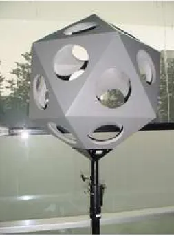
According to the sizes determined above considerations, we have had built an icosahedral skeleton shape out of MDFs (cf. Fig. 1). A loudspeaker stand connector, as well as a multipin connector has been mounted on one of the corners of the icosahedron (see Fig. 4).

Figure 1: The icosahedral skeleton for the loudspeaker array in February 2006.

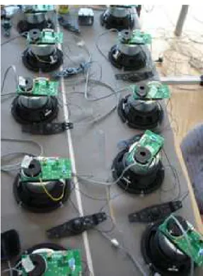
Between March and May 2006, we have connected the cross-over circuits of the coaxially mounted drivers and glued them on the bass speakers (see Fig. 2).

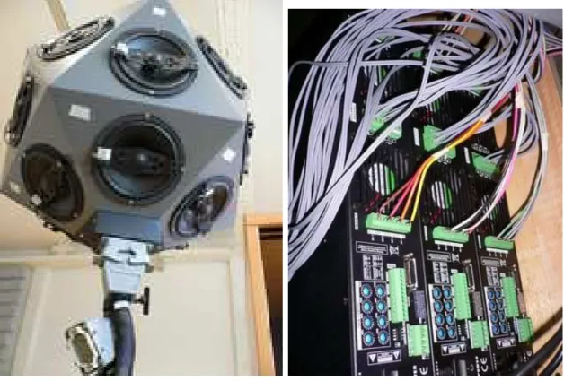
In May 2006, the speakers have been mounted into the enclosure (see Fig. 3). We filled the enclosure loosly with acoustic damping wool.

Figure 2: Joining the cross-over circuits with the speaker drivers in April 2006.

Figure 3: Mounting the speakers in June 2006.

3.2

Cabling and Amplification

We used a 42-pin Multipin-connector for wiring the drivers with the amplifiers, via 13m of 20 ordinary2.5mm2 _{loudspeaker cables. On the other side of the cable, three 8x100W}

multichannel amplifiers are used (cf. Fig. 4). The signals are obtained from a MADI multichannel audio interface and DA-converters for PC. Our PC is running pd

(pure-data) under linux.

Figure 4: Multipin Connectors and amplifier connections.

4

Measurements and Characterization

4.1

Measurement Setup

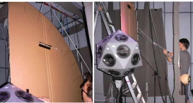
For the first few measurements, we used a circular microphone-array in an acoustically damped room (see Fig. 5).

For a preliminary study, we neglected the non-ideal omnidirectional microphone char-acteristics, and the manufacturing tolerances in the driver properties. Under all these assumptions, we can exploit the icosahedral symmetries. There wer only two mea-surement series using a ten element circular array of 90◦ _{aperture. The speaker array}

was set up in 0◦ _{and 36}◦ _{orientation for the two measurement series consisting of 400}

seperate transfer paths. The 20 measurement points can be expanded to a grid of 172 measurement positions (see Fig. 6). We will explain this a few lines later. We took the measurements using a log-swept sine technique that also delivers some information about nonlinear distortions.

Figure 5: Adjusting the circular array microphones. We disregarded the axial aiming of the microphones.

Figure 6: Virtual measurement grid and actually measured responses (highlighted by the pencil strokes).

4.2

Impulse Response Windowing

Due to size and residual reverberation of the measurement room, we had to use win-dowing techniques to seperate the impulse responses from the room reverberation. An

exponential window starting at 2ms from the direct responses has been applied (see Fig. 7).

Figure 7: We see the impulse responses on a logarithmic scale, normalized to their first peak each in the first picture. In order to suppress the unwanted acoustic reflexions in the measurement chamber, we apply an exponential window. The skirt of the exponential time-domain window starts at4ms using₋11.25dB/[ms] slope; the resulting attenuation can be seen in the picture below.

4.3

MIMO-Description

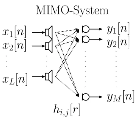
For convenience, we work in the frequency domain at a certain freqency ω. With the (Lx1) input sample vectorX(ω)at the loudspeakers and the (Mx1) output sample vector

Y(ω)at the microphones,

X(ω) = [X1(ω),· · · , XL(ω)]t (8)

Y(ω) = [Y1(ω),· · · , YM(ω)] t

, (9)

we get a (MxL) MIMO-systemH(ω), see also Fig. 8:

H(ω) =    H1,1(ω), · · · , H1,L(ω) ..., _{· · ·} , ... HM,1(ω), · · · , HM,L(ω)   , (10)

according to the equation

Y(ω) =H(ω)_·X(ω). (11)

4.4

Exploiting Symmetric Exchange for MIMO-Description

To obtain the entire rectangularly spaced MIMO transfer function matrix, several column and row interchanging operations are allowed due to the symmetries in the arrangement.

. . . . . . . . . . .

x

[n]

x

[n]

x

[n]

y

[n]

y

[n]

y

[n]

h

[r]

MIMO-System

Figure 8: Measurement setup block diagram.

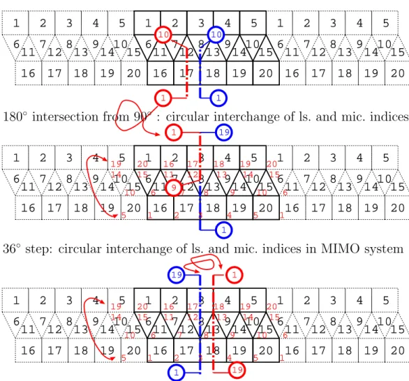
We have measured two cross-sections of the radiated soundfield. All other cross-sections needed (see Fig. 6) can be derived from the two measured by interchanging loudspeaker and microphone indices. A scheme of the icosahedron with numbered surfaces and the microphone cross-sections with microphone numbers is provided in Fig. 9. For the cross-sections at a36◦ _{azimuthally shifted position we have to:}

1. interchange the loudspeaker indices • [1,2,3,4,5]_⇐[20,16,17,18,19]

• [6,7,8,9,10] _⇐[15,11,12,13,14]

• [11,12,13,14,15]_⇐[6,7,8,9,10]

• [16,17,18,19,20]_⇐[1,2,3,4,5]

2. and invert the microphone order

• [1,2, . . . ,19]_⇐[19,18, . . . ,1], according to the scheme drawn in Fig. 9.

Furthermore, due to the symmetries w.r.t the measurement plane, some responses should be equal, i.e. their loudspeaker indices are interchangeable:

• [1,2,3,4,5]_⇔[5,4,3,2,1]

• [6,7,8,9,10]_⇔[10,9,8,7,6]

• [11,12,13,14,15]_⇔[14,13,12,11,15]

1 2 3 4 5 6 7 8 9 10 11 12 13 14 15 16 17 18 19 20 1 2 3 4 5 6 7 8 9 10 11 12 13 14 15 16 17 18 19 20 1 2 3 4 5 6 7 8 9 10 11 12 13 14 15 16 17 18 19 20 1 2 3 4 5 6 7 8 9 10 11 12 13 14 15 16 17 18 19 20 1 2 3 4 5 6 7 8 9 10 11 12 13 14 15 16 17 18 19 20 1 2 3 4 5 6 7 8 9 10 11 12 13 14 15 16 17 18 19 20 1 2 3 4 5 6 7 8 9 10 11 12 13 14 15 16 17 18 19 20 1 2 3 4 5 6 7 8 9 10 11 12 13 14 15 16 17 18 19 20 1 2 3 4 5 6 7 8 9 10 11 12 13 14 15 16 17 18 19 20 17 18 19 20 19 20 16 12 13 14 15 14 15 11 8 9 10 6 10 6 7 3 4 5 1 5 1 2 10 1 10 1 9 1 19 1 19 1 19 1 17 18 19 20 19 20 16 12 13 14 15 14 15 11 8 9 10 6 10 6 7 3 4 5 1 5 1 2

completion from two preliminary test measurements

(assumption: identical and interchangeable speakers)

36

step: circular interchange of ls. and mic. indices in MIMO system

180

intersection from 90

: circular interchange of ls. and mic. indices

Figure 9: Obtaining the entire MIMO grid from index interchanges due to icosahedral symmetries.

4.5

Desired Radiation Pattern

We want to reproduce arbitrary radiation patterns up to the resolution accomplishable with the icosahedral speaker array. The spherical harmonic functions are an appropriate choice of basis functions. With a given set of K = (N + 1)2 _{spherical harmonics, we}

can synthesize radiation patterns up to an angular bandwidth N. In the case of the icosahedral loudspeaker array, we are limited to ofNico = 3, as the system is determined by(N + 1)2

≤20regularly spaced loudspeakers.

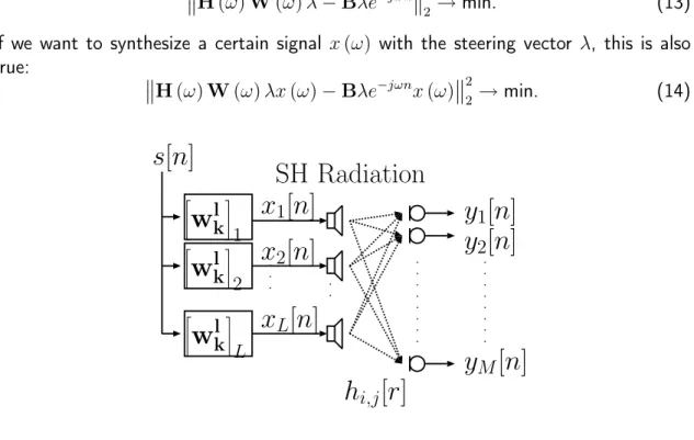
To obtain a specific set ofK target patternsB at the microphone positions (M _×K), we have to invert the MIMO-system. This can be done in frequency domain, using the least squares solution2

, H(ω)W(ω)−Be−jωn 2 2 → min. (12) 2_A† = AHA −1 AH _{is the pseudo-inverse ofA}

W(ω) = H†(ω)_·B_·e−jω·n_,

wheree−jω·n _{is a time-delay ofn samples to make the system causal, and W(ω) is the}

(L_×K) set of complex driving weights for the loudspeakers at the frequency ω. Now, if a target pattern Y can be decomposed into our base set of target patterns

Y=Bλ, the following should hold too:

H(ω)W(ω)λ−Bλe−jωn 2 2 →min. (13)

If we want to synthesize a certain signal x(ω) with the steering vector λ, this is also true: H(ω)W(ω)λx(ω)−Bλe−jωnx(ω) 2 2 →min. (14) . . . . . . . . . . .

x

[n]

x

[n]

x

[n]

y

[n]

y

[n]

y

[n]

h

[r]

w

w

w

s[n]

SH Radiation

Figure 10: Driving filter block diagram for one single radiation pattern.

4.6

Normalized Steering Error

We can assess the quality of the arrangement by using the relations Peter Kassakian described in [10]. It is, however, decisive that we have to use quadrature weights before we start. As a pre-condition for the assessment, the basis of target patterns has to be orthonormal BH

B = I. For the spherical harmonics this only holds for a regularly (uniformly) sampled spherical surface, and not for rectangular sampling. Nevertheless, we can approximate orthonormality by using quadrature weightsC. For this reason, we desire the following orthonormality relation:

(CB)HCB=! I. (15)

In our case, the system is underdetermined and could only be solved by approximation. An intuitive approach to solve this equation, is to assign weights to each point, according to its equivalent surface fraction. The angular grid here, is defined by θk = πk_N

θ, with

sphere betweenθi < θ < θj and its fraction of the whole sphere can be given as (cf. [11], p. 162): Ssl = 2πr2[cos (θi)−cos (θj)], (16) Ssl 4r2_π = cos (θi)−cos (θj) 2 . (17)

Dividing by the azimuthal steps and taking the square root, we get the surface fractions of one single node:

ck,l =        r 1−cos“ π 2Nθ ” 2 , if k = 0, Nθ r cos“ϕk+_2Nθπ ” −cos“ϕk−_2Nθπ ” 2Nϕ , else. (18)

Assigning the quadrature weights to the node points, we get the weighting matrixC=

diag_{c_}. The result(fCB)HfCBof this approximative quadrature is shown in Fig. 11. We have also introduced a scalar normalization factor f that normalizes the diagonal elements to unity: f = v u u ttrace n (CB)HCBo K . (19)

The new weighted least-squares problem considering the quadrature weightsCis:

CH(ω)W(ω)−CBe−jωn 2 2 → min. (20) W(ω) = (CH(ω))†CBe−jωn

Now we are prepared to derive the normalized steering errors of sub-sets Bs of the

spherical harmonics, sharing the same degree k with the dimension (M _× 2k + 1). The procedure can be found in Peter Kassakian’s paper [10]. At first we take the QR

decomposition ofH(ω) (M _×L), with Q2 (M ×M −L): [Q1,Q2] _˜ R 0 =fCH(ω). (21)

The normalized steering error bounds for the subsetBs are determined by the following

singular values: σmin fQ2 H CBs (22) σmax fQ2 H CBs , (23)

where σmin() and σmax() denote the minimum and maximum singular values of the

Figure 11: The quality assessment of our icosahedral speaker, following Peter Kassakian’s paper [10], is quite poor at the moment. Note that the frequency resolution is reduced by windowing to approximately 220[Hz]. Furthermore, we do know yet, how much deviations arise due to our symmetry assumptions.

5

Acknowledgements

We want to thank Josef Schalk the accurate and dignified construction of the MDF skeleton for our icosahedral speaker system. Christian Jochum and Peter Reiner were a

very diligently filling the skeleton with life, i.e. preparing and mounting of the speakers, cabling, helping through the measurerment of the responses. Furthermore, we are grate-ful for the characterization scheme by Peter Kassakian, for the speakers from ITEC-Audio and the financial support from the Zukunftsfonds Steiermark.

References

[1] J. Daniel, Représentation de champs acoustiques, application à la transmission et à la reproduction de scènes sonores complexes dans un contexte multimédia, PhD thesis, Université Paris 6, France, 2000.

[2] O. Warusfel and N. Misdariis, “Sound Source Radiation Synthesis: from Stage Performance to Domestic Rendering,” in116th AES Convention, May 8-11, Berlin, Germany, 2004.

[3] Peter Kassakian, “Magnitude Least-Squares Fitting via Semidefinite Programming with Applications to Beamforming and Multidimensional Filter Design,” in Interna-tional Conference on Acoustics, Speech, and Signal Processing, IEEE, 2005.

[4] Svend Oscar Petersen, Localization of Sound Sources Using 3D Microphone Array, Master’s Thesis, University of Southern Denmark, 2004.

[5] Zhiyun Li, Ramani Duraiswami, and Nail A. Gumerov, “Capture and Recreation of Higher Order 3D Sound Fields Via Reciprocity,” in ICAD2004, 6-9 July, Sidney, Australia, 2004.

[6] Gerhard Graber and Werner Weselak, Elektroakustik, IBK Institut für Breitband-kommunikation, TU-Graz, version 5.0 edition, 2001.

[7] Vance Dickason, Lautsprecherbau, Elektor-Verlag, 1 edition, 2001.

[8] Manfred Zollner and Eberhard Zwicker,Elektroakustik, Springer Verlag, Heidelberg, 3. auflage edition, 1993.

[9] Dieter Ortner, “Die fünf Platonischen Körper,” http://www.zebis.ch/inhalte/unterricht/mathematik/polyeder.pdf, Zen-tralschweizer Bildungsserver, 2003.

[10] Peter Kassakian and David Wessel, “Characterization of Spherical Loudspeaker Arrays,” in 117th _{Convention of the Audion Engineering Society, San Francisco,} 28-31 Oct. 2005.

[11] I.N. Bronstein and K.A. Semandjajew and G. Musiol and H. Mühlig, Taschen-buch der Mathematik, Verlag Harri Deutsch, Thun und Frankfurt am Main, 5. überarbeitete und erweiterte Auflage edition, 2001.