Regional Absorption of Terms of Trade Shocks
E. A. Haddad♣ and F. S. Perobelli♦
Paper prepared for the 41st Congress of the European Regional Science Association
Abstract. As the process of global integration evolves, developing economies become more and more
dependent upon the swings of international markets. Changes in the external environment and economic policy have played a major role in determining the performance of these economies. Terms of trade shocks represent one of the most important issues related to recent developments in low and middle income countries, whose effects have been widely studied in the economic literature. However, attention has always been focused on the national economies, without any consideration of the ability of these economies to absorb these shocks through interregional interactions. In this paper we address this issue using a bottom-up interregional CGE model. It is shown that the degree of integration of the national economies helps to absorb external shocks, decreasing the adverse impacts of negative terms of trade shocks as the economy becomes more integrated.
I. Introduction
As the process of global integration evolves, developing economies become more and more dependent upon the swings of international markets. Whatever country indicators related to the integration with the global economy one considers, the overall trend verified in the last decade points to higher degrees of trade dependence in those countries. For instance, the average share of trade in total GDP has increased from 41.0% to 53.4% in the low and middle income countries in the period 1990-1998, and foreign direct investments in those countries have almost quadrupled in GDP terms, in the same period (WDI, 2000).
The assertion that national economies are increasingly being driven by global rather than local factors is grounded on the recent focus on globalization issues and the implicit assumption that a region’s economic future is inextricably tied with its ability to compete in the international export market. At the national level, attention has also been directed to financial contagion through stock markets.
♣ Department of Economics, University of São Paulo, Brazil
Regional Economics Applications Laboratory, University of Illinois at Urbana-Champaign, USA ehaddad@usp.br
♦
Department of Economics, University of São Paulo, Brazil Department of Economics, Federal University of Juiz de Fora, Brazil
Given the fact that trade becomes a more powerful channel of growth every day, regional analysts place considerable efforts towards the understanding of the role of trade in regional development. Terms of trade shocks receive special attention as these phenomena seem to be very frequent and have significant impacts on the regional economies.
On one hand, internal (active) terms of trade shocks, undertaken by policy makers in the country (region), appear to be a major policy remedy for lower productivity levels in developing countries. Trade liberalization has been widely used as an instrument to the insertion of developing countries in the global economy. The effects of trade reforms, one of the driving forces of the globalization process, have been extensively studied in the international trade literature. On the other hand, these same economies become more and more vulnerable to external (passive) terms of trade shocks. Already in the 1970s, external shocks of commodity booms and oil price hikes had major impacts in developing countries. Macroeconomic adjustment through real exchange rate devaluation was the basic policy recommendation. Institutional constraints, however, preclude many countries to achieve success in their adjustment processes (Devarajan and de Melo, 1987).
More recently, oil price shocks were under the spot again, and the recent trends in commodity prices also brought about concern to major exporters and countries relying heavily on the exports of a few commodities. Attention has usually been focused on the national economies, without any consideration of the ability of these economies to absorb these shocks through interregional interactions. Would more integration at the sub-national level help to absorb negative impacts of terms of trade shocks through substitution effects? Would it depend on the degree of complementarity among regions? In this paper we address this issue using a bottom-up interregional computable general equilibrium model. The remainder of the paper is organized in three sections and an appendix. First, after this introduction, an overview of the CGE model to be used in the simulations is presented, focusing on its general features. Second, the simulation experiment is designed and implemented, and the main results are discussed. Final
remarks follow in an attempt to evaluate our findings and put them into perspective, considering their extension and limitations. An appendix containing the full specification of the CGE model is also presented.
II. The Structure of the Model
The model presented here is an extension of the 1-2-3 model (Devarajan et al., 1997), a simple general equilibrium model designed for determining the relationship between external shocks and policy responses. Following the 1-2-3 tradition, a minimalist model is designed in order to verify how regional interaction at the sub-national level influences the adjustment of external shocks in a national economy under small country assumptions. Agents’ behavior is modeled at the regional level, accommodating variations in the structure of regional economies. The model recognizes the economies of two regions, which are related through trade flows. Results are based on a bottom-up approach – national results are obtained from the aggregation of regional results. The model identifies two producing sectors in each region, and seven commodities: two foreign export goods (sold to foreigners and not demanded domestically), one foreign import good (not produced domestically)1, and two regional goods and two interregional export goods, which are sold within the region and exported to the other region, respectively. The model also identifies a single household in each region, regional governments and one federal government, and a single foreign consumer who trades with each region. Special groups of equations define real flows, nominal flows, prices and equilibrium conditions. There are no primary factors in the model, which underlies the implicit assumption of full employment of the regional fixed endowments.
The schematic structure of the model – without government – presented in Figure 1, shows in a simple interregional open-economy framework the basic decision process of producers and consumers in the model. In each region, the supply relations are generated by considering a two-stage revenue maximization problem of choosing, first, the mix of
1
Although our specification accommodates two region-specific import goods, they are treated as the same good for the sake of explanation.
goods to be exported and sold domestically (CET specification), and, second, the mix of the regional good sold within the region and outside the region (CET). In the demand side, regional household determines the optimal composition of its consumption bundle in a two-stage utility maximization problem (equivalent to maximize total consumption): first, it chooses the composition of domestically produced good and import good (CES specification); second, it decides how much of each regional good to consume (CES). The assumption underlying this two-stage choice relates to the Armington assumption, which considers similar commodities produced in different regions as close substitutes, but unique goods (Armington, 1969).2 Interregional and international trade balances follow from the agents’ decisions. Transportation costs are associated with interregional trade, following Samuelson’s iceberg model, which means that a certain percentage of the transported commodity itself is used up during transportation (Bröcker, 1998). Given the
transport rate ηi, defined as the share of commodity i lost per unit of distance, and the distance between the regions A and B, zAB, the amount arriving in B, if one unit of
output i has been sent from A to B, is exp
(
−ηizAB)
, which is less than unit for positive distances.
2
There is nothing in this conceptual set up that requires these elasticities to be constant, but modellers have tended to use constant elasticity specifications. Hence the use of CET functions for production and CES functions for consumption.
Consumption
Region B
CES DCB MB Production CES CET DPFA = MFB DDB EA DPA CET BR CET DPB DDA DPFB = MFA CET CES Production BWA MA DCA CESThe basic model can be seen as a simple two-stage programming problem.3 Separability of the production and utility functions allows for its solution in a two-stage maximization problem. In the first stage, consumption of the domestic composite good is maximized in each region, subject to technological and interregional balance of trade constraints, and market-clearing condition for the regional goods. The problem is:4
(
2)
2 , , , max , r; r D r r r DD DD DF MF SDC F DD MF r D r r r σ = r= A,B subject to(
r rS r)
r r DPF DD DP G2 , ;θ2 ≤ (1) r r r r r MF PDPF DPF BR PDCMF × − × ≤ 0 ≤∑
r r R B S r D r DD DD ≤In the second stage, consumption of the composite good is maximized in the two regions, subject to technological and international balance of trade constraints.5
(
1)
1 , , ,EmaxDC DP r r r, r; r Mr r r rQ F M DC σ = r = A,B subject to (2)(
r r r)
r r E DP X G1 , ;θ1 ≤ r r r r r M WE E BW WM × − × ≤This programming problem can be depicted graphically. Figure 2 shows the solution for a single region in the special case where international and interregional trade balances are
zero (BWr=0 and BRr =0, ∀r), and transportation costs are negligible (ηi =0).
3
See Devarajan et al. (1997) for the representation of the simpler 1-2-3 model as a programming problem.
4
See the definition of the variables in the appendix.
5
In both cases, the shadow prices of the constraint equations correspond to market prices in the CGE model.
Moreover, it is assumed that world prices are equal to one, so that the slope of the price lines equal one.
Figure 2. Graphical Representation of the Basic Model for a Single Region
II M I BW C PDC/PM DC E PDP/PE P Domestic Market III DP IV II' MF I' BR C' PDD/PDCMF DDD DPF PDD/PDPF P' Regional Market III' DDS IV'
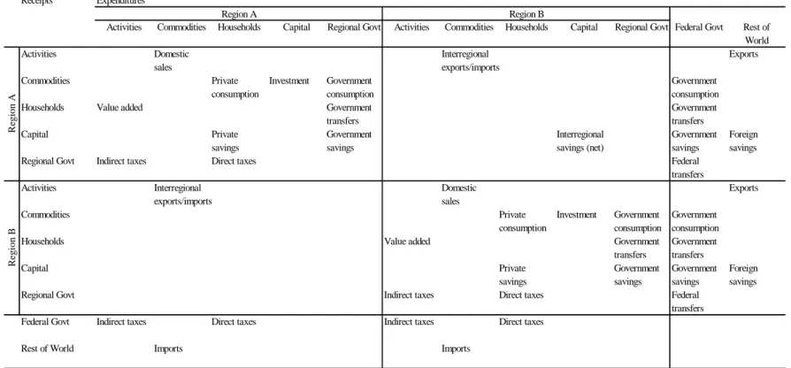
As a starting point for the understanding of the model, the interregional SAM is presented (Figure 3). Nominal flows equations represent macroeconomic balance constraints defined in the SAM (see appendix). The economy is divided into twelve accounts. In each region, goods produced are either sold within the region or exported to the rest of the country and the rest of the world. The production costs include the payments to the production factors – owned by the households in the region – and the payments of taxes to the regional and federal governments. Total supply of goods in a region is given by the domestic production sold domestically, the interregional imports and the purchases abroad. Accordingly, total demand includes private consumption, investment, and government consumption. In addition to the income received in the production process, households receive government transfers, spending their income in the consumption of goods, savings and the payments of direct taxes to the regional and federal governments. Investments in the region are financed by private savings, government savings, net interregional savings and foreign savings, in a typical “four-gap” interregional model.6 Public sector is divided into regional government, which includes the states and the municipalities in the region, and the federal government. In the former case, expenditures are financed by taxes and federal transfers. Federal government deficit arises from tax revenue spent in consumption and transfers in the two regions. Finally, the rest of the world generates foreign savings in the regions through international trade.
Each cell in the SAM, which is a transaction, can be thought of as the outcome of an underlying optimization problem of the relevant institution(s). We can represent the flow in the cell as ) , ; , ( V ξ t tij = p q (3)
where p and q are respectively vectors of relative prices (for goods and factors) and quantities. The vector V is a vector of exogenous factors and ξ is a vector of parameters defining the relevant functional form. The complete specification of the model is provided in the appendix, based on the different groups of equations. The description is organized around four groups of equations: a) real flow equations; b) nominal flow equations; c) equations defining the price system; and d) equilibrium conditions.
6
Figure 3. Schematic Interregional Social Accounting Matrix
Receipts Expenditures
Activities Commodities Households Capital Regional Govt Activities Commodities Households Capital Regional Govt Federal Govt Rest of World
Activities Domestic Interregional Exports
sales exports/imports
Commodities Private Investment Government Government
consumption consumption consumption
Households Value added Government Government
transfers transfers
Capital Private Government Interregional Government Foreign savings savings savings (net) savings savings
Regional Govt Indirect taxes Direct taxes Federal
transfers
Activities Interregional Domestic Exports
exports/imports sales
Commodities Private Investment Government Government consumption consumption consumption
Households Value added Government Government
transfers transfers
Capital Private Government Government Foreign
savings savings savings savings
Regional Govt Indirect taxes Direct taxes Federal
transfers Federal Govt Indirect taxes Direct taxes Indirect taxes Direct taxes
Rest of World Imports Imports
Region A
Region B
III. Simulation Results
To analyze the regional implications of terms of trade shocks in a developing economy, the model described above was implemented based on a two-region SAM for Brazil for the year 1997. Data were collected from different official statistics agencies and consolidated to generate the SAM. The regional setting focuses on the interactions of Brazil’s Northeast and the rest of the country. The Northeast is by far the poorest Brazilian region. Perennial interregional trade deficits represent a structural feature of the Brazilian interregional system, and public and/or private savings have been financing these deficits, so that the conditions for macroeconomic balance are met (Haddad, 1999).
Interregional dependence plays a major role in the economy of the Northeast, with total interregional trade flows representing more than five times total international trade flows. On the other hand, the rest of the country is relatively more open to foreign markets, presenting stronger international linkages as opposed to its linkages with the Northeast (Table 1). Noteworthy is that both regions presented, at the benchmark year, international trade deficits.
Table 1. Regional Indicators (% of National GDP)
Northeast Rest of Brazil
Gross Regional Product 0.131 0.869
International trade Exports 0.006 0.070 Imports 0.007 0.095 Interregional trade Exports 0.020 0.047 Imports 0.047 0.020 Household Consumption 0.114 0.517 Investment 0.015 0.202 Government. Consumption 0.030 0.149
Source: Brazilian Interregional SAM, 1997
In addition to the SAM data, the calibration of the model also included estimates for the various elasticities of the CES and CET equations. In the baseline simulations, the value
of 0.6 was used for these parameters. Finally, an arbitrary η, 0.2, was used in the transportation cost equation. As for the purpose of this exercise, one can choose an arbitrary η, for a corresponding measure of distance, without further implication for the model results.7
The model contains 64 equations and 97 variables. Thus, to close the model, 33 variables have to be set exogenously.8 In order to capture the regional effects of a hike in the international price of the imported good, provide external adjustment, the simulations were carried out under a closure, which considers, from the supply side, full employment of factors of production, implying constant real GRP through the simulations, and, from the demand side, exogenously defined investment and government expenditures.
Macroeconomic Closure
Macroeconomic balance in the model requires budget constraint to be met. In the interregional framework, commodity market equilibrium implies the following link between financial surpluses/deficits:
, ( ) 0 ) ( ) ( ) ( payments of balance the of account current on the deficit account current nal interregio on the deficit deficit sector public deficit sector private = × − − + − × − × r PTr SYr Yr SRGr SFGr BRr ER BWr Z (4)
That is, the sum of the private sector and public sector (regional and federal governments) financial deficits equal the deficit on the current account of the region (both international and interregional). This condition establishes that income inflows should equal outflows, in equilibrium. Thus, if a region, r, presents trade deficit with the rest of the country and the rest of the world, in equilibrium, it has to be compensated by net inflows of resources from government expenditures and/or private investments. In our benchmark data,
7
The only implication is the inability to define the unit of distance which corresponds to the chosen value of η.
8
regional investment in the Northeast was heavily financed by Federal government transfers, and transfers of resources from the rest of the country. In the case of the Rest of Brazil, which helped to finance Northeast’s investment with a net outflow of resources via interregional trade, also had to find alternative sources to finance its investment. Here, the major flows of resources came from private sector and Federal government savings, reinforced by an international trade deficit (Table 2).
Table 2. Regional Investment Financing (% of Regional GRP)
Northeast Rest of Brazil
Total Investment 0.112 0.233
Private Sector Savings 0.065 0.212
Public Sector Savings -0.164 0.022
Federal -0.160 0.032
Regional -0.004 -0.011
Interregional Savings 0.202 -0.030
Foreign Savings 0.009 0.029
Source: Brazilian Interregional SAM, 1997
In the closure adopted in the model, as mentioned above, the level of investment in the region, Zr, is given. Total regional savings have to adjust in order to finance it. As the
overall current account is assumed to be equilibrated through exchange rate adjustment
( =0
•
BW ), movements in interregional trade, and private and government savings have to be analyzed carefully.
Terms of Trade Shock
In what follows, the main results from the simulations are presented. The basic experiment consisted of the evaluation of a 10% increase in the world price of the foreign imported good (∆PMr =10%,∀r). Comparative-static estimates relative to the external terms of trade shock, provide balance of payment adjustment, are shown in Tables 3 and 4. An overall similar pattern of macroeconomic effects is apparent, in that real devaluation favors higher foreign exports from the two regions. It is evident, however,
the differential structural impacts on the two regional economies, as the adjustment processes take different routes.
As consumers utility maximization problem is equivalent to maximizing the consumption of the composite good, QD, in each region, with fixed investment and government consumption, private consumption, CN, becomes the relevant variable for welfare analysis within this framework. Thus, the adverse terms of trade shock harms consumers in both regions, with relatively bigger welfare loss in the Rest of Brazil, the region with higher dependence upon international imports.
Overall balance of payment adjustment also reveals differential effects across the space, as the Northeast generates an incremental trade surplus, which has to be offset by an incremental trade deficit, given the new terms of trade, in the Rest of Brazil. However, a movement toward increasing volumes of exports and decreasing volumes of imports is apparent in both regions.
There is a shift of the financing sources of the existing level of investment from the public sector to the private sector in both regions. However, in relative terms, the role of the private sector in investment financing in the Northeast becomes more important, as the region benefits from incremental trade surpluses, both interregional and international, reducing the extra-regional net inflows of resources.
Table 3. Regional Impact of a 10% Increase in the World Price of Foreign Imports: Selected Variables (in percentage change)
Northeast Rest of Brazil
Private Consumption -0.733 -1.823
Interregional Export Good -0.061 -0.233
Interregional Import Good -0.233 -0.061
Foreign Export Good 2.224 1.994
Foreign Import Good -7.837 -7.726
Foreign Export Good 2.224 1.994
Composite Domestic Good -0.161 -0.170
Interregional Export Good -0.061 -0.233
Regional Good -0.121 -0.173
Price of Composite Domestic Good -0.092 0.174
Basic Price of Composite Good 0.573 1.724
Aggregate Savings 0.573 1.724
Regional Govt. Savings 29.704 19.378
Federal Govt. Savings 0.510 -3.058
Foreign Savings -2.967 0.141
Interregional Savings -0.220 -0.220
Total Income 0.171 0.691
Savings Rate 4.498 2.285
Structural changes also are perceived throughout the adjustment process (Table 4). The results for the E/DP ratio and the M/DC ratio reveal, respectively, that regions become more export-oriented and less dependent on imports. In other words, real exchange rate devaluation induces both export promotion and import substitution in both regions. However, given the associated interregional terms of trade movements, the Northeast reduces its perennial trade deficit with the Rest of Brazil, as its interregional exports become relatively more competitive. Thus, slight substitution in the Northeast away from interregional imports and slight substitution in the Rest of Brazil towards interregional imports is verified.
Table 4. Pre and Post-Simulation Results for Selected Structural Indicators
Northeast Rest of Brazil
Pre Post Pre Post
E/DP ratio 0.0491 0.0503 0.0871 0.0893
M/DC ratio 0.0483 0.0446 0.1227 0.1134
DPF/DPD ratio 0.1947 0.1948 0.0621 0.0620
MF/DCD ratio 0.4476 0.4471 0.0270 0.0271
Sensitivity Analysis
The analysis of the effects of the increase in the world price of foreign imports revealed that both regions are adversely affected, but the adjustment process implied differential impacts across the space. Substitution effects played a major role in the final results. As the price of the imported good goes up, the imported good becomes relatively more expensive and domestic agents tend to substitute away from it. Moreover, it reduces the consumer possibility frontier, with implications to regional markets. Thus, substitutability between regions also will be relevant, as the prices of the regional goods will be affected, with implications for interregional competitiveness as well.
The issue of international substitutability versus complementarity has already been studied extensively in the literature (e.g. Decaluwé and Martens, 1988; Devarajan et al., 1997; Davies et al., 1998). The basic result shows that the characteristics of the new equilibrium, after an adverse terms of trade shock takes place, depend crucially on the value of the elasticity of substitution between imports and domestic goods in the import aggregation function. As Devarajan et al. (1997) observe, when the price of imports rises in an economy, there are two effects: an income effect (as the consumer’s real income is now lower) and a substitution effect (as domestic goods now become more attractive). The resulting equilibrium will depend on which effect dominates. When σ1r < 1, the
income effect dominates. The economy contracts output of the domestic good and expands that of the export commodity. In order to pay for the needed, non-substitutable
effect dominates. The response of the economy is to contract exports (and hence also imports) and produce more of the domestic substitute.
But how do sub-national regions assimilate the changes in domestic production? Does regional interaction matter? First, in order to assess the issue of interregional substitutability versus complementarity, qualitative sensitivity analysis was carried out on the CES parameters. More specifically, an alternative model to the basic model was implemented considering different values for the elasticity of substitution, σr2, as
follows: a) basic model – σ1r = 0.6 and
2
r
σ = 0.6; b) alternative model – σ1r = 0.6 and
2
r
σ = 1.5.
The results, presented in Table 5, suggest that different types of regional interaction have important welfare implications. In our example, stronger interregional substitutability in both directions benefits the Rest of Brazil. The intuition behind this result is that, as both
regions face contraction in the consumption of the domestic good (σ1r < 1),
accommodation of the new level of domestic production in both regions will generate second-stage substitution effects, as regional prices will be affected in different ways. Here, substitution in the Northeast away from interregional imports and substitution in the Rest of Brazil towards interregional imports will be stronger than in the basic model.
Table 5. Regional Impact of a 10% Increase in the World Price of Foreign Imports: Sensitivity Analysis for Private Consumption Effects
Northeast Rest of Brazil Brazil
1 σ = 0.6;σ2 = 0.6 -0.733 -1.823 -1.626 1 r σ = 0.6;σr2 = 1.5 -0.768 -1.815 -1.626 DISTrs = 1.0 -0.733 -1.823 -1.626 DISTrs = 1.1 0.888 -2.195 -1.637
Additionally, regional integration at the sub-national level was also assessed through the use of different values of distance between the regions. We increased the units of distance variable – DISTrs – in the basic model by 10% (implying higher transportation costs).
The results are also presented in Table 5. In this case, it is noteworthy the overall decrease in welfare, as higher transportation costs imply smaller amount of goods available for consumption. However, changes in transportation costs also imply changes in interregional terms of trade. In this case, given the units of distance inherent to the model, a 10% increase in the distance between the two regions would make goods produced in the Rest of Brazil more attractive to consumers in the Northeast. With access to relatively cheaper goods, interregional imports would increase the consumer’s possibility frontier in the region, making him/her better off. Finally, the structural indicators relative to the sensitivity analysis described above are presented in Table 6, revealing the regional adjustment to the terms of trade shock under different structural hypothesis.
Table 6. Regional Impact of a 10% Increase in the World Price of Foreign Imports: Sensitivity Analysis for Selected Variables (in percentage change)
1
r
σ = 0.6;σr2 = 1.5 DISTrs = 1.1
Northeast Rest of Brazil Northeast Rest of Brazil
E 2.221 1.997 0.942 2.171 DP -0.111 -0.177 0.046 -0.193 M -7.881 -7.720 -3.678 -8.114 DC -0.185 -0.165 0.850 -0.366 MF -0.286 -0.014 1.470 -2.415 DCD -0.130 -0.170 0.514 -0.298 QD -0.553 -1.081 0.639 -1.307
IV. Final Remarks
The previous analysis provided important insights into the debate on regional inequality in a developing country. The simulations have supported the argument that interregional trade might act as a shock absorber of adverse terms of trade shocks. However, shock absorption was shown to be asymmetric across the space.
The results of the prototype model suggest that regions respond in different ways to external price changes in a context of balance of payments adjustment. It is clear that the type of trade involved, both internationally and interregionally – reflected in our exercise by different values of the elasticities of substitution –, plays a prominent role. Moreover, it has been shown that the degree of integration of the national economies helps to absorb external shocks, decreasing the adverse impacts of negative terms of trade shocks as the economy becomes more integrated. The role of interregional trade to the regional economies should not be relegated to a secondary place. One should consider interregional interactions for a better understanding of how the regional economies are affected, both in the international and in the domestic markets, once for the smaller economies, the performance of the more developed regions plays a crucial role.
To further address these issues, the model might be extended in different ways. The first natural step is to use the existing structure with different values of the key parameters for the regions. In this sense, one can capture more precisely the differential trade structure of each region. Region-specific parameters should be calibrated based on the type of trade involved, as it appears to be one of the driving forces of the model results. Thus, a second step would involve sectoral disaggregation in order to capture the differential structural impacts within the region. Other extensions are also possible and might be useful for different purposes (e.g. introduction of factors of production, regional disaggregation, different closures relating to different adjustments), but the above exercise has already provided important insights into the understanding of the absorption of terms of trade shocks at the sub-national level. However, the validation of the model conclusions remains to be tested.
References
Armington, P. S. (1969). A Theory Of Demand For Products Distinguished By Place Of Production. International Monetary Fund Staff Papers, 16, pp. 159-178.
Bröcker, Johannes (1998) Operational Spatial Computable General Equilibrium Modeling. The Annals of Regional Science, vol. 32, no. 3.
Davies, R., Rattso, J. and Torvik, R. (1998). Short-run Consequences of Trade Liberalization: A Computable General Equilibrium Model of Zimbabwe. Journal of Policy Modeling, vol. 20, n. 3, pp. 305-333.
Decaluwé, B. and Martens, A. (1988). CGE Modeling and Developing Economies: A Concise Empirical Survey of 73 Applications to 26 Countries. Journal of Policy Modeling, vol. 10, n. 4, pp. 529-568.
Devarajan, S., Go, D. S., Lewis, J. D., Robinson, S. and Sinko, P. (1997). Simple General Equilibrium Modeling. In: J. F. Francois and K. A. Reinert, Applied Methods for Trade Policy Analysis: A Handbook, Cambridge University Press.
Devarajan, S. and De Melo, J. (1987). Adjustment with a Fixed Exchange Rate: Cameroon, Côte d’Ivoire, and Senegal. The World Bank Economic Review, vol. 1, n. 3, pp. 447-487.
Haddad, E. A. (1999). Regional Inequality and Structural Changes: Lessons from the Brazilian Experience. Ashgate, Aldershot.
Appendix
Equations:
Real Flows
CET Transformation – 1st Level ) ; , ( 1 1 r r r r r G E DP X = θ r= A,B
CET Transformation – 2nd Level ) ; , ( 2 2 r S r r r r G DPF DD DP = θ r= A,B
Supply of Composite Good ) ; , ( 1 1 r r r r S r F M DC Q = σ r= A,B
Supply of Composite Domestic Good ) ; , ( 2 2 r D r r r r F MF DD DC = σ r= A,B
Demand of Composite Good
r r r r D r CN Z RG FG Q = + + + r= A,B (E/DP)r Ratio ) , ( 1 r r r r r PDP PE g DP E = r= A,B (DPF/DDS)r Ratio ) , ( 2 r r r S r r PDD PDPF g DD DPF = r= A,B (M/DC)r Ratio ) , ( 1 r r r r r PM PDC f DC M = r= A,B (MF/DDD)r Ratio ) , ( 2 r r r D r r PDCMF PDD f DD MF = B A r= , Nominal Flows
Regional Revenue Equation
r r r D r r r r RTS PQ Q RTY Y TRANSF RTAX =( × × )+( × )+ r= A,B
r D r r r r r r r r r r r r TRANSF Q PQ FTS Y FTY E PE TE M ER WM TM FTAX − × × + × + × × + × × × = ) ( ) ( ) ( ) ( B A r= ,
Total Income Equation
) ( ) ( ) ( r r r r r r r PX X RTR PQ FTR PQ Y = × + × + × r= A,B Savings Equation r r r r r r r SY Y ER BW BR SRG SFG S =( × )+( × )+ + + r= A,B Consumption Function r r r r r r PT SY FTY RTY Y CN = ×(1− − − ) r= A,B Prices
Foreign Import Price Equation ) 1 ( r r r ER WM TM PM = × × + r= A,B
Foreign Export Price Equation
) 1 ( r r r TE WE ER PE + × = r= A,B
Composite Good Sales Price Equation ) 1 ( r r r r PQ RTS FTS PT = × + + r= A,B
Output Price Equation
r r r r r r X DP PDP E PE PX = ( × + × ) r= A,B
Composite Domestic Good Price Equation
r S r r r r r DP DD PDD DPF PDPF PDP = × + × r= A,B
Composite Good Basic Price Equation
S r r r r r r Q DC PDC M PM PQ = ( × + × ) r= A,B
Composite Domestic Good Price Equation
r D r r r r r DC DD PDD MF PDCMF PDC = × + × r= A,B
Interregional Import Good Price Equation
(
sr rs)
s r PDPF DIST PDCMF = ×expη × r,s= A,B r≠s Equilibrium ConditionsRegional Good Market
D r S
r DD
DD = r= A,B
Composite Good Market
S r D
r Q
Q = r= A,B
World Current Account Balance
r r r r r WM M WE E BW = × − × r= A,B
Regional Current Account Balance
r r r s r PDPF MF PDPF DPF BR = × − × r,s= A,B r≠s
Equalization of Interregional Flows
s
r DPF
MF = r,s= A,B r≠ s
Regional Government Budget
r r r r r r RTAX RG PT RTR PQ SRG = − × − × r= A,B
Federal Government Budget
r r r r r r FTAX FG PT FTR PQ SFG = − × − × r= A,B Real GDP
∑
= r r X X r= A,BTotal Foreign Savings
∑
= r r BW BW r= A,BTotal Aggregate Savings
∑
= r r S S r= A,B Total Consumption∑
= r r CN CN r= A,B Savings = Investments r r r PT Z S = × r= A,BVariables:
Endogenous variables BR r – Interregional Savings Er – Foreign Export Good
DPr – Supply of Composite Dom. (Prod) Good DDSr – Supply of Regional Good
DDDr – Demand of Regional Good DPFr – Interregional Export Good Mr – Foreign Import Good
DCr – Demand of Composite Dom. (Cons)
Good
QSr – Supply of Composite Good MFr – Interregional Import Good QD r – Demand of Composite Good RTAX r – Regional Tax Revenue FTAX r – Federal Tax Revenue Yr – Total Income
Sr – Aggregate Savings CN r – Private Consumption PM r – Foreign Import Price PE r – Foreign Export Price
PDPr – Price of Composite Dom. (Prod) Good PDDr – Price of Regional Good
PDPFr – Price of Interregional Export Good PDCr – Price of Composite Dom. (Cons) Good PDCMFr – Price of Interregional Import Good PTr – Sales Price of Composite Good
PQr – Basic Price of Composite Good PXr – Basic Price of Output
ER – Exchange Rate
SRGr – Regional Government Savings SFGr – Federal Government Savings SYr – Savings Rate S– Total Savings BWr – Foreign Savings X– National Output CN – Total Consumption Exogenous variables
WMr – World Price of Foreign Imports WEr – World Price of Foreign Exports TMr – Foreign Import Tariff Rate TEr – Foreign Export Duty Rate RTSr – Regional Indirect Tax Rate FTSr – Federal Indirect Tax Rate RTYr – Regional Direct Tax Rate FTYr – Federal Direct Tax Rate RTRr – Regional Govt. Transfers FTRr – Federal Govt. Transfers TRANSFr – Intergovernment Transfers RGr – Regional Govt. Consumption FGr – Federal Govt. Consumption Zr – Investment
BW– Total Foreign Savings
Xr – Regional Output
DISTrs – Interregional Distance
Parameters:
1
r
σ – Elasticity of Substitution – 1st Level
2
r
σ – Elasticity of Substitution – 2nd Level
1
r
θ – Elasticity of Transformation– 1st Level
2
r
θ – Elasticity of Transformation – 2nd Level
sr