IIDE
institute for international and development economics
RESEARCH REPORT
Trade Impact Assessment (Trade SIA) of an
EU-ASEAN Free Trade Agreement
Joseph Francois
Miriam Manchin
Hanna Norberg
Annette Pelkmans
Prepared under support from the European Commission – DG Trade TRADE07/C1/C01 – Lot 2
August 2009
IIDE
research report:
200908-01
Executive Summary
T
RADEI
MPACTA
SSESSMENT(T
RADESIA)
OF ANEU-ASEAN
F
REET
RADEA
GREEMENTThis study deals with the analysis of the effects of a potential Free Trade Agreement (FTA between EU27 and ASEAN. Towards this end, it employs the IIDE Computable Equilibrium (ICE) model of the global economy.
EU and ASEAN are seen as front-runners in regionalism, so it is worthwhile to consider the possible impact of an inter-regional FTA, especially in the context of the rapid proliferation of regional
agreements in the last few years.
The baseline scenarios used in the analysis have three key features. First, the world economy is projected to 2014 in order to take ASEAN's increasing growth rates into account, and to be able to go beyond the immediate short term impact of the FTA. Second, it is taken as given that the trade and investment agreement negotiated is a WTO-compatible FTA for goods and services. Lastly, we assume a FTA-plus setting where agreements on non-tariff and regulatory areas are included. The results on the whole, point to positive effects for most of ASEAN under all scenarios, and small but positive effects over the long-run for the European Union. Throughout the study, some negative results are observed for other ASEAN countries (Brunei, Cambodia, Laos, and Myanmar). As
expected, income and trade gains increase as liberalization deepens and as more dynamic effects are taken into account. The latter is particularly important for ASEAN, whose growth is often constrained by insufficient capital resources.
In terms of income effects, the EU and Singapore gain the most, 51 and 78 percent of these gains, respectively, are due to the removal of the barriers to Services trade. It is Vietnam, however, that reaps the largest rise in GDP growth, while the EU, followed by Thailand, gains the most from the removal of non-tariff barriers. For the EU, about 87 percent of the income rise between these two scenarios is due to direct and indirect effects of trade facilitation alone.
The productivity effects of an EU-ASEAN FTA are also visible in the form of higher wages both for skilled and unskilled workers. This is particularly important for ASEAN as this would mean that the employment increase in key growth sectors will outstrip the reduction of employment in contracting sectors.
In terms of exports, the strong export performance of ASEAN projected here is largely driven by the export growth of ASEAN’s new members, i.e., Vietnam (35%), Cambodia, Laos & Myanmar (13%). There are negative effects for third countries, however. Indeed the net gains for most of ASEAN in the long-run are mirrored by comparable losses in third countries, much of which is carried by India and Pakistan. However, one must note that even in the scenario where the potential of trade diversion is the greatest, the effects are negative but rather trivial. Under the most ambitious trade liberalization scenario between the EU and ASEAN, it is Pakistan’s exports that are largely affected, with its exports falling by 2.4 percent. For the rest of the world, exports fall by a mere 0.05 percent, so that trade diversion effects can indeed be considered minimal.
Table of Contents:
Executive Summary
Chapter 1.
Background
1.1
Overall trade and output trends
1.2
The CGE Model
1.3
Model Data
1.4
Trade Liberalization Scenarios
Chapter 2.
Results
2.1. Macroeconomic Effects
2.2. Sectoral Effects
2.3. Environmental Effects
Chapter 3.
Conclusions
References
Appendix
Chapter 1. Background
The EU and ASEAN are among the key players behind the surge in the formation of regional trade agreements worldwide, especially during the last decade. Both are also considered as 'pioneers' in regionalism, and are therefore seen as potential regional partners themselves. The current study is an attempt to simulate the economic effects of a free trade area between the EU and ASEAN, providing some estimates of the likely impact of the bloc formation on sectoral output, trade, employment, wages, and overall welfare.
1.1 Overall EU-ASEAN trade and output trends
The potential trade impact of an EU-ASEAN FTA can be substantial given the relative importance of their inter-regional trade. EU is ASEAN's 3rd largest trading partner, with exports to EU27 growing by 38%, from € 58 billion in 1999 to € 80 billion in 2007. EU's exports to ASEAN rose 70%, from €32 billion to €54 billion during the same period, making ASEAN its 5th most important partner.
Figure 1.1
EU27 trade with ASEAN (billion EUR)
Source: Eurostat
* 1995 - 1997 refers to EU15 trade
Table 1.1. shows the shares of EU and ASEAN trade relative to their total trade in 2004 and the shares projected to 2014 using the GTAP model.1 While intra-EU trade is projected to
slightly fall, the opposite applies to intra-ASEAN5 trade. It is worth noting, however, that EU and ASEAN5 become relatively more important export destinations for both regions. The EU is projected in 2014 to be a more important export market for ASEAN (with the exception of Singapore) than the ASEAN market itself.
Among the EU countries, Germany, UK and France account for a little more than half of total EU-ASEAN trade, while in ASEAN, trade is dominated by Singapore and Malaysia which
together account for around 52% of total. However, in ASEAN, it is Vietnam that witnessed the highest growth in trade, from 2,7% share in 1995 to 6,4% in 2007. In relative terms, it is the Germany-Singapore corridor which carried the largest bulk of intra-regional trade, although that share has fallen from 6,5% (of total EU-ASEAN trade) in 1995 to 5,7 in 2007.
Table 1.1
Relative Importance of EU-ASEAN trade, 2004 and 2014
destination EU27 ASEAN ROW
2004 2014 2004 2014 2004 2014 origin European Union 62.0 59.5 2.2 2.6 35.8 37.9 Indonesia 18.0 17.8 17.2 17.9 64.8 64.3 Malaysia 17.7 18.9 18.1 18.2 64.2 62.9 Philippines 19.7 22.2 16.2 17.3 64.1 60.5 Singapore 25.8 22.8 22.2 27.2 52.1 50.0 Thailand 21.4 27.0 15.6 18.0 63.0 55.1 Vietnam 32.0 29.2 9.3 9.3 58.7 61.5 Other ASEAN 23.1 20.6 18.1 11.9 58.8 67.5 Source: GTAP
* Other ASEAN includes: Brunei, Cambodia, Laos & Myanmar.
Table 1.1.1
Share of key EU and ASEAN countries in total EU-ASEAN trade, 1999 - 2007
1999 2001 2003 2005 2007 EU Germany 20,9 22,5 23,2 21,8 22,2 UK 20,6 17,8 17,6 17,9 17,1 France 11,6 10,3 10,2 12,3 11,5 Netherlands 15,6 15,8 15,8 16,2 15,6 Italy 6,3 7,0 7,0 6,9 7,3 ASEAN Singapore 29,2 26,5 27,8 30,8 29,1 Malaysia 22,8 23,3 23,1 21,8 21,9 Thailand 17,1 18,3 17,5 18,1 18,3 Indonesia 14,1 14,1 14,1 13,5 13,6 Philippines 11,0 11,1 10,0 8,7 7,2 Source: Eurostat
For the EU, the most gains in trade liberalization can be expected to come from the opening up of trade in Services, given the dominant share of this sector in EU's total output. In 2004, 62,3 % of total EU production occurred in this sector, and the projections made in the study point to further increase in output, so that around 65% of overall production in 2014 will be accounted for by Services. For most of ASEAN, on the other hand, manufacturing and extraction sectors remain to be principal contributors to total output, although more than a third of the region's production is likewise projected to be concentrated on Services by 2014.
Table 1.1.2
EU27 and ASEAN Production structure (2004)
Agri, Forestry, Fishing
Mfg & Extraction Services
2004 2014 2004 2014 2004 2014 EU27 2,0 2,1 35,7 33,0 62,3 64,9 Indonesia 9,1 9,9 45,7 44,9 45,2 45,2 Malaysia 3,3 4,0 68,2 67,3 28,6 28,7 Philippines 12,4 12,6 52,1 54,1 35,5 33,3 Singapore 0,2 0,3 46,0 51,0 53,8 48,7 Thailand 5,8 8,1 48,3 45,3 45,9 46,7 Vietnam 13,5 12,0 49,9 52,2 36,5 35,8 Other ASEAN 14,8 15,1 42,1 44,0 43,2 40,9
Source: GTAP 7.3 , ICE model
As far as the composition of inter-regional trade is concerned, Machinery & Transport equipment accounts for an average of 52% of total trade during the 1999 - 2007 period. Once again, the Germany-Singapore two-way trade is the principal contributor, taking up 30% of total trade in the sector. However, German imports from Singapore registered a rather sharp decline of 35% between 2006 and 2007, while imports from Malaysia rose by 28% during the same period.
Table 1.1.3
Composition of EU-ASEAN trade, 1999 - 2007 (billion EUR)
1999 2001 2003 2005 2007
Food & live animals 4 5 5 5 7
Beverages & tobacco 1 1 1 1 1
Crude mtls., inedible, except fuels 3 3 3 4 5 Mineral fuels, lubricants & related mtls. 1 1 1 2 3 Animals & vegetable oils, fats & waxes 2 2 2 2 3 Chemicals & related products, n.e.s 6 8 10 13 16 Manufactured goods classified chiefly by mtl. 8 10 9 10 12 Machinery & transport equipment 48 61 57 60 64 Miscellaneous manufactured articles 14 18 16 17 20 Commodities & transactions not class.
elsewhere
1 1 1 1 2
TOTAL 90 115 105 116 134
Source: Eurostat
Structure of Protection in EU-ASEAN trade
The incidence of tariff protection has been steadily falling in the last decades as seen by the relatively low levels of tariffs displayed in Tables 1.3.1a/b.2 However, some tariff peaks (e.g.
shaded grids in tables 1.3.1a/b and table 1.3.2a/b) remain in ASEAN which may create
incentives for trade deflection in any FTA formation. Among ASEAN, Thailand’s tariffs on
agricultural products from the EU are the highest, followed by the Philippines and Malaysia. The latter imposes prohibitive tariffs on Beverages and Tobacco products, and Indonesia, Thailand and Vietnam likewise protect the sector through tariffs of 25% and higher. Imports of textiles have also been less sensitive in ASEAN, although Thailand and Vietnam still maintain high rates of protection. Tariffs are higher for Clothing across most of the ASEAN region. As mentioned earlier, machinery and transport equipment is responsible for the bulk of EU-ASEAN trade, but it is also in this sector where considerable tariff spikes can be found. It is therefore in this sector where significant trade and welfare gains can be expected under an EU-ASEAN FTA.
Table 1.3.1a
ASEAN tariffs against EU imports (pre and post Doha)
Indonesia Malaysia Philippines
2004 2014 2004 2014 2004 2014
Cereal grains nec 1.5 1.5 0.0 0.0 2.5 2.5
Vegetables, fruit, nuts 3.9 3.9 5.4 4.8 21.3 14.6
Oil seeds 0.1 0.1 0.4 0.4 4.3 4.3 Livestock 0.0 0.0 0.0 0.0 1.0 1.0 Other agriculture 4.0 4.0 24.7 21.5 10.6 8.4 Forestry 2.1 2.1 0.4 0.2 2.6 2.6 Fishing 0.3 0.3 0.6 0.6 0.7 0.6 Coal 0.3 0.2 0.0 0.0 0.0 0.0 Oil 0.0 0.0 4.7 3.7 1.1 0.9 Gas 0.0 0.0 0.0 0.0 0.0 0.0 Minerals nec 4.2 4.2 0.4 0.2 3.0 2.8 Sugar 11.9 11.9 0.0 0.0 47.5 47.5 Processed foods 10.0 10.0 4.8 4.0 7.3 7.0
Beverages and tobacco products 37.5 24.9 163.6 117.6 7.4 7.4
Textiles 7.3 7.0 13.0 6.8 6.2 5.9
Wearing apparel 13.0 11.4 17.5 9.4 14.3 11.0
Leather products 3.2 3.1 3.9 2.3 7.0 5.4
Wood products 4.9 4.8 16.8 9.0 11.1 6.9
Paper products, publishing 5.0 5.0 5.7 4.0 5.4 4.7
Petroleum, coal products 2.7 2.7 11.8 7.0 2.3 2.0
Chemical,rubber,plastic prods 7.5 4.9 5.3 3.0 4.4 3.8
Mineral products nec 6.3 6.0 14.6 6.6 7.1 5.0
Ferrous metals 4.5 3.3 7.8 4.0 3.7 3.2
Metals nec 3.9 3.7 5.4 2.4 3.7 3.3
Metal products 9.3 8.2 11.6 6.9 7.1 6.1
Motor vehicles and parts 24.4 9.6 66.4 13.0 15.8 7.5
Transport equipment nec 0.2 0.1 2.1 1.3 3.2 3.0
Electronic equipment 2.6 2.1 1.9 1.0 0.1 0.1
Machinery and equipment nec 3.2 3.0 5.4 3.2 3.2 2.9
Table 1.3.1b
ASEAN tariffs against EU imports (pre and post Doha)
Singapore Thailand Vietnam Other ASEAN
2004 2014 2004 2014 2004 2014 2004 2014
Cereal grains nec 0.0 0.0 25.6 17.3 1.0 1.8 0.0 3.6 Vegetables, fruit, nuts 0.0 0.0 50.7 32.3 13.9 15.7 1.0 8.7
Oil seeds 0.0 0.0 30.8 20.0 8.7 8.7 0.0 0.0 Livestock 0.0 0.0 5.0 3.5 0.0 0.0 10.1 0.0 Other agriculture 0.0 0.0 10.4 7.7 8.3 8.4 5.8 0.3 Forestry 0.0 0.0 9.4 6.4 0.7 0.7 0.7 0.0 Fishing 0.0 0.0 37.2 12.4 0.3 0.5 0.0 1.6 Coal 0.0 0.0 0.1 0.1 0.0 0.0 0.0 0.0 Oil 0.0 0.0 0.0 0.0 0.0 0.0 0.0 0.0 Gas 0.0 0.0 0.0 0.0 0.0 0.0 0.0 0.0 Minerals nec 0.0 0.0 0.5 0.3 1.4 1.4 4.0 0.0 Sugar 0.0 0.0 31.4 26.7 15.1 16.0 0.3 81.3 Processed foods 0.0 0.0 21.6 13.7 25.2 25.3 6.9 8.7 Beverages and tobacco products 4.7 4.7 49.2 39.6 43.9 44.0 16.9 1.2
Textiles 0.0 0.0 22.6 10.8 33.5 33.5 13.0 0.9
Wearing apparel 0.0 0.0 39.1 12.2 39.4 40.1 11.2 3.0 Leather products 0.0 0.0 15.2 5.7 11.9 12.0 31.5 0.2
Wood products 0.0 0.0 17.7 9.0 7.4 7.5 7.8 0.8
Paper products, publishing 0.0 0.0 23.3 9.4 15.7 15.7 5.5 0.0 Petroleum, coal products 0.0 0.0 1.0 1.0 16.0 16.7 6.3 0.0 Chemical,rubber,plastic prods 0.0 0.0 12.5 7.3 6.6 6.6 3.9 0.2 Mineral products nec 0.0 0.0 15.0 8.7 16.8 16.8 6.1 1.1
Ferrous metals 0.0 0.0 9.2 7.7 3.4 3.4 5.0 0.0
Metals nec 0.0 0.0 4.9 3.8 1.0 1.0 3.7 0.0
Metal products 0.0 0.0 17.9 9.3 13.1 13.1 6.8 0.2
Motor vehicles and parts 0.0 0.0 41.6 13.5 37.0 37.2 54.2 0.1 Transport equipment nec 0.0 0.0 3.0 2.4 6.8 6.8 1.1 0.2 Electronic equipment 0.0 0.0 5.6 3.7 7.1 7.2 10.4 0.1 Machinery and equipment nec 0.0 0.0 7.3 5.7 4.1 4.1 9.5 0.0 Manufactures nec 0.0 0.0 8.6 5.1 24.5 24.6 17.1 0.0
Table 1.3.2a
EU tariffs against ASEAN imports (pre and post Doha)
Indonesia Malaysia Philippines
2004 2014 2004 2014 2004 2014
Cereal grains nec 11.7 4.0 0.7 0.3 0.8 0.7
Vegetables, fruit, nuts 3.0 1.6 2.9 2.2 6.3 3.3
Oil seeds 0.0 0.0 0.0 0.0 0.0 0.0
Indonesia Malaysia Philippines Other agriculture 2.1 2.0 0.7 0.6 3.0 2.9 Forestry 0.1 0.1 0.1 0.1 2.4 2.4 Fishing 3.3 2.0 1.8 0.9 0.7 0.4 Coal 0.0 0.0 0.0 0.0 0.0 0.0 Oil 0.0 0.0 0.0 0.0 0.0 0.0 Gas 0.0 0.0 0.0 0.0 0.0 0.0 Minerals nec 0.0 0.0 0.4 0.4 0.1 0.0 Sugar 52.1 18.4 0.0 0.0 125.2 42.7 Processed foods 7.7 4.4 7.2 4.5 11.9 5.2
Beverages and tobacco products 21.8 14.9 19.7 12.5 14.7 12.4
Textiles 7.5 4.2 6.6 3.9 8.5 4.5
Wearing apparel 9.1 4.7 8.7 4.5 8.8 4.5
Leather products 9.6 4.0 8.3 4.4 6.5 3.9
Wood products 1.3 0.9 1.2 0.9 0.0 0.0
Paper products, publishing 0.0 0.0 0.0 0.0 0.0 0.0
Petroleum, coal products 0.0 0.0 0.0 0.0 0.0 0.0
Chemical,rubber,plastic prods 0.6 0.5 1.6 1.1 0.4 0.2
Mineral products nec 3.0 2.1 3.5 2.4 3.5 2.3
Ferrous metals 0.0 0.0 0.0 0.0 0.2 0.2
Metals nec 0.1 0.1 0.6 0.6 0.1 0.1
Metal products 0.6 0.6 0.8 0.6 1.0 0.6
Motor vehicles and parts 0.2 0.1 2.1 1.4 0.2 0.1
Transport equipment nec 2.4 1.3 0.8 0.7 2.2 1.1
Electronic equipment 3.4 2.2 1.2 0.6 0.1 0.1
Machinery and equipment nec 0.1 0.1 0.3 0.3 0.0 0.0
Manufactures nec 0.4 0.3 0.2 0.2 0.1 0.1
Table 1.3.2b
EU tariffs against ASEAN imports (pre and post Doha
Singapore Thailand Vietnam Other ASEAN
2004 2014 2004 2014 2004 2014 2004 2014
Cereal grains nec 60.2 30.4 78.2 27.8 67.4 27.7 13.4 4.0 Vegetables, fruit, nuts 3.9 2.3 6.5 5.7 0.7 0.6 8.2 2.3
Oil seeds 0.0 0.0 0.0 0.0 0.0 0.0 0.0 0.0 Livestock 2.4 1.3 0.3 0.2 0.0 0.0 4.3 0.0 Other agriculture 2.7 1.8 6.7 5.2 0.5 0.3 0.0 0.0 Forestry 0.1 0.1 0.5 0.4 0.3 0.3 0.0 0.0 Fishing 4.0 2.6 5.7 3.0 3.9 2.0 3.5 1.4 Coal 0.0 0.0 0.0 0.0 0.0 0.0 0.0 0.0 Oil 0.0 0.0 0.0 0.0 0.0 0.0 0.0 0.0 Gas 0.0 0.0 0.0 0.0 0.0 0.0 0.0 0.0 Minerals nec 0.0 0.0 0.0 0.0 0.0 0.0 0.0 0.0
Beverages and tobacco products 10.7 7.7 21.1 9.9 6.4 3.3 6.4 2.1
Textiles 10.5 4.4 7.5 4.2 7.5 4.1 5.3 2.1
Wearing apparel 11.7 4.7 8.8 4.6 9.1 4.6 4.0 1.7
Leather products 9.8 4.1 10.1 4.2 7.3 4.4 3.5 2.1
Wood products 1.4 0.9 0.1 0.1 0.0 0.0 0.0 0.0
Paper products, publishing 0.0 0.0 0.0 0.0 0.1 0.1 0.0 0.0 Petroleum, coal products 3.2 2.6 0.0 0.0 0.0 0.0 0.0 0.0 Chemical,rubber,plastic prods 1.2 1.0 2.1 1.4 0.3 0.3 0.0 0.1 Mineral products nec 4.1 2.6 2.6 2.0 1.4 1.3 0.2 0.2
Ferrous metals 0.2 0.2 0.0 0.0 0.0 0.0 0.0 0.0
Metals nec 1.4 0.8 0.5 0.5 1.7 1.6 0.0 0.0
Metal products 2.4 1.8 0.4 0.4 0.7 0.7 0.5 0.4
Motor vehicles and parts 8.1 3.8 7.9 4.6 0.8 0.6 0.6 0.0 Transport equipment nec 1.3 1.1 1.2 0.9 9.0 4.5 0.5 0.2 Electronic equipment 0.3 0.2 1.9 0.9 0.4 0.2 0.1 0.0 Machinery and equipment nec 1.6 1.3 0.2 0.2 0.1 0.1 0.0 0.0
Manufactures nec 2.3 1.6 1.5 1.1 0.3 0.3 0.0 0.0
Source: Calculations supplied by the Johann Heinrich von Thunen Institut (vTI) Bundesforschungsinstitut fur Ländliche Räume, Wald und Fischerei. Institut fur Marktanalyse und Agrarhandelspolitik (MA), based on 2008 draft text and medium-range of formula coefficient, and including developing country exemptions and special provisions.
On the side of the EU, most protection can be found in Agricultural Products, especially
Sugar. The country differentials in tariffs are worth noting, however. In 2004, for instance, sugar from the Philippines is confronted with tariffs of 125% while Malaysian and Vietnamese sugar can enter duty-free. The tariff variances can also be seen in cereal grains, where Singapore, Thailand and Vietnam face tariff rates of 60% and higher, while for Malaysia and Philippines, rates are lower than 1%. The question is therefore to what extent these higher tariffs will spill-over to other low-tariff countries in the negotiation of the final tariff schedule of the FTA.
It is clearly in the area of Services where most of the gains from an FTA can be expected. Table 1.3.3 reports the tariff equivalents of services barriers, which we estimate using a gravity-based analysis of bilateral trade flows in services for the period 1995-2005.3 In both
ASEAN and the EU, protection remains quite high, averaging 134.3 and 39.6, respectively.
Table 1.3.3
Estimated trade restrictions (tariff equivalents) in services
Services sub-sector ASEAN EU27
Total 134.3 39.6 Transport 121.9 28.1 Travel 155.8 39.1 Communications 97.7 18.4 Construction 89.0 19.0 Insurance 87.9 35.8 financial services 81.6 42.3
Computer & information services 88.5 29.8 royalties and license fees 118.8 53.7 other business services 134.6 34.9 personal, cultural, and recreational services 65.4 27.6 public services, n.i.e. 67.1 18.3 other commercial services 140.8 37.0
Source: J. Francois, B. Hoekman, and J. Woerz (2007), “Does Gravity Apply to Nontangibles: Trade and FDI Openness in Services,” plenary paper at the 2007 ETSG meetings, and an unpublished 2008 updated version.
1.2 The CGE Model: The Multi-Region Trade Model
In this study we employ a computable general equilibrium (CGE) modelling to analyse the economic consequences of the trade measures negotiated in the Free Trade Agreement between the European Union and ASEAN. The CGE model used here offers several advantages and improvements over earlier studies on this topic. The model is based on the Francois, Van Meijl, and Van Tongeren model (FMT 2005)4 and is implemented in GEMPACK – a software package designed for solving large applied general equilibrium models.5 The model builds on Francois (2000),6 and several of its versions have recently been employed for studies that analyze the effects for the EC of WTO negotiations, prospective EU-South Korea and EU-MERCOSUR FTAs, as well as a large-scale Asian Development Bank assessment of regional integration schemes in Asia (Francois and Wignarajan 2008).7 For a detailed discussion of the basic algebraic model structure
represented by the GEMPACK code, refer to Hertel (1996).
The model is solved as an explicit non-linear system of equations, through techniques described by Harrison and Pearson (1994). The core CGE model is based on the assumption of optimizing behaviour on the part of consumers, producers, and government. Consumers maximize utility subject to a budget constraint, and producers maximize profits by combining intermediate inputs and primary factors at least possible cost, for a given technology. It is a standard, multi-region computable general equilibrium (CGE) model, with important features related to the structure of competition (as described by Francois and Roland-Holst 1997).
The general conceptual structure of a regional economy in the model is as follows. Within each region, firms produce output by employing land, labour, capital, natural resources and intermediate inputs. Firm output is then purchased by consumers, government, the investment sector, by other firms and by foreign agents in the form of exports. Land is only employed in the agricultural sectors, while capital and labour (both skilled and unskilled) are mobile between all production sectors. Capital is fully mobile within regions. All demand sources combine imports with domestic goods to produce a composite good. Investment effects are also included, along the lines of Francois, McDonald, and Nordstrom (1996).8 In constant returns sectors, these are Armington composites. In
increasing returns sectors, these are composites of firm-differentiated goods. Relevant substitution and trade elasticities are available in Annex Table 1.
The production and consumption structure of the CGE model can be best understood by using a technology tree as shown in figure 1.2 and 1.2.1.
4 Francois. J.F., H. van Meijl and F. van Tongeren (2005), “Trade Liberalization in the Doha Development Round,” Economic Policy April: 349-391.
5 The full model code for Francois, van Meijl and van Tongeren can be downloaded from the internet at http://wwwi4ide.org/francois/data.htm/.
6 Francois, J.F., THE NEXT WTO ROUND: North-South stakes in new market access negotiations, CIES Adelaide and the Tinbergen Institute, CIES: Adelaide, 2001. ISBN: 086396 474 5.
7 Francois, J.F. and G. Wignarajan (2008), “Asian Integration: Economic Implications of Integration Scenarios,” Global Economy Journal, forthcoming..
8 Francois, J.F., B. McDonald and H. Nordstrom (1996), "Trade liberalization and the capital stock in the GTAP
model," GTAP consortium technical paper.
Taxes and policy variables
Taxes are included in the theory of the model at several levels. Production taxes are either placed on intermediate or primary inputs, or on output. Some trade taxes are modelled at the border. There are also additional internal taxes that can be placed on domestic or imported intermediate inputs, and may be applied at differential rates that discriminate against imports. Where relevant, taxes are also placed on exports, and on primary factor income. Finally, where indicated by social accounting data as being relevant, taxes are placed on final consumption, and can be applied differentially to consumption of domestic and imported goods.
Trade policy instruments are represented as import or export taxes/subsidies. This includes Fig. 1.2.1
Consumption Structure
domestic imported domestic imported domestic imported domestic imported
Composite
Consumpti
on
Private Consumption Private Investment Government Consumption Government Investmentsector trading costs, which are discussed in the next section. The full set of tariff vectors are based on WTO tariff schedules, combined with possible Doha and regional initiatives as specified by the Commission during this project, augmented with data on trade preferences. The set up of services trade barrier estimates is described below.
Trade and transportation costs and services barriers
International trade is modelled as a process that explicitly involves trading costs, which include both trade and transportation services. These trading costs reflect the transaction costs involved in international trade, as well as the costs of the physical activity of transportation itself. Those trading costs related to international movement of goods and related logistic services are met by composite services purchased from a global trade services sector, where the composite "international trade services" activity is produced as a Cobb-Douglas composite of regional exports of trade and transport service exports. Trade-cost margins are based on reconciled f.o.b. and c.i.f. trade data, as reported in version 7.1 of the GTAP dataset.
Frictional trading costs, is another form of trade costs known from the literature. These costs are implemented in the service sector. They represent real resource costs associated with producing a service for sale in an export market instead of the domestic market. Conceptually, we have implemented a linear transformation technology between domestic and export services. This technology is depicted in Figure 1.2.2 below. The straight line AB indicates, given the resources necessary to produce a unit of services for the domestic market, the feasible amount that can instead be produced for export using those same resources. If there are not frictional barriers to trade in services, this line has slope -1. This free-trade case is represented by the line AC. As we reduce trading costs, the linear transformation line converges on the free trade line, as indicated in the figure.
Figure 1.1.2
Linear transformation technology between domestic and export goods and services
The basic methodology for estimation of services barriers involves the estimation of an equation where import demand is a function of the size of the economy (GDP) and its income level (per-capita income). We have also included dummy variables by sector, and
country-A
B
C
domestic
specific dummies (with Hong Kong and Singapore being the base case9). Our import data
are on a sector basis by country with respect to the world, and are at the same level of aggregation as the CGE model data. Formally, we employ the following equation as basis for estimation:
(1)
where Mi,jrepresents imports in sector i by country j, and are sector and country effect variables, GDPj represents national GDP (taken in logs), PCIj is per-capita income (again taken in logs) and ε is an error term10. Adjusted by the import substitution elasticity, these national coefficients provide an estimate of the trade-cost equivalent of existing barriers in services, as an average across service sectors.
(2)
where, Tj is the power of the tariff equivalent (1+tj ) such that in free trade T0=1, and σ is the trade substitution elasticity relative to domestic production (taken to be the substitution elasticity reported in Annex Table 1). Regression results from this approach are reported in Annex Table 2, while the relevant estimates of tariff equivalents for this study are reported in the report and in Table XX in section 1.1.
The composite household and final demand structure
Final demand is determined by an upper-tier Cobb-Douglas preference function, which allocates income in fixed shares to current consumption, investment, and government services. This yields a fixed savings rate. Government services are produced by a Leontief technology, with household/government transfers being endogenous. The lower-tier nest for current consumption is also specified as a Cobb-Douglas. The regional capital markets adjust so that changes in savings match changes in regional investment expenditures11.
Market Structure
Demand for imports: Armington sectors
The basic structure of demand in constant returns sectors is Armington preferences. In Armington sectors, goods are differentiated by country of origin, and the similarity of goods from different regions is measured by the elasticity of substitution. Formally, within a particular region, we assume that demand for goods from different regions is aggregated into a composite import according to the following CES function:
(3)
9 Hong Kong and Singapore are chosen as numeraire as these countries have the most open trade regimes and the lowest barriers in service imports.
10 For those familiar with previous studies of this kind, this approach is an improvement on the approach in
Francois, ven Meijl and van Tongeren (2005) as under this approach we have several points for estimation of each national restriction index (the coefficient).
11Note that the Cobb-Douglas demand function is a special case of the CDE demand function employed in the
In equation (3), Mj,i,ris the quantity of imports in sector j from region i consumed in region r. The elasticity of substitution between varieties from different regions is then equal to σM
j , where σM
j=1/(1-ρj). Composite imports are combined with the domestic good qDin a second CES nest, yielding the Armington composite q.
(4)
The elasticity of substitution between the domestic good and composite imports is then equal to σD
j, where σDj=1/(1-βj). At the same time, from the first order conditions, the demand for import Mj,i,r can then be shown to equal
(5)
where EM j,r represents expenditures on imports in region r on the sector j Armington composite. In practice, the two nests can be collapsed, so that imports compete directly with each other and with the corresponding domestic product. This implies that the substitution elasticities in equations (3) and (4) are equal. (These elasticities are reported in Annex Table 1).
Imperfect competition
As indicated in Annex Table 1, we model manufacturing sectors and service sectors as being imperfectly competitive. The approach we follow has been used in the Michigan and the WTO assessment of the Uruguay Round. Recent model testing work indicates that this approach works “best” vis-à-vis Armington models, when tracked against actual trade patterns (i.e. Fox (1999), uses the U.S.-Canada FTA as a natural experiment for model testing).
Formally, within a region r, we assume that demand for differentiated intermediate products belonging to sector j can be derived from the following CES function, which is now indexed over firms or varieties instead of over regions. We have
(6)
where γj,i,r is the demand share preference parameter, Xj,i,r is demand for variety i of product j
in region r, and σj = 1/(1-Γj) is the elasticity of substitution between any two varieties of the good. Note that we can interpret q as the output of a constant returns assembly process, where the resulting composite product enters consumption and/or production. Equation (6) could therefore be interpreted as representing an assembly function embedded in the production technology of firms that use intermediates in production of final goods, and alternatively as representing a CES aggregator implicit in consumer utility functions. In the literature, and in our model, both cases are specified with the same functional form. While we have technically dropped the Armington assumption by allowing firms to differentiate products, the vector of γ parameters still provides a partial geographic anchor for production. (Francois and Roland-Holst 1997, Francois 1998).
Firms in different regions/countries compete directly on a global level. Firms are assumed to exhibit monopolistically competitive behaviour. This means that individual firms produce unique varieties of good or service j, and hence are monopolists within their chosen market niche. Given the demand for variety, reflected in equation (6), the demand for each variety is less than perfectly elastic. However, while firms are thus able to price as monopolists, free entry (at least in the long-run) drives their economic profits to zero, so that pricing is at average cost. The joint assumptions of average cost pricing and monopoly pricing, under Bertrand behaviour, imply the following conditions for each firm fi in region i:
(7)
(8)
The elasticity of demand for each firm fiwill be defined by the following conditions. (9)
(10)
In a fully symmetric equilibrium, we would have ζ=n-1. However, the calibrated model
includes CES weights , in each regional CES aggregation function, that will vary for firms from different regions/countries. Under these conditions, ζ is a quantity weighted measure of market share. To close the system for regional production, we index total resource costs for sector j in region i by the resource index Z. Full employment of resources hired by firms in the sector j in region i then implies the following condition.
(11)
Cost functions for individual firms are defined as follows: (12)
This specification of monopolistic competition is implemented under the “large group” assumption, which means that firms treat the variable n as "large", so that the perceived elasticity of demand equals the elasticity of substitution. The relevant set of equations then collapses to the following:
(13)
(14)
In equation (14), n0 denotes the number of firms in the benchmark. Through calibration, the initial CES weights in equation (14) include the valuation of variety. As a result, the reduced form exhibits external scale effects, determined by changes in variety based on firm entry and exit, and determined by the substitution and scale elasticities.
Short-run and long-run effects
The long-run closure is based on Francois et al (1997) and links capital stocks to long-run (stead-state) changes in investment in response to changes in incomes and returns to investment. The long-run closure provides an assessment of the impact of FTA-induced policy changes on the capital stock, thereby capturing the induced expansion (or contraction) of the economy over a longer time horizon following FTA implementation. The long-run effects, which include those of the short-run, also incorporate other additional effects such as those resulting from capital accumulation.
Third country effects
The CGE model allows us to look at third country effects, through trade creation and trade diversion. The latter is largely expected in FTAs that involve countries with relatively higher levels of initial protection. Although post-Doha EU tariffs are low in general there remain pockets of high tariffs, the elimination of which could lead EU to divert trade from other Asian and developing countries and towards ASEAN. The EU have standing preferential agreements with South Asian countries, namely, India, Pakistan, Bangladesh, and other developing countries as well as LDCs (EBA agreement), and a deeper form of integration with ASEAN could result to the erosion of preferences enjoyed by these countries.
As agreed with the EU Commission, third country effects will be analyzed for the following countries and regions: India, the EU, Pakistan, Sri Lanka, Bangladesh, Rest of South Asia (including Nepal, Afghanistan, Bhutan and Maldives), rest of LDCs and rest of world.
Rules of Origin
One of the most difficult areas in FTA negotiations is the Rules of Origin (ROO). In theory, these rules must be applied for the sole purpose of preventing trade deflection. In practice, however, these are often used to either re-introduce some of the protection that has been removed through tariff cuts, or as additional measures to ensure that sensitive products are effectively shut out from liberalization. The types of ROOs chosen can therefore be associated with levels of trade restrictiveness, so that one can envisage different ROO regimes as corresponding to different levels of trade costs. In the CGE simulations
performed in this study, for instance, a liberal ROO regime (e.g. allowing for regional cumulation and alternative choice of rules) is incorporated in the most ambitious liberalization scenario, while ROOs used for protectionist intents are assumed in the limited liberalization scenario.
Even with the assumption that ROOs are used purely for trade deflection purposes, considerable problems pertaining to the determination of origin (especially for vertically-integrated goods produced in multiple locations), and additional administrative costs (e.g., for documentation, testing, etc..), remain. This largely explains why the whole issue of ROOs is considered as being part and parcel of trade facilitation12.
1.3 The model data
The social accounting data used here are based on the most recent (unpublished 2008 pre-release) Version 7.5 of the GTAP dataset (www.gtap.org ). This database is the best and most up-to-date source of internally consistent data on production, consumption and international trade by country and sector. For more information on the basic database structure, see Dimaran and McDougall (2006)13.
The tariff data are based on HS tariff line data, which was sourced from MacMAPS, the WTO, and WITS. Post-Doha tariff estimates are based on the range of coefficients in the recent (2008) set of Doha modalities texts (NAMA and agriculture). The problems in defining the post-Doha baseline for tariffs relate to agriculture rather than NAMA. Sensitive and special products are one of the most complex issues in the WTO negotiations. WTO members are allowed to freely choose the products they classify as sensitive, which causes considerable uncertainty about the outcome of this selection process and makes them very difficult to handle in simulations. One solution to the problem would be to adopt the Groser text proposal of the WTO (2004) and assume that all commodities with TRQs (Tariff Rate Quotas) are treated as sensitive. But this procedure leads to a very high percentage of tariff lines selected as sensitive for some countries. Another method would be the approach of Martin and Wang (2004) who assume that the products with highest tariffs are chosen to be sensitive. This approach might include products that are particularly high in the tariffs, but more or less irrelevant for trade. Jean, Laborde and Martin (2006) overcome this problem by selecting sensitive products by ranking the products according to their importance with regard to the tariff revenues that would be forgone through the implementation of the formula. For simplicity the authors thereby assume that the import value will stay the same. The data we work with from the German Federal Agriculture Research Institute – the Johann Heinrich von Thünen Institute (vTI) – follows the procedure outlined by Brockmeier and Pelikan (2008) and updated to reflect current draft texts. The vTI procedures follow a similar approach to Jean, Laborde, and Martin. It involves ordering the current destination generic trade flows of WTO member countries according to their import trade values and selecting the top 5 percent of the dutiable tariff lines as sensitive. Following Jean, Laborde and Martin, the vTI data treat special products in the same way and also keep them at 5 percent of dutiable tariff lines in the prevailing developing country. This also involved working with the G5-list of tariff lines that might be declared sensitive by the G5 countries.
We work with the post-Doha set of tariffs, based on the vTI data which is then mapped to the GTAP model sector. We work with mid-range tariff cuts (i.e. based on the range of coefficients in the February text). Based on our own recent assessment (Francois et al 2008), the revised post-February 2008 text will have little impact on the tariff scenarios, as
the major impact has been cushioned through added flexibilities for developing countries. In other words, assuming conclusion of Doha negotiations within the next 5 years, we work with estimated post-Doha rates of protection.
Markups
Scale elasticities, based on our average markup estimates, are reported in the Annex Table A1. The starting point for these is recent estimated price-cost markups from the OECD (Martins, Scarpetta, and Pilat 1996). These provide estimates of markups, based on methods pioneered by Hall (1988) and Roeger (1995). The Martins et al. (1996) paper provides an overview of the recent empirical literature. We have supplemented these with price-cost markups estimated, given our theoretical structure, from the set of GTAP Armington elasticities, and also from estimates reported in Antweiler and Trefler (2002).
1.4 Model inputs for trade liberalisation scenarios
Sector specification for model analysis
The analysis will also be conducted at the sectoral level. The GTAP database provides data for a total of 57 sectors. However, since some register rather trivial levels of output, we perform some aggregations, leading to a final total of 32 sectors to be studied (see table 1.4). Table 1.4
CGE sector specifications
Sector Sector
1 Agriculture 17 Metal products
2 Forestry 18 Motor vehicles and parts
3 Fishing 19 Transport equipment nec
4 Mining 20 Electronic equipment nec
5 Processed foods 21 Machinery and equipment nec
6 Beverages and tobacco products 22 Manufactures nec
7 Textiles 23 Utilities
8 Wearing apparel 24 Construction
9 Leather products 25 Trade
10 Wood products 26 Air transport
11 Paper products, publishing 27 Communication and information services 12 Petroleum, coal products 28 Financial services nec
13 Chemical, rubber, plastic products 29 Insurance
14 Mineral products, nec 30 Business services nec
15 Ferrous metals 31 Recreation and other services
16 Metals nec 32 Other services
Scenario specifications: tariffs & non-tariff barriers
The levels of import protection vary greatly across the ASEAN Member States. EU tariffs are lower than the ASEAN and US average. The highest levels of import protection in the EU are
for agriculture and processed foods, most notably so for Beverages and Tobacco products, Sugar and Vegetables, Fruits and Nuts.
In general, protection against ASEAN imports follows the same pattern as with the rest-of-the-world. The most protected sectors of the EU are Processed Foods, followed by Agricultural goods, and Manufacturing, while other primary sectors have less protection. The table below presents applied rates in 2004, and estimated post Doha rates.
Another important aspect of trade policy is non-tariff barriers in services. In the area of services, this includes not only restrictions on cross-border trade, but regulatory asymmetries, restrictions on foreign investment and foreign ownership, and market share limitations. Estimates of the net effect of these measures in the services sectors are summarized in table 1.4.1.
Table 1.4.1
Estimated trade restrictions (tariff equivalents) in services
Services sub-sector ASEAN EC27
Total 134.3 39.6 Transport 121.9 28.1 Travel 155.8 39.1 Communications 97.7 18.4 Construction 89.0 19.0 Insurance 87.9 35.8 financial services 81.6 42.3
Computer & information services 88.5 29.8
royalties and license fees 118.8 53.7
other business services 134.6 34.9
personal, cultural, and recreational services 65.4 27.6
public services, n.i.e. 67.1 18.3
other commercial services 140.8 37.0
Source: J. Francois, B. Hoekman, and J. Woerz (2007), “Does Gravity Apply to Nontangibles: Trade and FDI Openness in Services,” plenary paper at the 2007 ETSG meetings, and an unpublished 2008 updated version.
Our estimates of services trade barriers are based on a gravity-based analysis of bilateral trade flows in services for the period 1995-2005. The tariff equivalents of services barriers as presented in Error! Reference source not found. 1.4.1 are based on bilateral trade data. Table 1.4.2 provides the summary data on sample size, and also estimates of intra-EU trade cost reductions for services trade. The intra-EU effect, discussed below, serves as the basis for the policy experiments for services. The table highlights the varied quality of bilateral trade data in services. For total services trade, the sample is relatively deep. At the same time, for individual sectors, we face more limited data availability. This also means that, beyond the total services trade data, our estimates of intra-EU trade effects drop in quality as the samples shrinks in size. For those data for which we have a deep enough sample, the average intra-EU trade effect (the increase in trade we observe relative to trade involving non-EU partners) is around 35 percent higher (35% = 100 * {exp(.3039)-1}.) In other words, the coefficient above (0.3039) implies a 35 percent greater trade volume when both partners
are EU partners. Note that we were unable to identify a similar effect for intra-NAFTA trade in our sample at any level of services trade aggregation.
Table 1.4.2
Summary of Panel Regressions and Intra-EU Volume Effects
BOP description trade cost
estimates, % EU27 avg EU effect obs 200 total 39.6 0.3039 13,538 205 transport 28.1 0.4345 9,807 236 travel 39.1 0.0559 8,596 245 communications 18.4 0.2062 3,777 249 construction 19.0 0.4860 3,565 253 insurance 35.8 .. 3,358 260 financial services 42.3 .. 3,403
262 computer and information services 29.8 .. 3,035
266 royalties and license fees 53.7 .. 3,189
268 other business services 34.9 0.1027 7,138
287 personal, cultural, and recreational services 27.6 .. 2,710
291 public services, n.i.e. 18.3 0.1868 4,559
981 other commercial services 37.0 0.2830 10,984
notes:
1) EU effect is the estimated log-deviation in trade linked to observed intra-EU trade flows vis-à-vis third countries. 2) means no significant estimate was found. Regressions are based on ICLS GEE bilateral panel estimates of a
basic gravity equation, and trade costs are based on country effects. 3) trade costs are based on an assumed import demand elasticity of 5.
Finally, regulations and non-tariff measures, including customs clearance procedures, can also act as barriers to trade in goods. For example, Article XVIII (B) of the GATT allows import restrictions to be maintained on grounds of ‘Balance of Payment’ (BOP) problems. Presently only seven countries maintain import restrictions on account of BOP problems. In line with the recent literature, and as discussed below in the context of scenario definitions, we model improvements in this area as a reduction in trade costs.
Trade liberalisation scenarios applied in CGE modelling
Given the above information and pre-analysis of the current trends in the economies of ASEAN and the EU, we have developed three scenarios. A limited FTA agreement, an ambitious FTA agreement and an ambitious FTA agreement plus. The assumptions made in each scenario are presented in Table 1.4.3 below
Table 1.4.3
Trade liberalisation scenarios
Description Food Non-food Services Trade
facilitation Scenario 1 Limited FTA Agreement 90 % bilateral tariff reductions 90% bilateral tariff reductions 25 % bilateral services reduction 1 % of the value of trade Scenario 2 Ambitious FTA Agreement 97 % bilateral tariff reduction 97% bilateral tariff reductions 75 % bilateral services reduction 2 % of the value of trade Scenario 3 Ambitious Plus FTA Agreement 97 % bilateral tariff reduction 97% bilateral tariff reductions 75 % bilateral services reduction 2% of value of trade + additional 1% reduction on certain sectors.
Note: On basis of bilateral service regressions, liberalization scenarios are based on full FTA liberalization yielding a 40% expansion on services trade. This means we model 10% trade expansion for the 25% liberalization scenario, and 30% expansion for the 75% scenarios.
The sectors referred to in Scenario 3, are those sectors where NTBs are high, as indicated by the TRAINS NTM database. We then assume a one percent improvement in trade facilitation which could stem from successful harmonisation, implementation and monitoring of NTBs. The sectors involved are: paddy rice, wheat, cereal grains nec, vegetables, fruit, nuts, oil seeds, sugar cane, sugar beet, plant-based fibers, crops nec, cattle, sheep, goats, horses, animal products nec, raw milk, fishing, meat: cattle, sheep, goats & horse, met products nec, vegetable oils and fats, dairy products, processed rice, sugar, food products nec, beverages and tobacco products, chemical, rubber, plastic products, motor vehicles and parts, transport equipment nec, electronic equipment, machinery and equipment nec, manufactures nec, air transport and public administration, defence, health & education.
The sectors referred to in Scenario 3, are those sectors where NTBs are high, as indicated by the TRAINS NTM database. We then assume a one percent improvement in trade facilitation which could stem from successful harmonisation, implementation and monitoring of NTBs. The sectors involved are: paddy rice, wheat, cereal grains nec, vegetables, fruit, nuts, oil seeds, sugar cane, sugar beet, plant-based fibers, crops nec, cattle, sheep, goats, horses, animal products nec, raw milk, fishing, meat: cattle, sheep, goats & horse, met products nec, vegetable oils and fats, dairy products, processed rice, sugar, food products nec, beverages and tobacco products, chemical, rubber, plastic products, motor vehicles and parts, transport equipment nec, electronic equipment, machinery and equipment nec,
manufactures nec, air transport and public administration, defence, health & education. The definition of our services trade liberalization experiment follows from the estimates in
Error! Reference source not found.1.4.1. Full liberalization would imply, in the case of exports to the EU and based on the range of estimates above, a cost savings in the range of 40 percent , on average, for ASEAN service exports. However, for intra-EU trade, the estimated trade volume effects imply a cost savings, with elasticities in the 4 to 5 range, or between 6 and 8 percent within the EU itself. Basically, while the trade cost estimates above include many things, the EU has itself only addressed some of these successfully. This suggests that any EU-ASEAN agreement is likely to achieve, at best, a similar range of cost savings. For this reason, we define our services experiment on the basis of the estimated intra-EU trade effects. In addition, because of sample size issues and the relative
robustness of the overall services trade regressions relative to the sub-sector results, we use the estimate for total services (BOP 200 above) to define our experiment. Finally, rather than
experiments, with partial expansion of trade volumes in services, is summarized in the table below.
Table 1.4.4
Trade cost savings – services trade, %
Average Trade Cost Savings, EU27 exports to ASEAN
exp 1 exp 2 exp 3
utilities 2.6 9.1 8.7 construction 1.4 6.2 5.6 trade 0.5 4.6 3.7 transport 2.3 9.7 8.9 communications 3.3 12.0 11.3 other finance 2.0 9.9 9.0 insurance 2.8 12.8 11.9 other business 2.3 10.5 9.5 recreational services 3.0 12.5 11.8 other services 0.3 4.0 3.2
Average Trade Cost Savings, ASEAN exports to EU27
exp 1 exp 2 exp 3
utilities 3.7 9.6 9.9 construction 2.7 7.5 7.7 trade 4.9 12.1 12.7 transport 5.1 13.5 13.9 communications 4.3 11.8 12.1 other finance 4.7 13.0 13.4 insurance 4.1 10.0 10.4 other business 5.0 12.9 13.3 recreational services 4.2 10.6 11.0 other services 5.6 13.1 13.9
Chapter 2 Modelling results
2.1 Macroeconomic effects under various EU-ASEAN FTA scenarios
Recall that the baseline data are defined to be 2004, but then are projected to 2014 to include all changes in both the baseline and the three scenarios. The resulting baseline macroeconomic projections utilized in the model is shown in Table . In the overall changes we look at the limited scenario (scenario 1), the ambitious FTA scenario (scenario 2) and the ambitious plus FTA scenario (scenario 3) in line with table 1.4.3. For the limited and ambitious FTA scenarios we have looked at the long-run and short-run effects in order torender visible the comparative-dynamic effects. Given the 2014 baseline, the short-run estimates provide an immediate impact assessment of imposing the FTA in 2014. The long-run estimates, in contrast, provide a longer-term view of a 2014 global economy where the FTA has already been in place, and dynamic linkages, particularly through investments and capital accumulation has had a chance to work through the economic system.
Table 2.1
Baseline Macroeconomic Projections
nominal GDP 2004, bil $US
nominal GDP 2007, bill $US
projected annual growth 2007-2014, average % European Union 12,895 16,624 2.55 Indonesia 255 410 5.88 Malaysia 115 165 5.63 Philippines 84 141 5.60 Singapore 107 153 6.95 Thailand 314 226 4.50 Viet Nam 43 69 8.28 Other ASEAN 21 35 9.07 India 641 1,090 9.00 Bangladesh 56 71 6.13 Pakistan 95 144 6.13 Sri Lanka 20 31 6.60
Other South Asia 14 22 7.12
Other Less Developed 267 468 4.50
Rest of World 26,196 33,781 4.16
WORLD 41,123 53,431 3.81
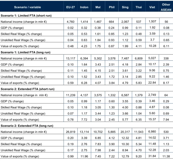
National Income Changes
The results as illustrated in Table 2., show that intra-regional trade liberalisation can be expected to deliver positive net income effects on all the economies involved under all the scenarios envisaged in this study. Throughout the study, some negative outcomes are registered for other ASEAN countries (i.e. Brunei, Cambodia, Laos & Myanmar) which are consistent with the results of other CGE studies in other trade liberalisation experiments.
As theory predicts, the income gains raises in tandem with the degree of liberalization, and also more in the long-run where capital accumulation effects are taken into account. There is, in fact, a significant leap in income effects as we move to different scenarios and between the short and long-run. The EU and Singapore gain the most, followed by ASEAN’s biggest country, Indonesia. In GDP growth terms, however, the FTA is mostly beneficial for Vietnam. Even in the most conservative short-run scenario, Vietnam experiences almost a 2 percent GDP increase, over and above the 8 percent baseline growth (see Table ). It is worth noting that most of ASEAN reaps considerable growth premiums in the long-run even in the most limited trade liberalisation experiment.
Table 2.1.1
National Income changes (mln Euro) and GDP percentage growth
Scenario / variable EU-27 Indon Mal Phil Sing Thai Viet Other ASEAN Limited FTA (short run)
National income
(change in mln €) 4,761 1,414 1,467 664 2,067 537 1,507 56 GDP (% change) 0.02 0.32 0.38 0.24 0.99 0.11 1.92 0.08
Limited FTA (long run)
National income
(change in mln €) 13,117 6,394 5,302 3,576 7,487 6,809 5,027 338 GDP (% change) 0.10 1.64 3.43 2.51 4.18 2.84 10.17 2.39
Extended FTA (short run)
National income
(change in mln €) 11,239 4,137 3,575 1.332 6,587 1,379 2,749 64 GDP (% change) 0.05 0.99 1.17 0.60 3.55 0.39 3.46 0.29
Extended FTA (long run)
National income
(change in mln €) 26,819 13,114 10,702 5 885 20,317 11,543 6,980 530 GDP (% change) 0.20 3.39 6.85 4.12 12.32 4.81 14.02 3.71
Extended FTA Plus (short run)
National income
(change in mln €) 12,021 3,706 3,852 1.530 7,125 1,490 2,621 154 GDP (% change) 0.06 0.88 1.22 0.63 3.66 0.36 3.22 0.27
Extended FTA Plus (long run)
National income
(change in mln €) 29,516 14,207 11,714 7 196 21,507 13,061 7,637 725 GDP (% change) 0.23 3.66 7.42 5.02 12.89 5.39 15.27 4.39
Source: ICE model simulations
To trace the underlying reasons for these gains from trade, these (long-run) income effects are further decomposed according to each trade liberalization measure, i.e., import protection in goods, barriers to trade in services, and other non-tariff barriers to trade. These are summarized in Table 2.1.2 below.
Table 2.1.2
Decomposition of Dynamic Real Income Effects (million EUR, 2007)
Measure
Scenario Country Tariffs Services NTB Total
EU 5,597 5,068 2,452 13,118
Indonesia 3,038 2,343 1,014 6,395
Malaysia 2,260 1,988 1,054 5,302
Measure
Scenario Country Tariffs Services NTB Total
Singapore 723 5,421 1,344 7,488 Thailand 3,998 1,466 1,346 6,810 Vietnam 4,007 449 572 5,028 Other ASEAN 164 19 156 339 EU 6,737 14,857 5,225 26,820 Indonesia 3,377 7,716 2,022 13,115 Malaysia 2,493 6,124 2,087 10,703 Philippines 2,268 1,216 2,401 5,885 Singapore 763 16,999 2,556 20,317 Thailand 4,473 4,349 2,722 11,543 Vietnam 4,414 1,423 1,143 6,980 Ambitious FTA Other ASEAN 164 47 321 531 EU 6,973 14,963 7,580 29,517 Indonesia 3,499 7,650 3,058 14,207 Malaysia 2,546 6,068 3,100 11,714 Philippines 2,356 1,198 3,642 7,197 Singapore 781 16,842 3,884 21,508 Thailand 4,610 4,321 4,130 13,061 Vietnam 4,513 1,399 1,726 7,637 Ambitious Plus FTA Other ASEAN 188 46 491 726
As can be expected, the gains from pure tariff liberalization are largely exhausted in the limited FTA scenario. But especially for Singapore and the EU, it is the considerable reduction in the barriers to Services Trade that matters the most, as it account for 78 percent and 51 percent of the total income gains, respectively, for the most ambitious liberalisation experiment. After the EU, it is Thailand that gains the most from the removal of non-tariff barriers. Given the relative underdevelopment of Services in other ASEAN countries, it is not surprising that removal of protection leads to some income losses for the said economies. The income gains accruing from trade facilitation is visible from the changes in the share of incomes due to NTB liberalisation under the ambitious FTA and ambitious plus FTA scenarios. For instance, for the EU about 87 percent of the income rise between these two scenarios is due to direct and indirect effects of trade facilitation alone.
Wage effects for low- and high-skilled workers
The productivity effects of intra-regional trade liberalization surface here in the form of rising wages for all economies involved. Given the significant wage differentials between the EU and ASEAN across all class of workers, the relatively higher wage effect for ASEAN is to be expected. This result is not trivial if one takes into account the weak presence of labour unions, and the relatively high unemployment rates in ASEAN. The more marked increase in Singapore wages, however, is likely a scarcity issue given its small labour market and its tight labour immigration policies especially for unskilled workers.
Table 2.1.3
Real wage effects on EU and ASEAN Unskilled Workers (% change)
Short run/ Static effects Long Run/ Dynamic Effects
Limited FTA Ambitious FTA Ambitious Plus FTA Limited FTA Ambitious FTA Ambitious Plus FTA EU 27 0.04 0.07 0.08 0.1 0.17 0.19 Indonesia 0.63 1.17 1.15 1.52 2.75 3.01 Malaysia 1.84 3.44 3.72 3.43 7.98 8.7 Philippines 0.93 1.23 1.35 1.72 2.44 2.86 Singapore 1.12 3.66 3.86 3.14 8.94 9.36 Thailand 0.59 1.04 1.06 2.85 4.7 5.23 Viet Nam 3.68 5.6 5.5 9.22 12.28 13.3 Other ASEAN 0.65 0.69 1.08 1.46 2.03 2.72
Source: ICE Model simulations
Table 2.1.4
Real wage effects on EU and ASEAN Skilled Workers
Short run/ Static effects Long Run/ Dynamic Effects
Limited FTA Ambitious FTA Ambitious Plus FTA Limited FTA Ambitious FTA Ambitious Plus FTA EU 27 0.05 0.1 0.1 0.11 0.19 0.21 Indonesia 0.53 1.18 1.09 1.45 2.76 3.02 Malaysia 1.61 3.05 3.31 4.15 7.83 8.56 Philippines 0.85 1.3 1.56 2.51 3.9 4.84 Singapore 1.23 4 4.29 3.61 10.3 10.84 Thailand 0.48 0.88 0.91 3.22 5.34 6.02 Viet Nam 3.59 4.87 4.78 9.06 11.48 12.61 Other ASEAN 0.13 0.08 0.46 0.75 1.13 1.73
Source: ICE Model simulations
Change in value of Exports
ASEAN exports will register a significant increase, with Vietnam seeing a 10 percent rise in exports even under a limited short-run scenario. On average, exports will rise in the long-run by about 14 percent, fuelled by the performance of ASEAN’s new Member States, i.e., Vietnam (35 percent), and Laos & Myanmar (15 percent). The EU likewise benefits from higher exports, albeit to a more modest degree.
Table 2.1.5
Change in Export values (in %)
Short run/ Static effects Long run / Dynamic Effects
Limited FTA
Ambitious FTA
Ambitious
Plus FTA Limited FTA
Ambitious FTA
Ambitious Plus FTA
Short run/ Static effects Long run / Dynamic Effects Indonesia 4.23 7.72 8.35 6.28 11.96 13.07 Malaysia 1.75 3.04 3.49 4.07 7.45 8.32 Philippines 0.87 2.45 3 3.84 7.22 8.95 Singapore 1.99 5.77 6.09 4.79 12.79 13.82 Thailand 4.11 6.35 7.15 5.83 9.2 10.29 Vietnam 10.28 15.37 16.1 22.84 31.84 34.86 Other ASEAN 6.11 7.94 8.89 8.17 11.38 13.02
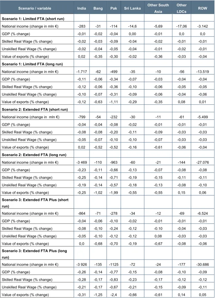
Global (third country) Effects
As earlier mentioned, a free trade area that includes countries with high initial protection typically generates a net result of trade diversion. In the EU-ASEAN FTA case, however, the generally negative third-country effects portrayed in Table 2.1.6 is largely the effect of the reduction of EU protection vis-à-vis ASEAN exports, and more especially in the range of products where ASEAN directly competes with South Asian goods. However, one must note that even in the scenario where the potential of trade diversion is the greatest, the effects are negative but rather trivial. Under the most ambitious trade liberalization scenario between the EU and ASEAN, it is Pakistan’s exports that are largely affected, with its exports falling by 2.4 percent. The extent of trade diversion for the rest-of-the world is indeed minimal, as exports fall by a mere 0.05 percent.
Table 2.1.6
Summary of Macro Economic Changes, Rest-of-the-World (ROW)
Scenario / variable India Bang Pak Sri
Lanka Other South Asia Other LDCs ROW
Scenario 1: Limited FTA (short run)
Nat'l. income (change in mln €) -283 -31 -114 -14.6 -5.69 -17.06 -3,142 GDP (% change) -0.01 -0.02 -0.04 0.00 -0.01 0.0 0.0 Skilled Real Wage (% change) -0.02 -0.03 -0.09 -0.04 -0.02 -0.01 -0.01 Unskilled Real Wage (% change) -0.02 -0.04 -0.05 -0.04 -0.01 -0.02 -0.01 Value of exports (% change) 0.02 -0.35 -0.30 -0.02 -0.36 -0.03 -0.04 Scenario 1: Limited FTA (long run)
Nat'l. (change in mln €) -1.717 -62 -499 -35 -10 -56 -13.519 GDP (% change) -0.11 -0.06 -0.34 -0.07 -0.03 -0.04 -0.04 Skilled Real Wage (% change) -0.12 -0.06 -0.36 -0.10 -0.06 -0.05 -0.05 Unskilled Real Wage (% change) -0.10 -0.07 -0.31 -0.09 -0.06 -0.04 -0.06 Value of exports (% change) -0.12 -0.63 -1.11 -0.29 -0.35 0.08 0.01 Scenario 2: Extended FTA (short run)
Nat'l. income (change in mln €) -799 -54 -232 -30 -11 -61 -5 499 GDP (% change) -0.04 -0.04 -0.08 -0.02 -0.01 -0.01 -0.01 Skilled Real Wage (% change) -0.08 -0.08 -0.20 -0.11 -0.09 -0.03 -0.03 Unskilled Real Wage (% change) -0.05 -0.07 -0.10 -0.10 -0.07 -0.03 -0.03
Scenario / variable India Bang Pak Sri Lanka Other South Asia Other LDCs ROW
Scenario 2: Extended FTA (long run)
Nat'l. income (change in mln €) -3.469 -110 -963 -60 -21 -144 -27 076 GDP (% change) -0.23 -0.11 -0.66 -0.13 -0.07 -0.08 -0.08 Skilled Real Wage (% change) -0.25 -0.14 -0.71 -0.19 -0.15 -0.11 -0.11 Unskilled Real Wage (% change) -0.19 -0.14 -0.57 -0.18 -0.13 -0.08 -0.10 Value of exports (% change) -0.25 -1.02 -1.99 -0.55 -0.55 0.15 0.06 Scenario 3: Extended FTA Plus (short run)
Nat'l. income (change in mln €) -864 -71 -278 -34 -12 -69 -6.524 GDP (% change) -0.04 -0.06 -0.10 -0.02 -0.01 -0.01 -0.01 Skilled Real Wage (% change) -0.08 -0.10 -0.24 -0.12 -0.10 -0.04 -0.03 Unskilled Real Wage (% change) -0.05 -0.10 -0.12 -0.12 0.08 -0.03 -0.03 Value of exports (% change) 0.0 -0.68 -0.70 -0.19 -0.67 -0.08 -0.06 Scenario 3: Extended FTA Plus (long run)
Nat'l. income (change in mln €) -3.926 -135 -1.125 -72 -24 -177 -30 686 GDP (% change) -0.26 -0.14 -0.77 -0.15 -0.08 -0.10 -0.09 Skilled Real Wage (% change) -0.28 -0.17 -0.83 -0.23 -0.17 -0.12 -0.12 Unskilled Real Wage (% change) -0.21 -0.17 -0.67 -0.21 -0.15 -0.09 -0.11 Value of exports (% change) -0.31 -1.25 -2.4 -0.66 -0.61 0.14 0.05
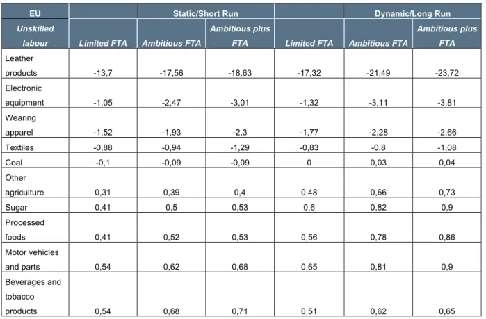
2.2 Sectoral effects
EU-27
The detailed impact on sectors for the EU is provided in the set of Tables in the Annex. For this section we limit the analysis to sectors were changes in output, prices, exports, imports, and employment appear to be significant.
The sectors that matter for the EU are those in the area of Services, and these sectors all expand under all possible scenarios. Although the changes in percentage terms appear small, their large shares in total output translate these changes into more significant revenues for EU Service providers. This is particularly true for trade services, other business services, which each take up about 10 percent of total EU27 output.
Under manufacturing sectors, the reduction in output is evident in leather products (-24 percent), clothing (-3 percent), and electronic equipment (-4 percent). These effects are expected as trade liberalisation unleashes the dynamic effects of competition, (negatively) positively affecting sectors of comparative (dis)advantage. Hence, EU Services and ASEAN (more labour-intensive) Manufacturing sectors expand as a result of free intra-regional free trade.