Wind tunnel experiments on the optimization of
distributed suction for laminar flow control
M C M Wright¤andP A Nelson
Institute of Sound and Vibration Research, University of Southampton, UK
Abstract: It is well known that surface suction can delay boundar y layer transition from laminar to turbulent flow, thus reducing drag on the surface in question. In order for laminar flow control by means of suction to be a paying proposition on aircraft, however, it must reduce total energy consumption as well as net drag. The flow control system that will have the best chance of doing this will use the minimum amount of suction pump energy to achieve a given transition position. Previous work has shown how a steepest-descent constrained optimization algorithm in conjunction with a radial basis function gradient estimator is capable of doing this online. In this paper the control strategy is applied to a large (2 m chord, 1.6 m span) aerofoil model in a low turbulence tunnel, with variable incidence and direct force measurement. The effect of pressure gradient over the suction section on the efficacy of the suction can therefore be observed, as can the relationship between transition and drag. The system is shown to converge reliably as long as the desired transition is within its range, and to be capable of maintaining control after a change in aerodynamic conditions without needing to re-identify the gradient estimation coefficients.
Keywords:drag, boundar y layer, suction, transition, optimization
NOTATION
Cd drag coefficient Cp pressure coefficient Cv suction coefficient e transition position error
g pump energy cost k time step index
N number of suction panels r desired transition position U1 freestream flow velocity v suction velocity
v vector of suction velocities
y transition position
á angle of incidence
â error reduction parameter
ì Lagrange multiplier
í step size parameter = vector derivative operator
Superscript
T transpose of a vector
1 INTRODUCTION
Hybrid laminar flow control is being considered as a viable means of reducing direct operating costs (DOC) for commercial aircraft [1–3], the rationale being that the application of suction to a limited region of a wing or nacelle can maintain laminar flow over a substantial portion of the chord, thus reducing drag and therefore energy consumption by the propulsion system in steady flight. Since the suction system consumes energy, the contribution to a reduction in DOC will therefore be the difference between the propulsion energy saved and the pump energy spent. Proposed suction systems have multiple, independent suction panels [4], meaning that different suction distribu-tions with different pump energy consumption can produce the same transition position and hence the same propulsion energy saving. In order to be able to choose the suction condition that will lead to the greatest saving in DOC it is necessary to be able to minimize pump energy while maintaining any particular transition position. Of course, many other factors that determine DOC will also be affected by the introduction of suction, such as cleaning and maintenance costs, change in fuel load, etc. (discussed in references [1] to [3]), and these must be considered when deciding upon the overall feasibility of laminar flow The MS was received on 31 July 2000 and was accepted after revision for
publication on 10 September 2001.
¤Correspondin g author: Institute of Sound and Vibration Research, University of Southampton , Highfield, Southampton SO17 1BJ, UK.
control. These factors, however, are outside the scope of this paper which examines a method for minimizing pump energy expenditure.
Previous work has shown that this requirement can be formulated as an equality-constrained optimization subproblem, and an algorithm based on the steepest-descent method with gradient projection has been devel-oped to solve it adaptively [5]. This algorithm has been shown to work on a small, fixed wind tunnel model with four suction panels [6], and the algorithm was subsequently modified to use a neural network based gradient estimator for faster convergence [7]. In this paper, experiments are reported in which this algorithm was applied to a large aerofoil model in a low-turbulence wind tunnel, which allowed variable incidence (and hence pressure gradient) and direct measurement of drag forces.
2 APPARATUS
2.1 Wing model
The wing section was symmetrical so as to have nominally zero lift at zero incidence with suction on one side only. The section was based on a NACA 66012 aerofoil [8] of 1 m chord, but with an additional 1 m flat section inserted
at the point of maximum thickness, giving a thickness ratio of 6 per cent and a total chord of 2 m. The NACA 66012 profile was chosen because:
1. It is symmetric so that introducing the flat section would not interrupt the flow.
2. It is reasonably thick so as to allow room for the suction boxes inside the aerofoil.
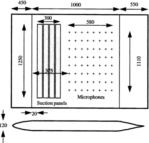
The span was 1.6 m. The purpose of this design procedure was to allow the suction and transition detection to operate on a flat surface so as to obviate the need to manufacture curved suction boxes, while allowing natural laminar flow to a point downstream of the suction application. Owing to the weight limit of the force balance in the tunnel, the model was of a wooden construction, over which a stainless steel skin was fitted on the active side by AS&T Limited. The skin extended over the stagnation point to the inactive side to ensure smooth leading edge flow, and was perforated at the section lying over the suction boxes. The suction boxes were designed to produce uniform suction in the spanwise direction, but with four independent controls in the chordwise direction. Full dimensions of the model are given in Fig. 1. The porosity of the surface was tested before fitting and found to be such that a pressure drop of 3736 N=m2 induced an average flow velocity of 0:3 m=s
through the skin. The perforation pattern was deliberately
Fig. 1 Layout of the wing model (all dimensions in millimetres)
random so as to avoid generating periodic structures in the boundary layer, but typical hole dimensions were of the order of 100ím.
An undesirable consequence of the wood –metal con-struction was that the different thermal expansivities induced a certain degree of waviness in the active side of the model. The wave amplitude was typically 2 mm, and the average wave length typically 200 mm. Any departure from flatness would be expected to have the effect of locally altering the pressure gradient and hence the rate of change of transition with suction. Since the aim of these experiments is not to compare measured transition with that predicted by any theory, this waviness cannot be said to induce errors as such. It will, however, have an effect on the function that must be minimized in order to control the transition, which will be to make it less smooth that it would be with a perfectly smooth model. Any control algorithm, therefore, that can successfully control transition on this model should be able to do so at least as well, if not better, on a smoother model. In preliminary trials, side pieces having the same cross-section as the wing were fitted to the tunnel walls with a gap of approximately 2 mm between each side piece and the model, in order to maintain two-dimensional flow over the wing surface. These proved difficult to align, and for the experiments reported here the wing was fitted with side fences, flow visualization using woollen tufts having confirmed that the flow over the sucked span of the active surface was unchanged. The small increase in drag owing to the addition of the side fences was amply repaid by the ease with which incidence could be adjusted. The wind speed was 20 m=s for all tests.
2.2 Suction pump system
Each of the four individual suction compartments was connected to an ESAM Uni-Jet 40 CE 250 W side-channel aspirator pump via a Microbridge AWM5103V air flow sensor with a range of 0–20 L=min (standard litres per minute), corresponding to a range of suction velocities of 0–3:6 mm=s, or a nominal maximum velocity coefficient ofCvˆv=U1 ˆ1:8310¡
4. The speed of each pump was
controlled from a PC via a Eurotherm type 601 three-phase inverter. In principle it was possible to use an integral control loop to set each pump to suck at a desired suction velocity. In practice, for extensive testing the convergence time of this ‘inner-loop’ control was found to be too slow. Instead, the pump was calibrated against the flow meter over its range at the start of each test, and thereafter the appropriate pump voltages were determined by interpola-tion in a look-up table, which allowed the maximumCv to be extended somewhat beyond the nominal value given above.
2.3 Transition detection system
The flat section also had an 838 array of miniature electret microphones mounted behind 0.5 mm holes at
locations shown in Fig. 1, which were used to detect the surface pressure fluctuations and hence distinguish between laminar and turbulent regions. The holes behind which the microphones were mounted were distinct from the pressure tappings used to measure the static pressure distribution. The microphone signals were high-pass filtered at 800 Hz to remove any tunnel noise by a bank of filters and preamplifiers manufactured in-house. The signals were then acquired and averaged by the PC. Forty microphones at a time could be monitored (five streamwise rows), the extra microphones being provided so that, if a microphone failed during the experiment, a spare streamwise row could easily be substituted. The r.m.s. pressures were normalized to the level measured with no suction and a turbulent boundar y layer over all microphones. The estimated transition displacement was then taken to be the sum of all the normalized pressures when the suction was applied, divided by the number of chordwise microphone rows in operation (to give the average transition displacement in ‘number of microphones’), multiplied by the spacing between microphones (83 mm) to give a displacement in metres. The number of microphones needed on a full-scale aircraft implementation would depend on the precision with which it was necessary to control the transition, which in turn would depend on the cost benefit analysis for that particular aircraft. The EU HYLDA project, under which this work was funded, considered the possibility of applying such a system to an engine nacelle, for which, typically, 30 microphones might be necessary. Of course, the control procedure described herein could equally be applied with any other transition detection system.
2.4 Control system
The system was controlled by a rack-mounted PC fitted with three LSI TMS320C40 data acquisition boards. The signals from the flow meters and the microphone formed the inputs, and the control voltages to the pump inverters formed the output. For reasons discussed in the introduc-tion, the control algorithm attempts to adjust a vector of suction velocities so as to drive the difference between the measured and desired transition positions while minimizing a model of the energy consumed by the pumps, assumed here to be the sum of the squares of the suction velocities. No attempt was made to correlate this with the actual electrical power consumed by the pumps, since the pumps had not been designed for this application as would be the case with an aerospace installation, and therefore could not be assumed to be operating under efficient conditions. Nonetheless, there is no reason why a more sophisticated system could not optimize against a more sophisticated or realistic model of energy consumption. The optimization algorithm updates the vector of suctions,v, according to
vk‡1ˆvk¡í=(gk‡^ìkek) (1)
where g is the modelled energy cost, e is the difference between actual and desired transition position and
^ ìkˆ f[¡í=gT k=ek‡(1¡â)ek]=(í=eTk=ek)g ‡^ìk¡1 2 (2)
The gradients are estimated from a radial basis function (RBF) model of the suction error function identified at the start of each run as described in reference [7].
3 EXPERIMENTAL PROGRAMME
3.1 Pressure measurements
A detailed preliminary investigation of the pressure distribution over the unsucked model was made at zero incidence and corrected for blockage effects by measuring the ambient pressure along a streamwise line mid-way between the model and the floor of the tunnel. This showed (unsurprisingly for such a simple geometry) that the pressure distribution was completely in accordance with that predicted by a simple panel method calculation. Subsequent pressure profile measurements were not ad-justed in this manner and therefore represent the actual pressure experienced along the surface of the model. The
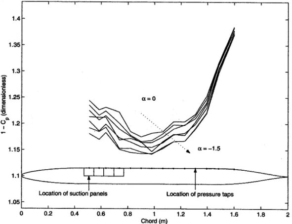
static pressure taps were located at the points indicated in Fig. 2, referenced to a stagnation pressure in the free-stream.
Seven incidence conditions were employed for each phase of the tests, namelyáˆ0,¡0.25,¡0.5,¡0.75,¡1, ¡1.25 and ¡1.58. In general, as will be seen, and as is expected, the effect of makingámore negative is to make it easier for the suction to delay the transition point. Figure 2 shows the variation in pressure gradient with incidence measured from the front suction box to the back micro-phone with no suction applied.
3.2 Uniform suction tests
Figures 3 to 5 show how drag coefficient (normalized to the frontal area of the model) and transition vary with suction applied uniformly over all four suction compart-ments, and how the drag coefficient varies with transition under these conditions. The values at whichCvdata points occur on different traces do not line up together owing to the interpolation procedure referred to above. Clearly, the zero incidence case has an added drag component, other-wise all expected trends are followed. In subsequent tests where non-unifor m suction distributions were employed, the drag was assumed to vary with transition position in a similar manner to that shown in Fig. 5, since it was possible to measure and record transition automatically with the suction control computer located above the tunnel, whereas
Fig. 2 Variation in pressure distribution with angle of incidence (negativeácorresponds to the nose moving down)
Fig. 3 Variation in drag with uniform suction for various incidences
Fig. 4 Variation in transition displacement with uniform suction for various incidences
drag had to be measured on a separate system located in the wind-tunnel control room. The departure of the traces in Fig. 4 from smooth curves may be due to the waviness of the surface referred to above.
3.3 Exhaustive suction distribution tests
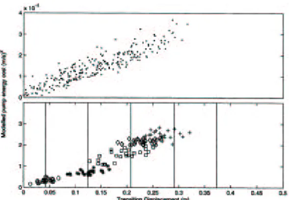
For each incidence, the suction distribution was system-atically stepped through all possible combinations of four values of Cv, giving a total of 44ˆ256 different suction
distributions. Figure 6 shows scatters of the correspond-ing model energy g versus the resulting transition displacement for three of the incidence conditions. Once again, as expected, an increase in negative incidence produces more transition delay for a given expenditure of suction energy. This figure also reveals, however, that the difference in suction energy consumption for a given transition position of the best and worst suction distribu-tions is more than a factor of 2 for most of the range of most cases.
3.4 Control/optimization tests
The optimization procedure was implemented for each of the incidence cases, and the optimization algorithm was applied for 100 iterations for each of five target transition displacements, corresponding to the first five microphone
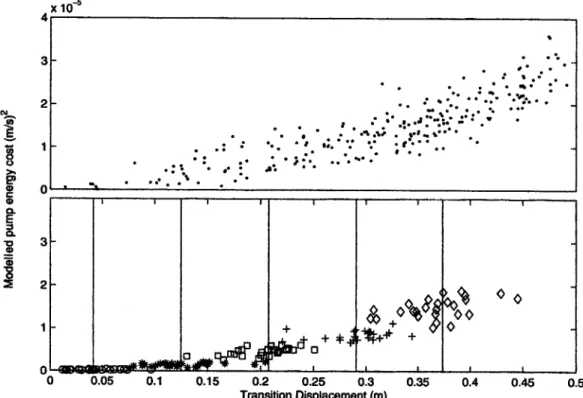
locations. The transition histories for three incidence conditions are shown in Figs 7 to 9. The modelled pump energy that was required to be minimized at each transition location was also recorded, and these results can best be appreciated in the context of the scatter plot format already employed. Figures 10 to 12 show the controlled transition cost scatters for iterations 75 to 100 for the same cases, each symbol corresponding to a successive run, starting from the same initial condition but with a different desired transition position. The values for iterations 75 to 100 were plotted because after 75 iterations any transient due to the controller converging had died out, as can be seen from Figs 7 to 9. Increasing the number of iterations would therefore have had no effect. Comparison of these figures with the corresponding exhaustive scatters in the upper plots of these figures shows the success of the algorithm in that the ‘cloud’ of optimized points lies at the bottom of the corresponding cloud for exhaustive suction distribu-tions (implying minimization of cost) horizontally centred on the required transition position (implying control of transition position). This is only so, however, when the desired transition lies within the attainable range of the system, as can be seen from Fig. 10. Comparison with the following two figures shows that the run indicated by the diamond symbols is attempting to maintain the transition at the furthest chosen desired transition. As can be seen from the upper trace, this transition is unattainable by any Fig. 5 Variation in drag with transition displacement, uniform suction varying along joined lines for various incidences
Fig. 6 Transition cost scatters for three incidences
Fig. 7 Transition histories during control,ሠ¡0:258(dashed lines show desired transition positions)
Fig. 8 Transition histories during control,ሠ¡0:758(dashed lines show desired transition positions)
Fig. 9 Transition histories during control,ሠ¡1:258(dashed lines show desired transition positions)
Fig. 10 Exhaustive (upper) and optimized (lower) transition cost scatters,ሠ¡0:258. Each symbol corresponds to a separate run with a different desired transition (shown by vertical line)
Fig. 11 Exhaustive (upper) and optimized (lower) transition cost scatters,ሠ¡0:758
Fig. 12 Exhaustive (upper) and optimized (lower) transition cost scatters,ሠ¡1:258
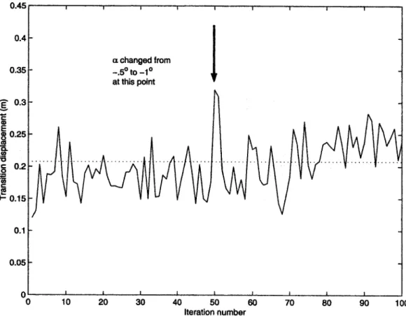
Fig. 13 Transition history during control, with change in incidence
suction distribution, and under these conditions the algorithm settles for a transition position that is less than it is possible to achieve because of its requirement to minimize cost. The increasing size of the ‘clouds’ of controlled points on these plots indicates that the accuracy with which both transition and cost variables can be controlled decreases the longer the laminar portion of the boundary layer is required to be.
3.4.1 Transient response of the optimization system A potential disadvantage of the RBF-based gradient estimator is that it identifies (albeit crudely) the suction transition response at one particular aerodynamic condi-tion, and, if that condition changes during the subsequent control phase, then a mismatch between the true and estimated gradients might cause the system to become unstable or misadjusted. In order to test this, the identifica-tion and control procedure described above was implemen-ted as before, but after 50 iterations the incidence was changed fromሠ¡0:58 toሠ¡18. The procedure was then repeated with the incidence changing fromሠ¡18to
ሠ¡0:58. The resulting transition histories are shown in Figs 13 and 14. It can be seen that, while the control after the change in conditions is not as regular as it was before, it is still stable and well behaved. In Fig. 13, for instance, the transition after the change in incidence is delayed from the
desired control point somewhat. This is not surprising, since the plant model is now different from that being used by the controller, nonetheless the change in attained transition point is small and, after about 30 iterations, stable. Of course, this does not guarantee a similar response for all possible changes in conditions, but it does indicate that the control system is not sensitive to arbitrarily small disturbances.
4 CONCLUSIONS
The results presented demonstrate that the suction optimi-zation system based on the previously reported optimiza-tion algorithm with a radial basis funcoptimiza-tion gradient estimator is capable of minimizing suction energy while maintaining constant transition position. This system has been physically realized and applied to a 2 m chord wind-tunnel model which has been tested at the University of Southampton in a 79 359wind tunnel at a flow speed of 20 m=s. It has been established that the system converges to the required state over a range of incidence angles and target transitions positions, and that the system is robust to changes in aerodynamic conditions.
Fig. 14 Transition history during control, with change in incidence
ACKNOWLEDGEMENTS
This work was supported by the European HYLDA project sponsored by the European Union (Contract BE95-1084). The model and control system were built, installed and operated by Messrs A. E. Sanger, D. J. Goldsworthy, D. K. Edwards, G. Baldwin, M. Tudor-Pol e and A. R. Edgely.
REFERENCES
1 Joslin, R. D. Aircraft laminar flow control. Ann. Rev. Fluid Mechanics, 1998,30, 1– 29.
2 Denning, R. M., Allen, J. E. andArmstrong, F. W. Future large aircraft design—the delta with suction. Aeronaut. J., 1997,101(1005), 187 –198.
3 Wilson, R. A. L. andJones, R. I. Laminar flow for subsonic
transport aircraft.Aerospace Engng, June 1996,16(6), 21 – 25. 4 Bieler, H., Pfennig, J. and Herrmann, R. A320 HLF fin:
Interdisciplinary approach to a boundary layer suction system. In 2nd European Forum on Laminar Flow Technology, Paris, 1996, pp. 7.48– 7.56 (Association Ae´ronautique et Astronau-tique de France).
5 Nelson, P. A., Wright, M. C. M.andRioual, J.-L.Automatic control of boundary-layer transition. Am. Inst. Aeronaut. Astronaut. J., 1997,35(1), 85 –90.
6 Wright, M. C. M. and Nelson, P. A. Four-channel suction distribution optimization experiments for laminar flow control.
Am. Inst. Aeronaut. Astronaut. J., January 2000,38(1), 39– 43. 7 Wright, M. C. M. and Nelson, P. A. Fast boundary layer
suction optimisation with neural networks. Proc. Instn Mech. Engrs, Part G, Journal of Aerospace Engineering, 2000,
214(G2), 107 – 113.
8 Abbott, I. H. and von Doenhoff, A. E. Theory of Wing Sections, 1959 (Dover).