A Survey on Efficient Hashing Techniques in Software Configuration Management

A Survey on Efficient Hashing Techniques in

Software Configuration Management

Bernhard Grill

Vienna University of Technology Vienna, Austria

Email: [email protected]

Abstract—This paper presents a survey on efficient hashing techniques in software configuration management scenarios. Therefore it introduces in the most important hashing techniques as open hashing, separate chaining and minimal perfect hashing. Furthermore we evaluate those hashing techniques utilizing large data sets. Therefore we compare the hash functions in terms of time to build the data structure, performing only successful lookups and performing only unsuccessful lookups. The results indicate that minimal perfect hashing clearly outperforms the other presented hashing techniques.

I. INTRODUCTION& OVERVIEW

This paper presents an overview on efficient hashing tech-niques in software configuration management (CM) settings. Software configuration management tools store the configura-tion for an executable, e.g. configuraconfigura-tion file and command line parameters. Therefore such systems typically utilize key-value stores. An example for such a CM is Elektra [19]. It’s widely known that hashing techniques represent an efficient way to handle key-value pairs in relation to lookup times. Therefore this paper focus on different hashing techniques applicable in CM settings.

First the paper introduces the most important hashing tech-niques as open hashing, separate chaining and minimal perfect hashing. Section II has a detailed look into open hashing techniques like linear probing, quadratic probing, double and Cuckoo hashing. Section III outlines separate chaining tech-niques, in particular we tackle exact fit and move to front technique. Perfect hashing and especially minimal perfect hashing are discussed in Section IV. Section V compares the presented hashing techniques in terms of storing large data sets, while Section VI concludes the paper.

The most important aspect of hash functions is their be-havior in terms of collisions i.e. when two keys both try to occupy the same hash table location. In general there are two techniques how to deal with collisions. The first one is to handle the occurring conflicts while the second technique is to completely avoid collisions. Figure 1 outlines the most important hashing data structures and surveys their behavior. Open hashing utilizes a probing function for collision resolution which is invoked until an empty position in the table is found. The basic idea of separate chaining techniques is to apply linked lists for collision management, so in case of a conflict the new key is appended to the linked list. The idea of minimal perfect hashing is to always map distinct elements to

distinct hash table positions without any collisions by creating a custom hashing function perfectly fitting the used key set.

II. OPENHASHING

This section outlines a survey on the most effective open hashing techniques. Open hashing (also known as open ad-dressing) is a technique utilizing an additional probing func-tion for collision resolufunc-tion. Whenever a hash collision occurs the probing function is invoked until either the target key is located or an empty record is found i.e. indicating the requested key is not existent. In the following we will discuss the most important probing functions:

• Linear probing [15] - Section II-A

• Quadratic probing [15] - Section II-B • Double hashing [15] - Section II-C • Cuckoo hashing [18] - Section II-D

A. Linear Probing

The principle of linear probing is accomplished by utilizing a start index, determined by h(k), and a stepping value i, wherehis the hashing function andkis the new key to insert. The starting index is determined by the hash function h(k), whereasicontains the stepping interval which is continuously added, until a free key is found in the hash table or the whole table is passed through:iis typically a relative prime number to the hash table’s size m, in order to ensure the whole table is traversed. The position for a key utilizing linear probing is computed by:h(k, i) = (h(k) +i)mod m

When the stepping valueiis equals one, the probing function selects consecutive positions in the hash table. Double hash-ing is a type of linear probhash-ing utilizhash-ing a hash function to determinei.

The performance for linear probing depends on the amount of probes fired during a key search, which depends on the hash table’s load factor α=n/m, where nis the number of occupied entries andm the hash table’s size. The higher the hash table’s load factorαthe higher is the amount of probes performed. According to Knuth [15] the estimated average number of probes operated by linear probing is given by 1₂(1+

1 1−α).

Typically hardware architecture dependent parameters, like the cache size, have significant performance impacts on hash-ing techniques. Several contributions [2], [7], [13], [21], [23]

Fig. 1. Examples for minimal perfect hashing (a), open hashing techniques (b) and chaining techniques (c) [8]

show the impact of caching on open hashing and separate chaining techniques.

B. Quadratic Probing

Quadratic probing is highly related to linear probing. The position for a key is computed by: h(k, i) = (h(k) +c1i+

c2i2)mod m. The hash functionh(k)determines the position

for key k. The hash table’s size is given by m, whereas i is the probe position for the key k and c1 and c2 are constant

values [15].

Heileman et al. showed that linear probing has a better performance than quadratic probing in settings where the entire hash table does not fit into the cache memory [13]. On the other hand quadratic probing has a better perfor-mance in scenarios with high hash table load factors α. This characteristic is based on the improved clustering nature of linear probing compared to quadratic probing. Though linear probing typically produces more probing attempts than quadratic probing, those attempts feature a very high cache hit rate resulting in a better overall performance in practice when the whole hash table doesn’t fit in the cache memory. In settings where most of the hash table resides in cache memory, quadratic probing techniques like [15] or [16] outperform linear hashing procedures. The outperformance is based on the fact that most of the probes are cache hits and quadratic probing produces less probing attempts than linear probing. On the other hand quadratic probing shares some drawbacks with linear probing, e.g. the high search costs for tables with hash table load factors α close to 1 [14]. According to Knuth [15] the following equation calculates the estimated average number of probes performed for a key search utilizing quadratic probing: 1−ln(1−α)−α

2.

C. Double Hashing

Double hashing utilizes two hash functions h1 and h2.

Whileh1 calculates the start index for the key,h2determines

the step value in case of a collision. Using double hashing a key’s position is computed as follows: h(k, i) = (h1(k) +

i∗h2(k))mod m [15]. The other parameters are defined as

before.

Double hashing effectively tackles clustering problems oc-curring in linear and quadratic probing, as the second hashing functionh2provides varying step values for each key.

Further-more multi-collision settings produce a Further-more homogeneous key distribution than linear or quadratic probing. Double hashing still shares some problems with the afore mentioned techniques as increased search costs for hash tables with a high load factorα. According to Knuth [15] the estimated average number of probes for a key search using double hashing is given by−1

αln(1−α).

D. Cuckoo Hashing

The name Cuckoo hashing refers the cuckoo bird, where baby cuckoos push other chicks out of their nest after hatching. In terms of hashing a new key may push an existing key to a different position in the hash table. It utilizes two hash functionsh1(k)andh2(k). Whenever a new keykis inserted,

either the position computed by h1(k) or h2(k) is chosen.

When the chosen position is already occupied by keyk2, the key k2 will be replaced by k. Then the replaced key k2 has two possible new locations as well, defined by h1(k) and

h2(k). One of those two possible locations will be used as

new position fork2. If both locations fork2are occupied the procedure is repeated until each pushed key is inserted or the key can not be inserted anymore [10], [18].

The replacement behavior may result in an infinite loop as cycles may appear during insertion. Infinite loops can be prevented by permitting only a certain amount of iteration cycles. Nevertheless, in this case the hashing technique won’t be able to insert the key, before the entire hash table is rebuild with two different hash functionsh1(k)andh2(k).

Figure 2 outlines the functionality ofCuckoohashing by an example. The arrows indicate the alternative positions of each key. Consider a new item would be inserted in the location of key ”A”. Therefore the existing key ”A” is moved to its alternative position, at the moment taken by key ”B”. Now key ”B” has to be pushed to its alternative position which is currently unoccupied. Inserting a new item currently occupied by ”H” would not succeed, as key ”H” and ”W” build a cycle, kicking each other endlessly.

Fig. 2. Explanation on the functionality of cuckoo hashing [1]

though considering the scenario to rebuild the entire hash table as long as the table’s loadαes kept below 50% [18] .

Erlingsson et al. proposed a generalized Cuckoo hashing technique which can handle hash table’s load up to 99% [10]. The idea is to utilize not only two hash functions but an arbitrary amount of different hashing functions. The more different hashing functions are applied, the higher is the resulting maximum load factor αof the hash table.

Ross et al. proposed performance improvements for the generalized Cuckoo hashing technique by applying single-instruction-multiple-datastream (SIMD) instructions to exploit parallelisms and eliminate branch instructions within the prob-ing functions [21].

III. SEPARATECHAINING

The basic idea of separate chaining techniques is to uti-lize additional data structures, e.g. linked lists, for collision resolution. Each hash table key has its own list for collision resolution. The advantage of chaining techniques relies in the ability to easily resolve conflicts and the permanent possibility to insert new keys without resizing the hash table. Hence, applying separate chaining techniques may result in hash table load factors α beyond 1, which is impossible for open hashing techniques. On the other hand chaining techniques may result in drastic performance penalties when the hash table degenerates, e.g. to a linked list. Such a degeneration may also increase the cache miss rates dramatically [7]. In the following we will discuss the two most important chaining techniques:

• Move to front [22] - Section III-A • Exact fit [15] - Section III-B

A. Move to Front

The move to front technique consists of the hash table and a linked list for each key to handle the collisions. Whenever a conflict in a hash table key occurs, the new key is appended to the list’s end. The core idea of this technique is whenever

a key is accessed it is moved to the beginning of the linked list.

In case of searching a key in the hash table’s conflict reso-lution list, the same parts of memory are accessed repeatedly. The move to front technique exploits the locality by moving recently used keys to the front of the list. This technique speeds up the future search for the same key. Hence, frequently accessed keys tend to occupy positions at the beginning of the list, while rarely used ones are typically stored at the list’s end. This behavior reduces the average lookup time for keys. B. Exact Fit

The exact fit technique provides a cache-aware option for separate chaining technique. It keeps an array of neighboring entries instead of a linked list for colliding keys per hash table item. Therefore this method is able to exploit higher memory locality than techniques applying linked lists, where items are typically stored in random memory locations. Hence, the array entries for conflict resolution are stored in a contiguous way in memory, resulting in less cache misses and decreased lookup time. Fibure 3 outlines a hash table exploiting the exact fit technique.

Fig. 3. Hash table applying exact fit technique [8]

The benefit of the exact fit technique is simultaneously a drawback as the technique requires storing colliding hash table entries in a contiguous way. Thus inserting a new value can results in allocating memory and copying the old array’s content to the new contiguous location.

Askitis et al. have shown that applying the exact fit tech-nique in settings with variable length keys can result in heavy performance impacts [2].

IV. PERFECTHASHING

The basic idea of perfect hashing is to avoid collisions at all. Perfect hash functions map a static key set of n entries to a set of m numbers without any collision. In other words they map distinct elements to distinct hash table positions without collisions at all times for static key sets. Therefore such techniques do not have to implement collision resolutions techniques. In mathematical terms, perfect hashing techniques apply total injective functions. In the following we will discuss minimal and order preserving perfect hash functions.

Minimal perfect hash functions (MPH) map different keys exclusive of any collisions and without leaving any position inbetween unoccupied. In other words if n (the number of entries for the static key set) is equal tom(the number of hash table entries) the function is called a minimal perfect hashing function. Figure 4 outlines the difference between perfect hash functions and minimal perfect hash functions. Whereas perfect hash functions map keys to hash table positions without any collisions, minimal perfect hash functions additionally produce consecutive entries in the hash table without leaving any location vacant.

Minimal perfect hash functions are often used for fast lookup and memory efficient storage of static key sets. Ex-amples for such static key sets are URLs in online web search engines, words for languages (both natural and programming languages) or configuration parameters for software programs. Furthermore MPH functions are highly relevant as indexing data structure in database applications as shown by Botelho in [8]. Typically B+ trees are used for indexing in database systems. B+ trees are beneficial in highly dynamic scenarios with numerous insert and remove operations on the data structure. However B+ trees are not suitable in scenarios with little change and a massive amount of entries, as those data structures perform poorly and are highly complex to administrate in large key set scenarios. In areas like database systems, big data or business intelligence working with huge data structures is daily business. For example assigning ids to a collection of URLs might be challenging, as database systems utilizing traditional data structures might collapse once the working set for the URLs does not fit into the main memory anymore. On the other hand minimal perfect hashing functions can easily handle up to hundred of million entries in memory using standard commodity hardware, due to their dense data structure. [20]

Order preserving minimal perfect hash functions addition-ally preserve the order of keys in subject to a function f. E.g. consider the following keys a1, a2, ..., an; given any

keys aj and ak (j < k) implies f(aj) < f(ak). Such

hashing techniques require necessarily Ω(n log n) bits to be represented [11].

Fig. 4. Comparing perfect hash functions (a) and minimal perfect hash functions (b) [20]

As perfect hash functions do not suffer from collisions or unoccupied positions within their data structures, such hashing

functions have to be generated individually to fit the desired key set. Therefore hash function generators are utilized to create the proper fitting perfect hash function for the favored key set. Those generators use the desired key set as input to construct the fitting hash function.

Fredman et al. and Melhorn et al. introduced perfect hash functions in their publications in 1984 [12], [17]. In the same year Fredman et al. proved that minimal perfect hash functions require at least n log e + log u − O(log n) bits [12]. Also in 1984 Melhorn et al. provided a minimal perfect hashing function [17] nearly satisfying the lower bound proposed by Fredman et al. [12]. His hashing function requires at most

n log e+log u+ O(log n)bits. Belazzougui et al. proposed methods to create monotone minimal perfect hash functions [4], [5]. The minimal perfect hash functions proposed by Botelho et al. are the best in term of lookup time and storage space [9]. Those require about 2.62 bits per key [3], [9]. In 2009 Belazzougui et al. discovered a fundamental lower bound for minimal perfect hashing functions which require minimum 1.44 bits per key [6].

V. HASHPERFORMANCECOMPARISON

In 2011 Botelho et al. evaluated the performance of dif-ferent hash function types [8]. In this section we present an aggregation and discussion on those results.

The experiments were performed on Linux 2.6, with an Intel Core 2 processor @1.86 GHz, 4 GB of main memory and 4 MB L2 cache. The results are averages on 50 repetitions and were statistically validated with a confidence level of 95%.

They used three different key sets for evaluation. The first consists of 5,424,923 unique queries from a online search engine, subsequent referred asWebQ. The second and third key set contain 10 million respectively 37,294,116 unique URLs, henceforth calledURLs-10andURLs-37.

In the following we will compare the performance of open hashing techniques in Section V-A and Cuckoo hashing, separate chaining and perfect hashing techniques in Section V-B.

A. Comparing Open Hashing Techniques

This section compares the performance of open hashing techniques except ofCuckoo hashing because the number of probing attempts were not measured for Cuckoo. Cuckoo’s performance is evaluated in Section V-B.

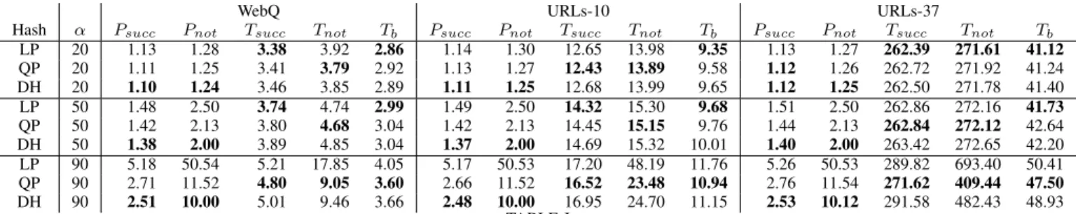
Table I gives a survey on the hash table’s load factor α

(in percent of the hash table’s size) impact on the times (in seconds) to successfullyTsucc respectively unsuccessfully

Tnotlookup keys. The evaluation utilizes linear probing (LP),

quadratic probing (QP) and double hashing (DH) techniques. It looks up 10, 20 respectively 250 million keys in theWebQ, URLs-10 respectivelyURLs-37 key set applying load factors ranging from 20% to 90%. The evaluation considers both successful Tsucc and unsuccessful Tnot lookup times for all

queries.Psucc indicates the average number of probes per key

for the scenario only processing successful lookups, whereas

WebQ URLs-10 URLs-37

Hash α Psucc Pnot Tsucc Tnot Tb Psucc Pnot Tsucc Tnot Tb Psucc Pnot Tsucc Tnot Tb

LP 20 1.13 1.28 3.38 3.92 2.86 1.14 1.30 12.65 13.98 9.35 1.13 1.27 262.39 271.61 41.12 QP 20 1.11 1.25 3.41 3.79 2.92 1.13 1.27 12.43 13.89 9.58 1.12 1.26 262.72 271.92 41.24 DH 20 1.10 1.24 3.46 3.85 2.89 1.11 1.25 12.68 13.99 9.65 1.12 1.25 262.50 271.78 41.40 LP 50 1.48 2.50 3.74 4.74 2.99 1.49 2.50 14.32 15.30 9.68 1.51 2.50 262.86 272.16 41.73 QP 50 1.42 2.13 3.80 4.68 3.04 1.42 2.13 14.45 15.15 9.76 1.44 2.13 262.84 272.12 42.64 DH 50 1.38 2.00 3.89 4.85 3.04 1.37 2.00 14.69 15.32 10.01 1.40 2.00 263.42 272.65 42.20 LP 90 5.18 50.54 5.21 17.85 4.05 5.17 50.53 17.20 48.19 11.76 5.26 50.53 289.82 693.40 50.41 QP 90 2.71 11.52 4.80 9.05 3.60 2.66 11.52 16.52 23.48 10.94 2.76 11.54 271.62 409.44 47.50 DH 90 2.51 10.00 5.01 9.46 3.66 2.48 10.00 16.95 24.70 11.15 2.53 10.12 291.58 482.43 48.93 TABLE I

PERFORMANCE COMPARISON BETWEEN LINEAR PROBING,QUADRATIC PROBING AND DOUBLE HASHING UTILIZING DIFFERENT HASH TABLE LOAD FACTORSα,DATA FROM[8]

lookups only scenario. Furthermore the table outlines the time

Tbin seconds to build the hash structure. The bold items mark

the best values per category.

In general, linear probing performs pretty well in terms of average probing attempts per lookup (Psucc,Pnot) and time

for a successful or unsuccessful search (Tsucc, Tnot) in case

of low and medium load factors (α = 20, α = 50). But its performance declines sharply when applying high load factors. Furthermore the amount of probing attempts per key access (bothPsuccandPnot) increases dramatically for linear probing

in high load settings. This behavior indicates massive troubles for the technique to deal with clustering in the hash table’s data structure.

Double hashing clearly outperforms linear and quadratic probing in terms of probing attempts per lookup (both Psucc

andPnot). On the other hand double hashing is slower in case

of average time spent for successfully looking up the keys (Tsucc) compared to quadratic probing.

Linear probing shows the best performance in terms of time to build the hash data structure Tb in case of low or medium

load factors (α= 20,α= 50). Whereas quadratic probing has the best performance with high load factors.

The average number of probing attempts (Psucc andPnot)

are close to the expected numbers according to the presented equations in Section II. Table II compares the calculated and observed average number of probing attempts. The calculation for the observed average number of probes is based on the results from Table I.

Probing technique α Observed avg. probes Calculated avg. probes Deviation (%) LP 20 1.13 1.13 0.00 LP 50 1.49 1.50 0.66 LP 90 5.20 5.50 5.45 QP 20 1.12 1.12 0.00 QP 50 1.43 1.44 0.69 QP 90 2.71 2.85 4.91 DH 20 1.11 1.12 0.89 DH 50 1.38 1.39 0.72 DH 90 2.51 2.56 1.95 TABLE II

COMPARING THE OBSERVED AND CALCULATED AVERAGE NUMBER OF PROBING ATTEMPTS

Interestingly the observed average amount of probing at-tempts is always lower or equal than the calculated one. In

general it differs the most when applying high load factorsα. B. Comparing Cuckoo Hashing, Separate Chaining and Per-fect Hashing Techniques

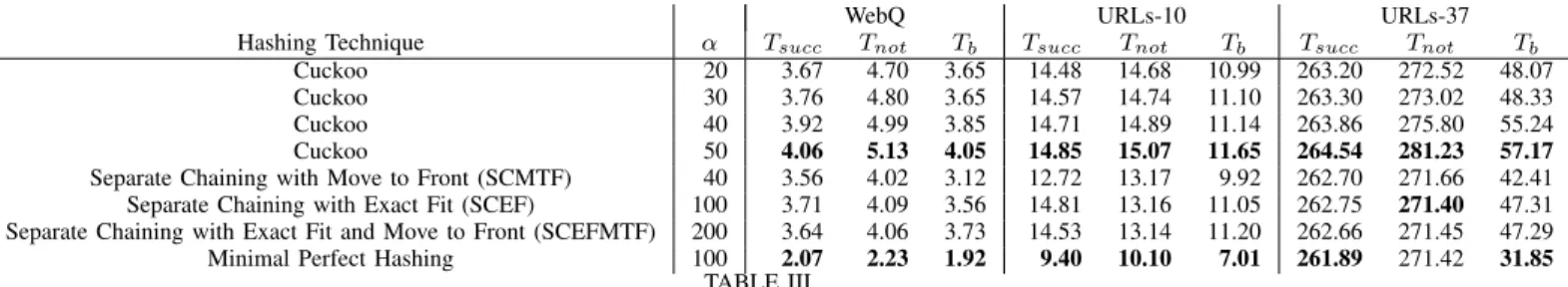
This section compares the performance of the remaining hashing techniques asCuckoohashing (CuH), separate chain-ing with move to front (SCMTF), separate chainchain-ing with exact fit (SCEF), separate chaining with exact fit and move to front (SCEFMTF) and minimal perfect hashing (MPH) which are outlined in Table III. The parameters have the same meaning as in Table I.

AsCuckoohashing can not operate on load factors>50%, the evaluation outlines the results for load factors between 20% and 50% (indicating maximum possible load).

Table III shows very interesting results. The bold items mark the best and the worst values per column. The hash table’s build time Tb for minimal perfect hashing (MPH) is

extraordinary fast compared to the other techniques, as it does not need to handle any collisions. When the data structure MPH fits into the L2 cache, which applies in case ofWebQand URLs-10 key set, it significantly outperforms other hashing techniques. This observation applies for both successful and unsuccessful scenarios (Tsucc andTnot). In the contrary

situ-ation, where the hashing data structure doesn’t fit into the L2 cache, the performance is pretty similar among the investigated hashing techniques in both successful and unsuccessful lookup settings. Altogether MPH either outperforms or in worst case has similar performance results as the other hashing techniques have.

In case of low hash table load factors Cuckoo hashing has related performance characteristics as the other hashing techniques. But in high load factor scenarios Cuckoo’s per-formance significantly declines in both settings. Notably, the chaining techniques don’t suffer as much performance impact in high load factor scenarios as open hashing techniques do (compare Table I and III). Interestingly the performance of separate chaining with exact fit and move to front (SCEFMTF) does not decline on high load factors, on the contrary it has the lowest minimum lookup time (except of MPH) for the URLs-37 key set. The reason is the dense hashing data structure caused by the high load factor which additionally benefits from caching effects compared to sparse data structures. This observation does not hold for successful lookup times Tsucc

WebQ URLs-10 URLs-37 Hashing Technique α Tsucc Tnot Tb Tsucc Tnot Tb Tsucc Tnot Tb

Cuckoo 20 3.67 4.70 3.65 14.48 14.68 10.99 263.20 272.52 48.07

Cuckoo 30 3.76 4.80 3.65 14.57 14.74 11.10 263.30 273.02 48.33

Cuckoo 40 3.92 4.99 3.85 14.71 14.89 11.14 263.86 275.80 55.24

Cuckoo 50 4.06 5.13 4.05 14.85 15.07 11.65 264.54 281.23 57.17

Separate Chaining with Move to Front (SCMTF) 40 3.56 4.02 3.12 12.72 13.17 9.92 262.70 271.66 42.41 Separate Chaining with Exact Fit (SCEF) 100 3.71 4.09 3.56 14.81 13.16 11.05 262.75 271.40 47.31 Separate Chaining with Exact Fit and Move to Front (SCEFMTF) 200 3.64 4.06 3.73 14.53 13.14 11.20 262.66 271.45 47.29 Minimal Perfect Hashing 100 2.07 2.23 1.92 9.40 10.10 7.01 261.89 271.42 31.85

TABLE III

PERFORMANCE COMPARISON ONCuckooHASHING,MOVE TO FRONT,EXACT FIT,EXACT FIT AND MOVE TO FRONT AND MINIMAL PERFECT HASHING,

DATA FROM[8]

of separate chaining with exact fit (SCMTF) since it can’t exploit caching so well, due to the random memory accesses performed during linked list traversal.

Although MPH functions show a clear outperformance compared to other hashing techniques, it has the drawback of being only able to handle static key sets which results in recreating the MPH function on each configuration parameter change. Generating the MPH function to utilize the WebQ, URLs-10 and URLs-37 key set took 9.57, 21.81 respectively 95.48 seconds. This observation shows a nearly linear scale in terms of the key size for the MPH function’s generation time. The performance gain is based on the MPH function’s ability to find any key in the table via one single probe and its great cache memory exploitation behavior due to extremely dense hash data structures.

VI. CONCLUSION

In general linear probing (LP) performs pretty well in scenarios with low hash table loadsα. While quadratic probing (QP) outperforms LP when applying high load to the hash table, double hashing (DH) has the lowest amount of probing attempts throughout the evaluation of open hashing techniques. Cuckoo hashing, Separate Chaining with Exact Fit (SCEF) and Separate Chaining with Exact Fit and Move to Front (SCEFMTF) performed rather poor compared to the other techniques.

Minimal perfect hashing (MPH) clearly outperforms all the other presented techniques. The performance gain is based on MPH’s ability to find any key via one single probe and its great cache memory exploitation behavior due to extremely dense hash data structures. Therefore MPH clearly outperforms the other techniques in scenarios where the whole data structure fits into the CPU cache. Furthermore MPH has by far the lowest build time Tb for the hash data structure during the

evaluation. Although MPH functions are only able to handle static key sets, which results in recreating the MPH function on each configuration parameter update, they clearly beat the other hashing techniques presented in this paper and are therefore the best hashing technique in software configuration scenarios.

REFERENCES

[1] Cuckoo hashing. http://programmingpraxis.com/2011/02/01/cuckoo-hashing/, 2011, Last Accessed: 2014-10-11.

[2] N. Askitis and J. Zobel. Cache-conscious collision resolution in string hash tables. InString Processing and Information Retrieval, pages 91– 102. Springer, 2005.

[3] M. J. Atallah. Algorithms and theory of computation handbook. CRC press, 1998.

[4] D. Belazzougui, P. Boldi, R. Pagh, and S. Vigna. Monotone minimal per-fect hashing: searching a sorted table with O(1) accesses. InProceedings of the twentieth Annual ACM-SIAM Symposium on Discrete Algorithms, pages 785–794. Society for Industrial and Applied Mathematics, 2009. [5] D. Belazzougui, P. Boldi, R. Pagh, and S. Vigna. Theory and practice of monotone minimal perfect hashing. Journal of Experimental Algo-rithmics (JEA), 16:3–2, 2011.

[6] D. Belazzougui, F. C. Botelho, and M. Dietzfelbinger. Hash, displace, and compress. InAlgorithms-ESA 2009, pages 682–693. Springer, 2009. [7] J. R. Black, C. U. Martel, and H. Qi. Graph and hashing algorithms for modern architectures: Design and performance. In Algorithm Engineering, pages 37–48, 1998.

[8] F. C. Botelho, A. Lacerda, G. V. Menezes, and N. Ziviani. Minimal perfect hashing: A competitive method for indexing internal memory. Information Sciences, 181(13):2608–2625, 2011.

[9] F. C. Botelho, R. Pagh, and N. Ziviani. Simple and space-efficient minimal perfect hash functions. In Algorithms and Data Structures, pages 139–150. Springer, 2007.

[10] U. Erlingsson, M. Manasse, and F. McSherry. A cool and practical alternative to traditional hash tables. In Proc. 7th Workshop on Distributed Data and Structures (WDAS06), 2006.

[11] E. A. Fox, Q. F. Chen, A. M. Daoud, and L. S. Heath. Order-preserving minimal perfect hash functions and information retrieval. ACM Transactions on Information Systems (TOIS), 9(3):281–308, 1991. [12] M. L. Fredman and J. Koml´os. On the size of separating systems and families of perfect hash functions.SIAM Journal on Algebraic Discrete Methods, 5(1):61–68, 1984.

[13] G. L. Heileman and W. Luo. How caching affects hashing. In ALENEX/ANALCO, pages 141–154, 2005.

[14] F. Hopgood and J. Davenport. The quadratic hash method when the table size is a power of 2. The Computer Journal, 15(4):314–315, 1972. [15] D. Knuth. The art of computer programming: Sorting and searching,

volume 3, chapter 6.3, 1998.

[16] W. Luo and G. L. Heileman. Improved exponential hashing. IEICE Electronics Express, 1(7):150–155, 2004.

[17] K. Mehlhorn. Sorting and Searching, volume 1 of Data Structures and Algorithms. Springer, 1984.

[18] R. Pagh and F. F. Rodler. Cuckoo hashing. Journal of Algorithms, 51(2):122–144, 2004.

[19] M. Raab. Elektra initiative - libelektra. https://github.com/ElektraInitiative/libelektra, Last Accessed: 2014-10-11.

[20] D. d. C. Reis, D. Belazzougui, F. C. Botelho, and N. Ziviani. Minimal perfect hashing. http://cmph.sourceforge.net/, Last Accessed: 2014-10-11.

[21] K. A. Ross. Efficient hash probes on modern processors. In ICDE, pages 1297–1301, 2007.

[22] J. Zobel, S. Heinz, and H. E. Williams. In-memory hash tables for accumulating text vocabularies. Information Processing Letters, 80(6):271–277, 2001.

[23] M. Zukowski, S. H´eman, and P. Boncz. Architecture-conscious hashing. InProceedings of the 2nd international workshop on Data management on new hardware, page 6. ACM, 2006.