Abstract— This report describes the process and benefits of a Monte-Carlo approach for analyzing uncertainty in an information security investment. The Monte-Carlo approach captures uncertainty in security modeling parameters (vulnerabilities, frequency of intrusion, damage estimates, etc) and expresses its impact on the model’s forecast (e.g. projected benefit). The forecast is presented as a chart understandable by controllers and middle-level managers responsible for resource allocation decisions. This approach is especially valuable for visualizing a potentially large return on an investment that defends against an unlikely but catastrophic attack.
Index Terms— Monte-Carlo methods, reliability, Risk analysis, Security.
I. INTRODUCTION
HEN information security investments compete for resources with other more concrete business opportunities, the security analyst may need to help the financial decision makers position the value of security within their familiar terms. But the uncertainties of information security modeling parameters (vulnerabilities, frequency of intrusion, damages, effectiveness of mitigations, etc) frustrate this discussion. So many things might happen. On the other hand, the decision makers may well understand that a new piece of equipment must be acquired to support an alternative business opportunity. What they may not know is the likelihood that the benefits of this equipment will be rendered irrelevant by a successful cyber attack. How can the security officer communicate this risk when so little is known to be certain? This report describes how to employ a Monte-Carlo simulation with an information security risk model to better visualize the potential of an information security investment.
Monte-Carlo simulations are of course not new. However, Monte-Carlo software has matured during the past decade to where commercial off-the-shelf tools [1] [2] [3] enable nearly anyone skilled in spreadsheet development to construct a Monte-Carlo simulation. In addition, financial decision makers may already be familiar with Monte-Carlo simulations so we are “speaking their language” when we apply them to analyzing information security risks.
Information security risk models often employ expected
Manuscript received March 3, 2005.
J. R. Conrad is a doctoral student with the University of Idaho, Moscow, ID 83844 USA (e-mail: conr2286@uidaho.edu).
values in their parameters that assume each quantity is known. But this approach fails to capture uncertainty in the modeling parameters. For example, an expert might estimate the frequency of a particular attack to be 2 intrusions per year. Could it be only 1 intrusion per year? Perhaps. Could it be 4? Sure. Is 4 more probable than 1? Well, yes. How about 100? No, that would be unlikely. A Monte-Carlo simulation enables an analyst to quantify the uncertainty in an expert’s estimate by defining it as a probability distribution rather than just a single expected value.
Uncertainty in modeling parameters can arise from either of two sources, a truly random process or from an expert’s lack of understanding of an underlying process. When a distinction is helpful, this report adopts the terminology of Vose [4] to distinguish between variability (the result of a random process) and uncertainty (the analyst’s lack of understanding). While better estimates might reduce the uncertainty in a forecast, they cannot reduce its variability. Vose proposes techniques for separating uncertainty from variability that this report will forego.
Finally, please note that the Monte-Carlo approach is not a new security model --- it’s an alternative approach for applying an existing model that enables the analyst to work with random variables.
II. PRIOR WORK
FIPS65, an early United States study of the need for information security in large data centers, estimated risk as a financial metric, the Average Loss Expectancy (ALE), calculated as the sum of the products of annual consequences (dollars) and frequencies of occurrence [5]. Soo Hoo observes that ALE’s reliance on expected values dangerously equates high-probability but low impact events with low-probability but catastrophic events [6]. He also notes that ALE-based risk models become overly complex when they attempt to address all threats, assets and vulnerabilities.
Considerable recent work has focused on securing critical infrastructures (energy, telecommunications, health-care, finance, transportation, etc). This need is documented by Oman [7] and Longstaff who describes a simple efficacy model for analyzing the return on an information security investment for a financial infrastructure [8]. Taylor et al. examine an approach for hardening electrical power substations using quantified cost/benefit results [9]. Geer explains the need to use Return On Investment (ROI) [10] for information risk management decisions.
Analyzing the Risks of Information Security
Investments with Monte-Carlo Simulations
James R. Conrad,
Member, IEEE Computer Society
Schechter [11] introduces a market-based approach to evaluate the strength of a secured system as the market price for discovering the next new vulnerability. Schechter argues that the strength of a system’s security should be quantified from the viewpoint of the attacker rather than the defender. In this context, he concludes the strength of a system with known vulnerabilities is negligible.
Butler et al. champion the use of portfolio analysis [12] for guiding software investment (including security) decisions. Soo Hoo recommends a stochastic approach [6] (of which
Monte-Carlo is an example) to study the role of uncertainty. Many information security models are described in the literature. Some take a low-level approach [13] and model the network structure as a graph, often focusing on the underlying vulnerabilities by modeling the route of attack. Other models
adopt a systems-level approach [5] [6] [8] [9] that abstracts the many details of the underlying network in favor of focusing on the higher-level risks with less regard for the route of attack. Information security models quantifying risks as financial values are often implemented at the systems-level.
In order to illustrate the process and benefits of the Monte-Carlo approach, two example simulations will be constructed using Longstaff’s efficacy model [8]. The simplicity of this particular model is ideal for this purpose as it avoids distracting attention from exploring the Monte-Carlo approach. Although many information security models are much more complex, the Monte-Carlo approach will scale using commercial tools. The reader is encouraged to evaluate the Monte-Carlo approach with their security risk model.
Longstaff’s efficacy example calculates the value of a security investment as a benefit/cost ratio where 1.0 is breakeven and bigger is better. The example uses the parameter estimates of Table I and is replicated here to validate the Monte-Carlo implementation. The efficacy model calculates five intermediate results and forecasts the benefit/cost ratio (R) of a proposed information security investment as shown in Table II. Longstaff illustrates the use of the efficacy model with a financial infrastructure example that forecasts the expected value of the benefit/cost ratio (R) of the proposed investment to be 7.22. A Monte-Carlo simulation of this example should provide a comparable
expected value of the resulting forecast.
III. MONTE-CARLO SIMULATION OVERVIEW
In a Monte-Carlo simulation (Fig. 1), the security model is treated as a function passed a set of parameters and returning a set of forecasted results. Rather than supplying a single set of fixed parameter values directly to the security model, the analyst defines a set of random variable distributions (the expert’s estimates) to the Monte-Carlo tool. When the simulation is run, the tool selects a random value for each parameter, executes the hosted security model with those values, and collects the forecasted results from the model. Selection, execution and collection are repeated in many (often thousands of) iterations of the model. Commercial Monte-Carlo tools offer a capability to display the result of the simulation as a chart plotting the forecast’s distribution.
Please note that an existing security model may not need to be re-designed to manipulate random variables; it continues to operate on fixed values as always. The Monte Carlo tool simulates the random variables by repeatedly executing the model. The only required modification to the model may be to link its input and output to the Monte Carlo tool. TABLE I
EFFICACY MODEL PARAMETERS
Param Description Units Estimates p1 Likelihood of successful
intrusion without risk assessment
intrusions/day .00548 p2 Likelihood of successful
intrusion with risk assessment
intrusions/day .00274
X Value of Assets $/day 20E12
y1 Cost of software assurance
without risk assessment $/year 100E6 y2 Cost of software assurance with
risk assessment
$/year 200E6 z1 Losses without risk assessment %Assets 1% z2 Losses with risk assessment %Assets 0.5%
TABLE II
EFFICACY MODEL CALCULATIONS
Calculation Description Units d1 = p1*z1 Losses without risk assessment %Assets d2 = p2*z2 Losses with risk assessment %Assets D = y2 – y1 Cost to provide software
assurance with risk assessment $ d = d1 – d2 Losses prevented by risk
assessment
%Assets B = d*X-D Net benefit of risk assessment Dollars R = (d*X-D)/D Forecasted benefit/cost ratio
for risk assessment
Variable Distributions Monte-Carlo Simulation Tool Forecast Distribution Information Security Model
Depending upon the tool, the input parameters are linked using either a user interface dialog or (as illustrated in this report) using functions exported by the tool. Output results may also be linked with a user interface but the exact details depend upon the tool in use.
Before the analyst constructs a simulation, there is one caution that merits immediate discussion. A simulation requires each iteration of the model to be supplied with wholly independent parameters, or the analyst must alternatively address the joint probabilities of any interrelated parameters. Let’s examine this restriction more closely. An analyst wishing to study the effect of variability in Longstaff’s p1 and
p2 parameters upon the forecasted benefit/cost ratio, R, might be tempted to treat p1 and p2 as two wholly independent random variables. Although the Monte Carlo tool will throw random numbers into both parameters, this approach leads to situations (iterations) in which the risk of a successful intrusion is higher with risk assessment than it would have been without (e.g. p2>p1)! If this does not make sense, then the analyst may wish to calculate p2=e*p1 by introducing a new parameter, e, to model the effectiveness (the relation between the two parameters) of the risk assessment investment as a function of the first parameter. The analyst could even employ a random variable (whose expected value is 0.5) to express the uncertainty in the estimate for e.
The interrelated parameter issue may be the trickiest obstacle encountered in the development of the analyst’s first Monte-Carlo simulation. The solution described above avoided the problem by expressing one parameter as a function of the other. Vose offers a cardinal rule to guide an analyst through this and related issues [4], “Every iteration of
a [Monte-Carlo] risk analysis model must be a scenario that could physically occur.” We cannot expect the security model to render meaningful forecasts if we allow the Monte-Carlo tool to supply it with parameters that don’t make sense in “the real world.”
IV. THE BANKING EXAMPLE
Fig. 2 illustrates the formulas in a Monte-Carlo implementation of Longstaff’s banking example constructed in a spreadsheet. The r1 variable is the input parameter and the resulting forecast appears in R. Note that the model includes only a single random variable, a Poisson distribution, to model the annual intrusion rate without risk assessment (r1). The choice of this Poisson distribution models Longstaff’s estimate of “at least two major intrusions per year… without [investment in] systemic risk assessment and management” and an assumption of continuous potential for intrusion. The objective is to reproduce Longstaff’s result in order to verify the Monte-Carlo simulation before extending it with a second example.
The RANDPOISSON(2.0) function returns a random number in a Poisson Distribution whose mean rate is 2.0 intrusions/year. The Monte-Carlo tool provides the RANDPOISSON function that supplies the model with random values for r1 selected from the Poisson distribution. Different tools will of course provide functions of different names; the function names (e.g. RANDPOISSON) used in this report are merely representative.
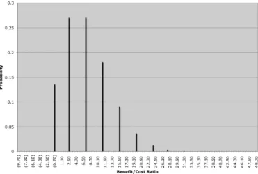
Fig. 3 illustrates the variability in the forecast resulting from executing the banking example simulation. The
Intrusion Rates
r1 =RANDPOISSON(2) Annual rate of intrusion w/o risk assessment investment
e 5.00E-01 Effectiveness of risk assessment investment
r2 =r1*e Annual rate of intrusion with risk assessment investment
Model Parameters
p1 =r1/365 Daily prob of intrusion w/o risk assessment investment
p2 =r2/365 Daily prob of intrusion with risk assessment investment
X $20,000,000,000,000 Asset value
y1 $100,000,000 Cost of software assurance w/o risk assessment investment
y2 $200,000,000 Cost of software assurance with risk assessment investment
z1 1.00% Losses w/o risk assessment
z2 0.50% Losses with risk assessment
Model Calculations
d1 =p1*z1 Calc damage w/o risk assessment investment
d2 =p2*z2 Calc damage with risk assessment investment
D =y2-y1 Calc cost to provide software assurance with risk assessment
d =d1-d2 Calc percentage of losses prevented by risk assessment investment
b =d*X-D Calc net benefit of risk assessment
R =b/D Calc benefit/cost ratio (Mean=7.22) for risk assessment investment
distribution takes on discrete values because the simulation modeled the r1 parameter with the discrete Poisson function: in any given year, there will be 0, 1, 2, 3… intrusions.
Fig. 3. Banking Example Forecast
In addition to the distribution, the Monte-Carlo tool also provides some statistics about the resulting forecast. The simulated mean value of the benefit/cost ratio (7.22) exactly equals that of the published banking example. Don’t expect them to always be equal though --- simulations are a random process! We must expect some minor variation. Given the various parameter estimates and the simulation assumption of a Poisson distribution for successful intrusions, the banking example anticipates a 25% chance of the benefit/cost ratio exceeding 11.3 and a 25% chance of the benefit/cost ratio being less than 3.11. There is also a 10% chance for a financial loss and a very remote chance for an extremely high benefit/cost ratio exceeding 30.
Fig. 4. Second Example Forecast
Why didn’t the simulation merely use the spreadsheet’s in POISSON function? Because the spreadsheet’s built-in function is not a source of random numbers as is the Monte-Carlo tool’s RANDPOISSON function. The RANDPOISSON function links the input of the security model to the Monte-Carlo tool. At the beginning of an iteration, the tool’s RANDPOISSON function supplies a new random value in the
r1 parameter. The Monte Carlo tool then has the spreadsheet
recalculate the model after which the tool captures the result (the benefit/cost ratio, R). The tool constructed Fig. 3 by simulating the random variables with 10,000 iterations.
Please note how straightforward it was to incorporate the efficacy model into a simulation. The RANDPOISSON function linked the model to a source of random numbers supplied by the Monte-Carlo tool, and the tool captured the result of each iteration from the R forecast. While different simulation tools handle the linking of parameters (with functions) and results (with a user interface) differently, the principle remains the same.
V. A SECOND EXAMPLE
The second example considers a case in which the hypothetical experts express two viewpoints about the annual rate of intrusion. The minority pessimistic view is the 2.0 estimate is historical and anticipated business conditions will cause it rise to 20.0 in the near future. The majority optimistic view is it will remain steady at 2.0. After substantial discussion, the experts concede there exists an 80% chance that the rate will remain the same and only a 20% chance that it will increase. The experts further agree that the rate will surely be one or the other but unlikely to be something in-between (perhaps the hypothetical experts cannot agree on the “anticipated business conditions”).
To model the experts’ uncertainty in this second example, the r1 variable is assigned the result from a discrete probability function (RANDDISCRETE) that selects the result of RANDPOISSON(2) 80% of the time (because the experts are 80% confident that the mean rate will remain at 2.0 intrusions/year) and selects the result of RANDPOISSON(20) 20% of the time (as the experts allow for a 20% possibility that the mean rate will rise to 20 intrusions/year). In each iteration of the simulation, the Monte-Carlo tool throws random numbers into both the optimistic (RANDPOISSON(2)) rate and the pessimistic rate (RANDPOISSON(20)), and then randomly selects one of the two possibilities for the r1 variable. The model simulates both the variability of the Poisson process and the uncertainty in the experts’ estimate of the mean intrusion rate.
Why didn’t the model simply calculate,
r1 = RANDPOISSON(2)*0.8+RANDPOISSON(20)*0.2 …rather than construct the more complicated simulation using RANDDISCRETE? The simple calculation would have discarded the bimodal nature (in the weighted average of the two Poisson variables) of the r1 distribution that was preserved with the RANDDISCRETE simulation function. In this example, the bimodal nature of r1 simulates the two conflicting expert opinions about the intrusion rate. Any attempt to conceal or “average away” this uncertainty conceals the truth: The experts don’t agree. A Monte-Carlo simulation preserves this uncertainty and reflects its impact upon the forecast.
Fig. 4 illustrates the bimodal forecast from this simulation where the effect of the two conflicting expert opinions is readily visible. The simulated expected value (mean) moves
up to 22, well above the 7.22 predicted in Fig. 3. The forecast also allows for a 10% possibility of the benefit/cost ratio exceeding 81 --- the expert’s uncertainty raises the forecasted probability of an extreme event. A risk-adverse financial decision maker concerned about the possibility of a catastrophe “on their watch” may wish to manage to the second mode. A risk-tolerant manager of a startup-up venture with more pressing issues at hand may be relieved to manage closer to the lower mode. This business decision should rightly be a function of an organization’s tolerance for risk but can be supported by the security analyst’s forecast illustrating the risks. A Monte-Carlo simulation of an information security model provides the decision makers with much more information than is available from a simple expected value.
Closer inspection of Fig. 4 reveals that although the location of the main mode remains in the same location as that of Fig. 3, it has become approximately twice as wide. Intuitively, the experts’ uncertainty about the intrusion rate erodes the model’s confidence in the width of the major mode.
Please note that the approach used above to express the expert’s uncertainty in the estimate of the average intrusion rate could also be used when the experts cannot even agree upon the right risk model! The simulation could execute multiple risk models and use a discrete probability function to randomly select one or another result.
The reader is encouraged to construct and experiment with this model by expressing additional uncertainty about the value of the e variable (effectiveness of risk assessment). Chances are, real experts would never agree that e is exactly 0.5000. The proposed investment might perform better than cutting the rate of successful intrusions by half. Or it might do worse. Your model could express that uncertainty and explore its impact upon the resulting forecast.
VI. CRITIQUE
The Monte-Carlo approach asks an expert to provide additional information about an estimate to describe its uncertainty. This additional information describes the shape and definitive parameters of an estimate’s distribution. But are real-world experts willing to comply? The author’s experience with Monte-Carlo applications is that many experts are in fact relieved to disclose the uncertainty they know to be in an estimate. What experts don’t like is being held accountable to a single expected value they know is merely representative of the possibilities.
VII. CONCLUSIONS
Monte-Carlo tools have matured and a wide range of commercial implementations is available to the security analyst. The Monte-Carlo approach is especially useful with systems-level information security models where it enables the analyst to express uncertainty in the experts’ estimates and illustrates the impact of that uncertainty on the resulting forecast. The additional information available from the forecasted distribution assists with the understanding of an
extreme event, the unlikely possibility of a catastrophic outcome.
REFERENCES
[1] Decisioneering. (2005, January 18). Crystal Ball. Available: http://www.decisioneering.com
[2] Palisade Corporation. (2005, January 18). @RISK. Available: http://www.palisade.com
[3] TreePlan. (2005, January 18). RiskSim. Available: http://www.treeplan.com/risksim.htm
[4] D. Vose, Risk Analysis --- A Quantitative Guide. West Sussex, England: John Wiley and Sons, 2000.
[5] National Bureau of Standards, Guideline for The Analysis Local Area Network Security, FIPS PUB 191, Washington DC: U.S. Government Printing Office, 1994, pp. 26-27.
[6] K. J. Soo Hoo, “How Much is Enough? A Risk-Management Approach to Computer Security,” Ph.D. dissertation, School of Engineering, Stanford University, Stanford, CA, 2000.
[7] P. Oman, E. Schweitzer III and D. Frincke, “Concerns About Intrusions into Remotely Accessible Substation Controllers and SCADA Systems,” in Proc. 27th Annual Western Protective Relay Conference, (Oct. 23-26,
Spokane, WA), 2000. Available: http://www.selinc.com/techpprs/6111.pdf
[8] T. Longstaff, C. Chittister, R. Pethia and Y. Haimes, “Are We Forgetting the Risks of Information Technology?,” Computer, IEEE, pp. 43-51, December 2000.
[9] C. Taylor, A. Krings and J. Alves-Foss, “Risk Analysis and Probabilistic Survivability Assessment (RAPSA): An Assessment Approach for Power Substation Hardening,” Proc. ACM Workshop on Scientific Aspects of Cyber Terrorism, (SACT), Washington DC, November 21, 2002.
[10] D. Geer Jr., “Making Choices to Show ROI,” Secure Business Quarterly, @stake, vol. 1, no. 2, Fourth Quarter, 2001, pp. 1-3. Available: http://www.sbq.com/sbq/rosi/sbq_rosi_making_choices.pdf
[11] S. Schechter, “Computer Security Strength & Risk: A Quantitative Approach,” Ph. D. dissertation, Computer Science, Harvard University, Cambridge, MA, 2004.
[12] S. Butler, P. Chalasani, S. Jha, O. Raz, M. Shaw, “The Potential of Portfolio Analysis in Guiding Software Decisions,” First Workshop on Economics-Driven Software Engineering Research, 1999. Available: http://www.cs.virginia.edu/~sullivan/EDSER-1/PositionPapers/jha.pdf [13] R. Lipton and L. Snyder, “A Linear Time Algorithm for Deciding
Subject Security”, Journal of the Association for Computing Machinery, vol. 24, no. 3, July 1977, pp. 455-464.