From Parameter Tuning to Dynamic Heuristic Selection

(1)

Fakultät Informatik Institut für Software- und Multimediatechnik, Lehrstuhl für Softwaretechnologie

From Parameter Tuning to

Dynamic Heuristic Selection

Yevhenii Semendiak

[email protected]

Born on: 7th February 1995 in Izyaslav, Ukraine Course: Distributed Systems Engineering

Matriculation number: 4733680 Matriculation year: 2017

Master Thesis

to achieve the academic degree

Master of Science (M.Sc.)

Supervisors

M.Sc. Dmytro Pukhkaiev

Dr. Sebastian Götz

Supervising professor

(2)

(3)

Abstract

The importance of balance between exploration and exploitation plays a crucial role while solving combinatorial optimization problems. This balance is reached by two general techniques: by using an appropriate problem solver and by setting its proper parameters. Both problems were widely studied in the past and the research process continues up until now. The latest studies in the field of automated machine learning propose merging both problems, solving them at design time and later strengthening the results at runtime. To the best of our knowledge, thegeneralizedapproach for solving the parameter setting problem in heuristic solvers has not yet been proposed. Therefore, the concept of merging heuristic selection and parameter control has not been introduced.

In this thesis we propose an approach for generic parameter control in meta-heuristics by means of reinforcement learning (RL). Making a step further, we suggest a technique for merging the heuristic selection and parameter control problems and solving them at runtime using RL-based hyper-heuristic. The evaluation of the proposed parameter control technique on a symmetric traveling salesman problem (TSP) revealed its applicability by reaching the performance of tuned in offline and used in isolation underlying meta-heuristic. Our approach provides the results on par with the best underlying heuristics with tuned parameters.

(4)

(5)

1 Introduction

1.1 Motivation

Heuristic-based optimization is a popular research area. Various optimization problems (OPs) are defined and can be tackled by heuristic algorithms [14, 43, 63]. Unfortunately, an ideal algorithm that can solve every OP does not and cannot exist. This issue was formalized by theno-free-lunch

theorem for optimization(NFLT) [121], which states that “all search algorithms have the same average performance over all possible optimization problems”. Heuristic solver acts by means ofexploration (effort diversification over a search space) andexploitation(effort intensification in a promising area) operations. The success of heuristic on the problem at hand is defined by the exposed strength of both operations (E&E) and the provided balance between them (EvE). Both E&E and EvE characteristics can be controlled in several ways.

Firstly, one could try to set proper values of hyper-parameters exposed by the algorithm. This process is formalized under the notion ofparameter settings problem(PSP), whose resolution can be done before running the algorithm (design time), or while it solves the OP (runtime). The former approach is also calledparameter tuningand can be tackled by numerous universal tuning systems [41, 58, 59, 79, 93]. A key assumption of this software is an expensive evaluation of the target system in terms of computational resources. High expensiveness is tackled by a surrogate learning model creation, which is then used to simulate the direct evaluations. The latter approach calledparameter controlwas originally introduced for evolutionary algorithms [66] and nowadays appears in analgorithm-dependentmanner. However, even a proper parameter setting may not lead to the best results for the problem at hand.

Secondly, one could try to select a proper algorithm. It was formalized as thealgorithm selection

problem(ASP) and defined as a process of searching for an appropriate solver for the problem at hand. ASP resolves the direct consequence of NFLT, which states that a single algorithm cannot be used to tackle various problems. Hyper-heuristics are commonly used for solving ASPs. They may perform low-level heuristic selection before solving [22] the actual problem, or at runtime [22]. To operate online, hyper-heuristics often utilize reinforcement learning (RL) techniques [84, 86], while for design time, a regular parameter tuning could be used.

The research has not been standing at a standstill and nowadays the researchers are actively attempting to merge ASP and PSP into a unitedalgorithm selection and parameter setting problem (APSP). For instance, in automatic machine learning such combination was formalized as thecombined algorithm

selection and hyper-parameter optimization problem (CASH) [112], while for heuristics the explicit studies of APSP merging and solving at runtime were not found. To tackle ML CASH problem several frameworks based on the existing parameter tuning systems were created [44, 88, 112]. However, those solutions are not applicable in case of heuristics, since they are (1) purely related to ML field and (2) acting at design time due to ML techniques nature. One may follow the ML approach of the united APSP search space definition and solving for heuristics, but it is applicableonlyat design time. Nevertheless, when it comes to runtime, it turns out that the universal technique for setting the parameters online (parameter control) in heuristics has not yet been proposed. It is essential, since the generic approach to tackle PSP is one of two required methodologies for solving heuristic APSP at runtime. The other building block (ASP) is already available in online hyper-heuristics.

(8)

1.2 Research objective

The goal of this thesis is to improve the quality of online heuristic-based optimization. The research objective is to determine whether it is possible to solve both PSP and ASP, while solving the OP. In order to reach our objective we need to answer the following research questions:

• RQ1Is it possible to perform the algorithm configuration at runtime on a generic level?

• RQ2Is it possible to simultaneously perform algorithm selection and parameters adaptation while solving an OP?

• RQ3What is the effect of selecting and adapting algorithms while solving an OP?

1.3 Solution overview

In this thesis we propose the unification of both ASP and PSP into a single problem. To do so, we firstly introduce a generic runtime PSP solution; secondly, we suggest joining several PSPs search spaces into a united APSP. The consequence of merging several PSPs into a single APSP is the appearance ofsparse search spaces, where the percentage of properly defined configurations is low due to requiring and prohibiting dependencies among parameters (e.g., each algorithm has its own required set of parameters).

To overcome the sparseness issue we propose a complex solution, which is spread in both search space structure and sampling process. For the APSP representation we suggest using a data structure, similar to feature trees from software product lines field. By doing so, we treat a solver type and its hyper-parameters uniformly. The dependencies between parameters are explicitly handled in the form of parent-child relationship. As a result, the search space could be viewed as a layered structure, where on the first level the algorithm type is defined, and on the level(s) below its respective hyper-parameters are specified. The prediction process is made sequentially for each level, utilizing the available performance evidence in a form of already tried configurations and respective improvements. Therefore, in the united APSP we firstly build a surrogate model for the algorithm type prediction. Afterwards, when the solver type is selected, we filter the performance evidence to operate on data, which is relevant to the selected algorithm type. With this filtered data we build a surrogate for the second level and predict the parameters values on second level. This level-wise process continues until obtaining a completed configuration. Next, we continue solving the underlying OP with the defined algorithm type and the predicted configuration to obtain new evidence and repeat configuration prediction process. This reinforcement learning technique enables us to solve the APSP online, while iteratively tackling the OP at hand. The proposed concept evaluation showed that: (1) applying the generic parameter control to each among the reviewed meta-heuristics results in the solution quality, comparable and in some cases even outperforming the quality of tuned in offline parameters; (2) our APSP tackling approach is preferable in cases, when the heuristics dominance and their parameters are unknown beforehand.

The structure of this thesis is organized as follows. Firstly, in Chapter 2 we refresh the readers’ background knowledge in the field of optimization problems and solver types, focusing on heuristics. We also review the parameter setting and the available solutions for this problem. In Chapter 3 one will find a description of the proposed approach for generic parameter control and APSP problem unification. There we also present both structural and functional requirements for system components. Chapter 4 is dedicated to the review of implementation details, including a code basis selection, the aforementioned requirements realization and the developed system workflow representation. We evaluate the proposed concept and discuss the results in Chapter 5. Chapter 6 concludes the thesis and Chapter 7 describes the future work.

(9)

2 Background and Related Work Analysis

In this Chapter we provide the reader with a review of the basic knowledge in fields of optimization problems and approaches for solving them. A reader, experienced in field of optimization and search problems, may consider this chapter as an obvious discussion of well-known facts. If such notions as a

parameter tuningand aparameter controlare not familiar to you or seem the same, we highly encourage you to spend some time reading this chapter carefully. In any case, it is worth for everyone to refresh the knowledge with a coarse-grained description of topics, mentioned in this section and examine the examples of hyper-heuristics in Section 2.2.5 and systems for parameter tuning in Section 2.3.2.

The structure of this Chapter is defined as follows. Firstly, we give an informal definition of an optimization problem and enumerate possible solver types in Section 2.1. Secondly, we pay attention to the heuristic solvers, their weak points andNo Free Lunch Theoremin Section 2.2. Afterwards, in Section 2.3 we discuss the influence of parameter setting and possible approaches to set the parameters. Section 2.4, dedicated toCombined Algorithm Selection and Hyper-parameter Tuningproblem, is followed by conclusion on the literature analysis outlining the thesis’ scope in Section 2.5.

2.1 Optimization Problems and their Solvers

Our life is full of different difficult and sometimes contradicting choices. Optimization is an art of making good decisions.

A decision between working hard or going home earlier, to buy cheaper goods or to follow brands, to isolate ourselves or to visit friends during the quarantine, to spend more time on a trip planning or to start it instantly. Each decision that we make, has its consequences.

Figure 2.1 outlines the trade-off between decision quality and an amount of effort spent. The underlying idea of the research in optimization is to squash this curve simultaneously down and to the left, therefore, deriving a better result with less cost when solving the optimization problem.

cost low high quality lo w high Optimization research

(10)

2.1.1 Optimization Problems

While thesearch problem(SP) defines the process of finding a possible solution for thecomputation

problem, theoptimization problem(OP) defined as a special case of the SP, focused on the process of finding thebest possiblesolution for computation problem [51].

The focus of this thesis is the optimization problems.

Most studies conducted in this field have tried to formalize the OP concept, but the underlying notion is so vast that it is hard to exclude the application domain from the definition. The description of every possible optimization problem and all approaches to its solving are not in the scope of this thesis, while we consider it necessary to present a coarse-grained review in order to make sure that readers are familiar with all the terms and notions mentioned in the thesis.

To begin with, let us define the optimizationsubject. Analytically, it could be represented as the functionY =f(X)that accepts some inputXand reacts to it, providing an outputY. Informally, it could be imagined as thetarget systemf (TS), shown in Figure 2.2. It accepts the input information with itsinputsX_n, which are sometimes called variables or parameters, processes them performing some

taskand produces the result on itsoutputsYm.

f(Xn)

Xn Ym

...

Figure 2.2Optimization Target System.

Each (unique) pair of setsXi

nand respectiveYmi form theSolutionifor computational problem. All

possible inputsXi, wherei = 1...N form the search spaceofN size, while all outcomesYi, where

i= 1...M form anobjective spaceofMsize.

The solution is characterized by theobjective value(s)— a quantitative measure of TS performance that we want to minimize or maximize in the optimization problems. We could obtain those value(s) directly, by reading the output onY_m, or indirectly, for instance, noting the wall clock time TS took to produce the outputYifor givenXi. The solution objective value(s) form theobjectof optimization. For the sake of simplicity we here useY_m,outputsorobjectivesinterchangeably as well asX_n,variablesor

parameters.

Next, let us highlight the target system characteristics. In works [2, 14, 32, 46] dedicated to solving the OPs, the authors distinguished OP characteristics that overlap through each of these works. Among them, we found the following properties to be the most important ones:

• Input data typeofX_m is a crucial characteristic. All input variables could be (1)discrete, where representatives are binary strings, integer-ordered, or categorical data, (2)continuous, where variables are usually a range of real numbers, or (3)mixed, as the mixture of the previous two cases.

• Constraintsdescribe the relationships among inputs and explain the dependencies in allowable values for them. As an example, imagine that havingX_nequal tovalueimplies thatX_n₊_kshould not appear at all, or could take only some subset of all possible values.

• Type of target systemis an amount of exposed knowledge about the dependenciesX → Y before the optimization process starts. Taking this into consideration, an optimization could be

(11)

2.1 Optimization Problems and their Solvers

of several types:white-box — it is possible to derive the algebraic model of TS,gray-box— the amount of exposed knowledge is significant but not enough to build the algebraic model and

black-box— the exposed knowledge is mostly negligible.

• Determinism of TS is one of the possible challenges, when the output is uncertain. TS is

deterministic, when in each time it provides an equal output for the same input. However, in most real-life challenges engineers tacklestochasticsystems, the output of which is affected by random processes happened inside TS.

• Cost of evaluationis an amount of resources (energy, time, money, etc.) TS should spend to produce the output for particular input. It varies fromcheap, when TS could be an algebraic formula and task evaluation is a simple mathematic computation, toexpensive, when the TS is a pharmaceutical company, and the task is to perform a whole bunch of tests for a new drug, which may last years.

• Number of objectivesis a size of the output vectorYi

m. With regard to this, the optimization

could be either single- (m= 1), or multi- (m= 2...M) objective, where the result is one single solution, or a set of non-dominated (Pareto-optimal) solutions.

Most optimization problem types could be obtained by combining different types of each characteristic listed above.

In this thesis we tackle practical combinatorial problems, where the most prominent examples arebin

packing[82],job-shop scheduling [17] orvehicle routing[113] optimization problems. All combinatorial problems areNP-Complete meaning they are in bothNP andNP-Hard complexity classes [48]. NP complexity implies that the solution is verifiable in the polynomial time, while in the NP-Hard case the problem can be transformed into other NP-Complete problem in polynomial time, allowing to use a different solving algorithm.

As an example, let us grasp these characteristics fortraveling salesman problem(TSP) [3] — an instance of the vehicle routing problem [73] and one of the most frequently studied a combinatorial OP (here we consider deterministic and symmetric TSP). The informal definition of TSP is as follows: “Given a set of

N cities and the distances between each of them, what is the shortest path that visits each city once and returns to the origin city?” With respect to our previous definition of the optimization problem, the target system here is a function that evaluates the length of proposed path. The TSP distance (or cost) matrix is used in this function for the evaluation and it is clear that this TS exposes all internal knowledge therefore, it is a white box. The inputX_nis a vector of city indexes as a result, the type of input data is non-negative integers. There are two constraints for the path: it should contain only unique indexes (visit each city only once) and it should start and end from the same city:[2→1→...→2]. Since the cost matrix is fixed and not changing during the solving process, the TS is considered to be deterministic and costs of two identical paths are always the same. Nevertheless, there exist Dynamic TSP where the cost matrix changes at runtime to reflect more realistic real-time traffic updates [27]. It is cheap to compute a cost for a given path using the cost matrix therefore, overall solution evaluation in this OP is cheap, andn=N!is the overall number of solutions. Since we are optimizing only the route distance, this is a single-objective OP.

2.1.2 Optimization Problem Solvers

Most of the optimization problems could be solved by anexhaustive search— trying all possible combinations of the input variables and choosing the one, which provides the best objective value. This approach guarantees to find a globally optimal solution of the OP. But when the search space size

(12)

significantly increases, the brute-force approach becomes infeasible and in many cases solving even the relatively small problem instances take too much time.

Here, different optimization techniques come into play. Characteristics exposed by target system could restrict and sometimes strictly define the applicable approach. For instance, imagine you have a white-box deterministic TS with a discrete constrained input data and cheap evaluation. The OP in this case could be solved using theInteger Linear Programming(ILP), or a heuristic approaches. But if this TS turned out to be a black-box, the ILP approaches will not be applicable anymore and one should consider using the heuristics [14].

Evidently, there exist a lot of different facets for optimization problem solvers classification, but they are a subject of many surveying works [14, 43, 63]. In this thesis, as the point of interest we highlight only two of them.

• Solution qualityperspective:

1. Exactsolvers are those algorithms that always provide an optimal OP solution.

2. Approximatesolvers produce a sub-optimal output with guarantee in quality (some order of distance to the optimal solution).

3. Heuristicssolvers do not give any worst-case guarantee for the final result quality.

• Solution availabilityperspective:

1. Completionalgorithms report the results only at the end of their run.

2. Anytimealgorithms are designed for stepwise solution improvement thus, could expose intermediate results.

Each of these algorithm characteristics provides their own advantages, having, however, their own disadvantages. For instance, if solution is not available at any time, one will not be able to control the optimization process. On the contrary, if it is available, the overall performance may decrease. If the latter features are more or less self-explanatory, the former require more detailed explanation.

Solution Quality

Exact Solvers. As was stated above, the exact algorithms are those, which always solve OP to guaranteed optimality. For some OP it is possible to develop an effective algorithm that is much faster than the exhaustive search — they run in a super-polynomial time, instead of exponential, still providing an optimal solution. As authors claimed in [120], if the common beliefP 6=N P is true, the super-polynomial time algorithms are the best we can hope to get when dealing with the NP-complete combinatorial problems.

According to the definition in [47], the objective of an exact algorithm is to perform much better (in terms of running time) than the exhaustive search. In both works [47, 120] the authors enumerated main techniques for designing the exact algorithms. Each of these techniques contributes to this ‘better’ independently and later they could be combined.

You may find a brief explanation of them below:

• Branching and boundingtechniques, when applied to the original problem, split the search space of all possible solutions (e.g. exhaustive enumeration) to a set of smaller sub-spaces. More formally, this process is calledbranching the search tree into sub-trees. This is done with an intent to prove that some of sub-spaces never lead to an optimal solution and thus could be rejected.

(13)

2.1 Optimization Problems and their Solvers

• Dynamic programming across sub-sets technique could be combined with the branching techniques. After forming the sub-trees, the dynamic programming attempts to derive the solutions for the smaller subsets and later combine them into the solutions for the lager subsets. This process repeats until the solution for original search space obtained.

• Problem preprocessingcould be applied as an initial phase of the solving process. This technique is dependable upon the underlying OP, but when applied properly, it significantly reduces the running time. A simple example from [120] elegantly illustrates this technique: imagine a problem of finding a pair of two integersx_i andy_i inX_kandY_ksets of unique numbers (khere denotes the size of sets) that sum up to an integerS. The exhaustive search approach implies enumerating all x−ypairs. The time complexity in this case isO(k2). But if at first we consider the data preprocessing by sorting and afterwards, using the bisection search repeatedly in these sorted arrays to findkvaluesS−y_i, then the overall time complexity reduces toO(klog(k)).

Approximate Solvers. When the OP cannot be solved to optimal in polynomial time, the only solution is to start thinking of the alternative ways to tackle it. A common decision is to apply the requirementrelaxation techniques[100] to derive the approximated solution. Approximate algorithms are representatives of the theoretical computer science. They were created in order to tackle the computationally difficult (not solvable in super-polynomial time) white-box OP. Words of Garey and Johnson (computer scientists, authors ofComputers and Intractability book [48]) could pay a perfect description of such approaches: “I can’t find an efficient algorithm, but neither can all of these famous people.”

Unlike exact, approximate algorithms relax the quality requirements and solve the OP effectively with the provable assurances on the result distance from an optimal solution [119]. The worst-case results quality guarantee is crucial in the approximation algorithms design and involves the mathematical proofs.

How do these algorithms guarantee on quality, if the optimal solution is unknown beforehand? — a reasonable question arises at this point. Certainly, it sounds contradictory, but the comprehensive answer to this question requires an explanation of the key approximation algorithms design techniques that is not in the scope of this thesis. Nevertheless, let us briefly describe these techniques.

In [119] the authors provided several techniques to approximate solvers’ design. For instance, the

Linear Programming(LP) relaxation plays a central role in approximate solvers. It is well known that solving the ILP isNP-hardproblem. However, it could be relaxed to the polynomial-time solvable linear programming. Later, a fractional solution for the LP will be rounded to obtain a feasible solution for the ILP. Different rounding strategies define separate approximate solver techniques [119]:

• Deterministic roundingfollows a predefined strategy.

• Randomized roundingperforms a round-up of each fractional solution value to the integer uniformly.

In contrast to rounding, another technique requires building aDual Linear Program(DLP) for a given linear program. This approach utilizes theweak andstrong dualityproperties of DLP to derive the distance of the LP solution to the original ILP optimal solution. Other properties of DLP form a basis for thePrimal-dualalgorithms. They start with a dual feasible solution and use the dual information to derive the primal linear program solution (possibly infeasible). If the primal solution is not feasible, the algorithm modifies the dual solution increasing the dual objective function values. In any case, these approaches are far beyond the thesis scope, but in case of an interest reader could start his own investigation from [119].

(14)

Heuristics. As opposed to the solvers mentioned above, heuristics do not provide any guarantee on the solution quality. They are applicable not only to the white-box TS but also to the black-box cases. These approaches are sufficient to quickly reach an immediate, short-term goal in such cases, when finding an optimal solution is impossible or impractical because of the huge search space size.

As in the reviewed above approaches, here exist many facets for classification. We start from the largest one, namely thelevel of generality:

• Simple heuristicsare the specifically designed to tackle the concrete problem algorithms. They fully rely on the domain knowledge, obtained from the optimization problem. Simple heuristics do not provide any mechanisms to escape a local optimum therefore, could be easily trapped to it [90].

• Meta-heuristics are the high-level heuristics that being domain knowledge-dependent, also provide some level of generality to control the search. They could be applied to broader range of the OPs. They are often nature-inspired and comprise mechanisms to escape the local optima but may converge slower than the simple heuristics. For the more detailed explanation we refer to survey [12].

• Hybrid-heuristicsarise as the combinations of two or more meta-heuristics. They could be imag-ined as the recipes merge from the cookbook, combining the best decisions to create something new and presumably better.

• Hyper-heuristicsare the algorithms that operate in the search space oflow-level heuristics(LLH). Instead of tackling the original problem, they choose (or construct) LLHs, which will tackle this problem for them [21].

In the upcoming Section 2.2, dedicated to heuristics, we provide more detailed information on each of the approaches mentioned above.

The Most Suitable Solver Type

“Fast, Cheap or Good? Choose two.”

The old engineering slogan.

At this point, we have reached the crossroads and should make a decision, which way to follow. Firstly, we have the exact solvers for the optimization problems. As mentioned above, they always guarantee to derive an optimal solution. Today, tomorrow, maybe in the next century, but eventually the exact solver will find it. The only thing we need is to construct the exact algorithm. This approach definitely offers the best final solution quality however, it sacrifices the solver construction simplicity and the speed in problem-solving.

Secondly, we have the approximate solvers. They do not guarantee to find the one and only optimal solution but suggest a provably good instead. From our perspective, the required effort for constructing the algorithm and proving its preciseness remains the same as for the exact solvers. However, this approach outperforms the previous one in the speed of problem-solving, sacrificing a reasonably small amount of the result quality. It sounds like a good deal.

Finally, the remaining heuristic approaches. They quickly produce a solution, in comparison to the previous two. In addition, they are much easier to apply for the specific problem — there is no need to build complex mathematical models or prove the theorems. However, the biggest flaw in these approaches is the absence of the solution quality guarantee.

(15)

2.2 Heuristic Solvers for Optimization Problems

As we mentioned in Section 2.1.1, this thesis is dedicated to facing the practical combinatorial problems, such as the TSP. They are NP-complete, that is why we are not allowed to apply the exact solvers. In both approximate and heuristic solvers we are sacrificing the solution quality, though in different quantities. Nevertheless, the heuristic algorithms repay in the development time and provide the first results faster. The modern world is highly dynamic, in the business survive those, who are faster and stronger. In the most cases, former plays the crucial role for success. The great products are built iteratively, enhancing existing results step-by-step and leaving the unlucky decisions behind. It motivates us stick to the heuristic approach within the scope of the thesis.

In the following Section 2.2 we shortly survey different heuristic types and examples. We analyze their properties, weaknesses and ways to deal with them. As the result, we select the best-suited class of heuristics for solving the TSP problem.

2.2 Heuristic Solvers for Optimization Problems

We base our descriptions of heuristics and their examples on the mentioned in Section 2.1.1 traveling salesman problem. The input dataX to our heuristics will be the problem description in form of a distance matrix (or coordinates to build this matrix), while as an outputY from heuristics we expect to obtain the sequence of cities, depicting the route plan.

Most heuristic approaches utilize the following concepts:

• Neighborhood, which defines a set of solutions that could be derived performing a single step of the heuristic search.

• Iteration, which could be defined as an action (or a set of actions) performed over the solution in order to derive a new, hopefully better one.

• Exploration(diversification), which is the process of discovering previously unvisited and pre-sumably high-quality parts of the search space.

• Exploitation(intensification), which is the usage of already accumulated knowledge (solutions) to derive a new solution but similar to existing one.

2.2.1 Simple Heuristics

As we mentioned above, simple heuristics are domain-dependent algorithms, designed to solve a particular problem. They could be defined as the rules of thumb, or strategies to utilize the information, exposed by the TS and obtained from the previously found solutions, to control the problem-solving process [90].

Scientists draw the inspiration for heuristics creation from all aspects of our being: starting from the observations of how humans tackle daily problems using intuition, and proceeding to the mechanisms discovered in nature. The two main types of simple heuristics were outlined in [22]:constructiveand

perturbative.

The first type aggregates the heuristics which construct the solutions from its parts step by step. A prominent example of constructive approach is agreedy algorithm, which can also be called thebest

improvement local search. When applied to TSP, it tackles the path construction simply accepting the next closest city from currently discovered one. Generally, the greedy algorithm follows the logic of making a sequence of locally optimal decisions therefore, it ends up in a local optimum after constructing the very first solution.

(16)

The second type, called alocal search, implies heuristics which operate on the complete solutions, perturbing them. A simple example of the local search is ahill climbing algorithm, also known as afirst

improvement local search[118]. This heuristic accepts a better solution as soon as it finds it, during the neighborhood evaluation. This approach plays a central role in many high-order algorithms however, it could be very inefficient, since in some cases the neighborhood could be enormously huge.

Indeed, since the optimization result is fully dependent on the starting point. The use of simple local search heuristics might not lead to a globally optimal solution. Nevertheless, in this case the advantage will be the implementation simplicity [119].

2.2.2 Meta-Heuristics

Meta-Heuristic (MH) is an algorithm, created to solve a wider range of complex optimization problems with no need to deeply adapt it to each problem.

The research in MHs field arose even before 1940s, when the MHs were already actively applied. However, there were no all-embracing and complex studies of MHs at that time. The first formal studies appeared between 1940s and 1980s. Deep and profound research in this field reaches its most active stage in the late 1990s, when the numerous MHs popular nowadays were invented. The period from 2000 and up till now the authors in [107] call the framework growth time, when the meta-heuristics widely appear in form of frameworks, providing a reusable core and requiring only the domain-specific adaptation.

The prefixmeta-indicates the algorithms to be of thehigher levelwhen compared to simple problem-dependent heuristics. The static part of the algorithms is stable and problem inproblem-dependent, it forms the core of an algorithm and usually exposeshyper-parameters, which could be used for the algorithm configuration. The changeable parts are domain-dependent and should be adapted for problem at hand. Many MHs contain stochastic components, which provide abilities to escape from local optimum. However, it also means that the output of meta-heuristic is non-deterministic and it could not guarantee the result preciseness [18].

The meta-heuristic optimizer success on a given OP depending on the exploration vs exploitation

balance. If there is a strong bias towards diversification, the solving process could naturally skip a good solution while performing huge steps over the search space, but in case of intensification domination, the process will quickly settle in the local optima. The disadvantage of the simple heuristic approaches mentioned above is a high exploitation dominance, since they simply do not have the components contributing to exploration. In most of the cases, it is possible to decompose MH into simple components and clarify, to which of competing processes contributes each component. Often, the simple heuristics are used as the intensification component.

In general, the difference between existing meta-heuristics lays in a particular way how they are trying to achieve this balance, but the common characteristic is that the most of them are inspired by real-world processes — physics [117], biology [103], ethology [34, 102, 110], and even evolution [11, 39].

Meta-Heuristics Classification

When the creation of novel methodologies has slowed down, the research community began to organize and classify the created algorithms.

As an example, [15] highlights the following classification facets:

• Thewalk-through search space methodcould be either trajectory-based or discontinuous. The first one corresponds to a closed walk through the neighborhood where such prominent examples asiterated local search[81] ortabu search[50] do exist. The second one allows large

(17)

jumps in the search space, where the examples are such MHs asvariable neighborhood search[54] orsimulated annealing[69].

• The number of concurrent solutions could be either single or multiple. Such approaches as tabu search, simulated annealing or iterated local search are examples of algorithms with a single concurrent solution. Evolutionary algorithms [39], ant colony optimization [34] or particle swarm optimization [67] are the instances of algorithms with multiple concurrent solutions (the population of solutions).

• From the memory usageperspective, we distinguish those approaches which do and do not utilize the memory. Tabu search explicitly uses memory in form of tabu lists to guide the search, but simulated annealing is memory-less.

• Theneighborhood structurecould be either static or dynamic. Most local search algorithms, such as simulated annealing and tabu search are based on a static neighborhood. Variable neigh-borhood search is an opposite case, where various structures of neighneigh-borhood are defined and interchanged while the algorithm solves the OP.

There are many more classification facets, which are not in the scope of this thesis. Figure 2.3 illustrates the summarized classification including some characteristics and well-known meta-heuristic instances we did not mention.

(18)

Initial Population Mutation Selection Recombination Parent Selection Stop Conditions Evaluation Termination

Figure 2.4Evolutionary Algorithms Workflow.

Meta-Heuristics Examples

At this point, let us briefly describe some of the most prominent and widely used meta-heuristics. It is motivated by the later usage of them in our approach, described in Section 4.4.

Evolutionary Algorithms (EAs) are directly inspired by the processes in nature, described in evolu-tion theory. The common underlying idea in all of these methods is as follows: if we put a populaevolu-tion of individuals (solutions) into an environment with limited resources (population size limit), a competition processes cause natural selection, where only the best individuals survive [39].

Three basic actions are defined as operators of EAs: a recombinationoperator selects the parent solutions, which later will be combined to produce the new ones (offspring); amutationoperator, when applied to solution, creates a new and very similar one. Applying both operators,the algorithm creates a set of new solutions — the offspring, whose quality is then evaluated with the TS. After that, aselection operator is applied to all available solutions (parents and offspring) to keep the population size within the defined boundaries. This process is repeated, until some termination criterion is fulfilled. For instance, the maximal iterations counter was reached, the number of TS evaluations exceeds the defined maximal value, or the solution with the required quality is found. The high-level work-flow of EA is depicted in Figure 2.4.

The well-known examples of EAs include thegenetic algorithm[103],genetic/evolutionary

program-ming[72],evolution strategies[11], and many other algorithms.

Genetic Algorithm(GA) is the first of all associated with the Evolutionary Algorithms. GA traditionally has a fixed workflow: given an initial population ofµusually randomly sampled individuals, the parent selection operator creates pairs of parents, where the probability of each solution to become a parent

(19)

depends on its objective value (fitness, or results). After that, the crossover operator is applied to every created pair with a probabilitypc and produces children. Then, newly created solutions undergo the mutation operator with an independent probabilityp_m. The resulting offspring perform a tournament within the selection operator andµsurvivals replace the current population [38]. Distinguishable characteristic of vanilla GA is the usage of the following operators: bit-string solution representation, one-point crossover recombination, bit-flip mutation and generational selection (only children survive).

Evolution Strategy(ES), comparing to GA, is working in a vector space of the solution representa-tion. However, they also use the population size ofµindividuals andλoffspring generated in each iteration. While the general workflow for all EAs remains the same, they mostly differ in underlying operators. In ES, the parent selection operator takes a whole population into consideration uniformly, the recombination scheme could involve more than two parents to create one child. To construct a child, the recombination operator joins parents alleles in two possible ways: (1) with uniform probability for each parent (discrete recombination), or (2) averaging the weights of alleles by parent solution quality (intermediate recombination). There are two selection schemes, used in such algorithms.(µ, λ): discard all parents and select only among offspring highly enriching the exploration, and(µ+λ): include also the predecessor solutions into selection, which is often called theelitist selection[38]. In many cases, the ES utilizes a very useful feature ofself-adaptation: changing the mutation step sizes at runtime, which we will discuss in Section 2.3.3.

Simulated Annealing (SA). This is the other type of meta-heuristics, inspired by the technique used in metallurgy to obtain ‘well-ordered’ solid-state of metal [117]. An annealing technique imposes a globally minimal internal energy state and avoids locally minimal semi-stable structures.

The SA treats the search process as a metal with a high temperature at the beginning and lowering it to the minimum while approaching the end. It starts with an initial solutionScreation (randomly or using some other heuristic) and temperature parameterT initialization. At each iteration, a new solution candidate is sampled within a neighborhood of the current solution:S∗←N(S). The newly sampled solution replaces the older one, if (1) optimization objectivef(S∗)dominates overf(S)or (2) with a probability that depends on a quality loss and current value ofT, see Equation (2.1).

p(T, f(S∗), f(S)) = exp(−|f(S

∗₎₋_f₍_S_)|

T ) (2.1)

At each iteration the temperature parameterT value is decreased following some type of annealing schedule, which is also calledcooling rate[18]. The weak side here is that the quality of each anneal-ing schedule is the problem-dependent and cannot be determined beforehand. Nevertheless, the SA algorithms with adaptive parameters do exist and address this problem changing the cooling rate or temperature parameterT during the search process. Later, we will shortly review these techniques in Section 2.3.3.

2.2.3 Hybrid-Heuristics

The hybridization of different systems often provides a positive effect — taking the advantages of one system and merging them with characteristics of the other, getting the best from both systems. The same idea is applicable in the case of meta-heuristics. Imagine you have two algorithms, one is biased towards exploration, the other — towards exploitation. Applying them separately, the expecting results in most cases may be far away from the optimal as the outcome of disrupted diversification-intensification balance. However, when merging them into, for example, repeated stages of hybrid heuristic, one will obtain the advantages of both escaping a local optimum and finding a good quality result.

(20)

Most of the available hybridization algorithms are created with the help of this idea of two heuristics staging combination, one of which is suited for the exploration and other is better for the exploitation.

The methods to construct the hybrids are mostly defined by the underlying heuristics. Therefore, to the best of our knowledge they could not be generalized and classified in an appropriate way. Commonly, there is only one shared characteristic in the usage of astaging approach, in which the output of one algorithm is used as the initial state of the other.

As during the simple heuristics review, here we also introduce examples of performed hybridization in order to provide the reader a better understanding how can be combined different algorithms components and what is the effect on the aforementioned balance.

Hybrid-Heuristics Examples

Guided Local Search and Fast Local Search. The main focus of guided local search (GLS) in this case, lies in the search space exploration and the process guidance using incubated information. To some extent, the GLS approach is closely related to the frequency-based memory usage in tabu search. During the runtime, GLS modifies the problem cost function to include penalties and passes this modified cost function to the local search procedure. These penalties form a memory that characterizes a local optimum and guide the process out of it. The more time algorithm spends in the local optimum, the higher are the penalties. A local search procedure is carried out by fast local search (FLS) algorithm, where the main advantage is a quick neighborhood traversal. It is done by breaking it up into a number of small sub-neighborhoods. Afterwards, while performing the depth-first search over these sub-neighborhoods, it ignores those, which do not make any improvements. At some point in time, FLS reaches the local optimum and passes back the control in GLS to update the penalties and repeat the iteration [114].

Direct Global and Local Search. This hybridization consists of two stages: the stochastic global coarse pre-optimization and the deterministic local fine-optimization. At the first stage, the authors apply one of the two abovementioned meta-heuristics — genetic algorithm or simulated annealing [56]. A transition from global to local search happens after reaching the predefined conditions. For instance, when the number of TS evaluations exceeds a boundary, or when no distinguishable improvement was made in the last few iterations. Then, the pattern search algorithm also known as the direct, derivative-free, or black-box search performs fine-optimization. The hybrid-heuristic terminates when the pattern search converges to the local optima [109].

Simulated Annealing and Local Search. After the brief explanation of the previous two hybrids, it is not so difficult to guess, how the next hybridization works. The authors in their work [83] called this method ‘Chained Local Optimization’. Therefore, it is yet another representative of staged hybridization. Iteration starts with the current solution perturbation, calledkickin [83], referring to a dramatic change of a current position within the search space. Afterwards, the hill climbing algorithm is applied to intensify the obtained solution. After reaching the local optimum, hill climber passes the control flow back to the simulated annealing for acceptance criteria evaluation, which finishes the iteration.

EMILI. Easily Modifiable Iterated Local search Implementation (EMILI) is a framework system for the automatic generation of new hybrid stochastic local search algorithms [89]. EMILI is a solver for permutation flow-shop problems (PFSP), also known as flow shop scheduling problems [96]. In PFSP the search of an optimal sequence of steps to create products within a workshop is performed. In this framework, the authors have implemented both generic algorithmic- and problem-specific building blocks. They also have defined grammar-based rules for those blocks composition and used an automatic

(21)

parameter tuning tool called IRACE [79] in order to find the high performing algorithm configurations. The workflow of EMILI could be split into three steps: (1) adaptation of the grammar rules to specific PFSP objective representations (makespan, sum completion times and total tardiness), (2) generation of all possible hybrid heuristics for each PFSP representation and (3) execution of IRACE to select the best-performing hybrid for each problem.

From our perspective, the described approach of automatic algorithm generation is an example of construction hyper-heuristics, which we describe in the upcoming Section 2.2.5. However, we are not authorized to change the system class (from hybrid- to hyper-heuristic) defined by the EMILI authors.

2.2.4 No Free Lunch Theorem

At this point, an obvious question may arise: “If there already exist excellent and well-performing heuristics, is there any need to put an effort into developing new algorithms instead of using existing ones?” The answer to this question is quite simple — the perfect algorithm suited forallOP does not exist and cannot exist at all. The empirical research has shown that some meta-heuristics perform better with some types of problems, but are less-performing with others. In addition to that, for different instances of the same problem type, the same algorithm could result in unexpected performance metrics. Moreover, even at different stages of the same problem solving process the dominance of one heuristic over another could change.

All search algorithms perform exactly the same, when the results are averaged over all possible optimization problems. If an algorithm is gaining the performance in one problem class, it loses in another class. This is a consequence of a so-calledno free lunch theorem for optimization(NFLT) [121]. In fact, one cannot predict, how exactly one or another algorithm will behave with a problem at hand. A possible and most obvious way is to probe one algorithm and compare its performance to another one during the problem-solving process. In this case, simple heuristics and meta-heuristics are out of the competition, since once the optimization problem is solved, one probably would not try to solve it for the second time. Here, thehyper-heuristicscome into play to intelligently pick heuristics suitable to the problem at hand. We will proceed with their description outlining the way they deal with the NFLT consequences in the following section.

2.2.5 Hyper-Heuristics

Many of state-of-the-art heuristics and meta-heuristics are developed in a complex and very domain-dependent way, which causes problems with their reuse. It motivated the research community to raise the question of a generality level at which the optimization systems can operate and still provide good quality solutions for various optimization problems.

The term hyper-heuristic(HH) was defined to describe an approach of using some

high-level-heuristics (HLH) to select over otherlow-level-heuristics (LLH) and apply them to solve theclass of optimization problems rather than a particular instance. Indeed, scientists report that the combination of different HLH produces better results when applied separately [35]. This behavior can be explained by the way of how the search process evolves in time. When one applies a heuristic, it sooner or later converges to some extreme point, hopefully global optimum. But it is ‘blind’ to others, not visited regions of the search space. Changing the trajectory of an investigation by (1) drastically varying the neighborhood, (2) changing the strategy of neighborhood exploration and exploitation could (1) bring one to those previously unreachable zones (2) in more rapid ways. However, usually it is hard to predict how one LLH will behave in every stage of the search process in comparison to another. In hyper-heuristics, this job was encapsulated into the HLH and performed automatically.

(22)

Optimization Problem Low-Level-Heuristics Hyper-Heuristic Use Update Solve Domain Barrier Figure 2.5Hyper-Heuristics.a

a_{Icons are taken from}

https://thenounproject.com/

In [86] the authors made an infer that HHs can be viewed as a form of reinforcement learning (RL), which is a logical conclusion, especially if rephrased tohyper-heuristics utilize reinforcement learning

methodologies.

The new concept, which was implicitly used in meta-heuristics, but explicitly pointed out in hyper-heuristics is thedomain barrier (see Figure 2.5). As was stated previously, HH do not tackle the OP directly, but use LLH instead. This means that usually HH is minimally aware of the domain details, such as data types, relationships, etc. within a domain. This information is rather encapsulated in LLHs, therefore, HHs could be applied to a broader range of optimization problems.

With this idea, many researchers started to create not only hyper-heuristics to tackle a concrete optimization problem class, but also frameworks with building blocks for their creation.

Classification

Although the research in hyper-heuristics field is actively going on, many algorithm instances were already created and some trials to organize approaches were conducted in [22, 35, 68, 101].

Researchers in their surveys classify HHs by different characteristics, some of which overlap, but sometimes important features (from our perspective) were not highlighted in all works.

In this section we unite of those important hyper-heuristics classification facets in order to better justify the goal of this thesis.

To begin with, there are two broadest classes, which differentiate HHroutine, also callednature of

high-level-heuristic search space[22, 23, 35]. The first class consists of hyper-heuristics toselect low-level-heuristic, in other wordsselection hyper-heuristic. Please note, previously in this thesis all discussions of HHs were referencing to this specific type. These algorithms operate in the defined by complete and rather simple low-level-heuristics search space. The task of HLH here is to pick the best-suited LLH (or sequence of LLHs) based on the available prior knowledge and apply it to the OP underway. Hyper-heuristic of the second class seeks toconstructLLH following some predefined receipt and using the atomic components of other heuristics as Lego bricks. The other commonly used name here is a

(23)

that are expected to reveal good performance while solving the problem at hand.

Next, the distinction in thenature of LLH search space arises. In other words: “How does the LLH derive a solution for the OP?” The authors in [22, 23, 35] distinguishedconstructionLLHs, where the solution creation happens each time from scratch andperturbationLLHs, where the new solutions are created from parts of already existing ones.

The other broadly used characteristic islearning time. From this perspective hyper-heuristic can be of typeonline,offlineornot learningalgorithm [22, 101]:

• In onlinecase, the HH derives information, used to select among LLH, while those LLH are solving the problem.

• Inofflinecase, the learning happens before solving a certain OP. Here one should first train the HH solving other homogeneous problem instances by underlying LLHs (offline learning phase). After that, the HLH will be able to properly choose among LLHs, therefore, be applicable to problems at hand (online use phase). Note that this approach also requires creation of a meta-features extraction mechanism and its application to every optimization problem.

• In the last caseno learningmechanisms are present. Therefore, HLH here performs to some extent a random search over LLH search space. At the first sight it may seem to be a weak approach, however, there exist meta-heuristics, which are similar to HH and perform well (variable neighborhood search).

• There also existmixedcases, where the learning happens firstly in the offline and later also in the online phase. Definitely, it is a promising (in terms of results quality) research direction, despite its high complexity.

For more detailed analysis, description, other classification facets and respective hyper-heuristic examples we encourage the reader to look into recent classification and surveying researches [21, 22, 35, 101].

Hyper-Heuristics Instance Examples

Hyper-heuristic for integration and test order problem (HITO). HITO [52] is an example of a construction HH. LLHs in this case are presented as a composition of basic EAs operators — crossover and mutation forming multi-objective evolutionary algorithms (MOEA). HH selects those components from

jM etalframework [37] using interchangeablychoice function(form of the weighted linear equation) and multi-armed-bandit-based heuristic to balance exploitation of good components and an exploration of new promising ones.

Markov Chain Hyper-Heuristic (MCHH). MCHH [84] is an online selection hyper-heuristic for multi-objective continuous problems. It utilizes reinforcement learning techniques and Markov chain approximations to provide an adaptive heuristic selection method. While solving the OP, MCHH updates the prior knowledge about the probability of producing Pareto dominating solutions by each underlying LLH using Markov chains, guiding an LLH selection process. Applying online reinforcement learning techniques, this HH adapts transition of weights in the Markov chains constructed from all available LLHs, updating prior knowledge for LLH selection.

(24)

Hyper-Heuristics Frameworks Examples

Hyper-Heuristics Flexible Framework (HyFlex). HyFlex [87] is a software skeleton, built specifi-cally to help other researchers creating hyper-heuristics. It provides the implementation of components for 6 problem domains: boolean satisfiability, bin packing, personnel scheduling, permutation flow shop and vehicle routing problems. Thereby, problem and solution descriptions, evaluation functions and adaptations for set of low-level-heuristics are provided out-of-the-box. The set benchmarks and comparison techniques to other built HHs on top of HyFlex are included in the framework as well.

The intent of HyFlex creators was to provide low-level features that enable the users to focus directly on HLHs implementation without a need to challenge other minor details. It also brings a clear comparison among created HLH performance, since the other parts are mostly common.

From the classification perspective, all derivatives from the HyFlex framework are selection hyper-heuristics, however, they utilize different learning approaches. Algorithms, built on top of HyFlex framework could be found in many reviews [35, 85, 101] or on the CHeSC 2011 challenge website1 (CHeSC is dedicated to choosing the best HH built on top of HyFlex).

Along with HyFlex, the number of hyper-heuristic-dedicated frameworks is growing, some of them are under active development while others are abandoned:

• Hyperion[108] is a construction hyper-heuristic framework, aiming to extract information from the OP search domain for identification of promising components in form of object-oriented analysis.

• hMod[116] framework allows not only to rapidly prototype an algorithm using provided compo-nents, but also to construct those components using predefined abstractions (such as

Iterative-Heuristic). In the current development stage, developers of hMod are focusing on a creation of development mechanisms rather than providing a set of pre-built heuristics.

• EvoHyp[92] framework focuses on hyper-heuristics, created from evolutionary algorithms and their components. Here, the authors enable framework users to construct both selection and generation HHs for both construction and perturbation LLHs types.

2.2.6 Conclusion on Heuristic Solvers

To conclude our review on heuristic approaches for solving optimization problems, we shortly refresh each heuristic level.

On the basic level remain simple heuristics with all their domain-specific knowledge usage and particular tricks for solving problems. Usually, they are created to tackle a concrete problem instance, applying simple algorithmic approach. The simplicity of development and usually fast runtime result in medium-quality results.

On the next level inhabit meta-heuristics. They could be compared with more sophisticated solu-tions hunters, which could not only charge directly, but also take a step back when stuck in a dead end. This additional skill enables them to survive in new and complex environments (optimization problems). However, some adaptations to understand a specific problem and parameter tuning for better performance still should be performed.

Along with MHs exist hybrid-heuristics. In short, they simply just took some survival abilities from several meta-heuristics with a hope to outperform and still requiring adaptation and tuning. In some cases this hybridization provides an advantage, but as the time shows they did not force MHs out.

1

(25)

2.3 Setting Algorithm Parameters

Therefore, we can conclude that the provided balance between development effort and exposed results’ quality not always assure users to use them.

Finally, those who lead the others, hyper-heuristics are on the upper generality level. Operating by the other heuristics, HHs analyze how good the former are and make a use of this knowledge by solving a specific problem using those best-suited heuristics. Imposing such great abilities, hyper-heuristics tackle not only a certain optimization problem but an entire class of problems.

2.3 Setting Algorithm Parameters

Most of the existing learning algorithms expose some parameter set, needed to be assigned before using this algorithm. Modifying these parameters, one could change the system behavior and a possible result quality.

When we are talking about the problem of settings the best parameters, the following terms should be outlined explicitly:

1. Target System (TS)is a subject whose parameters are undergoing changes. In short, it could be a heuristic, machine learning algorithm or any other system.

2. Parameteris one of the configuration hooks, exposed by TS. It should be described in terms of its type and possible values.

3. Configurationis a unique combination of parameter values, required to run TS.

4. Search Spaceis a set of all possible Configurations for defined parameters.

In this thesis we use notions ofparameterandhyper-parameterinterchangeably, since the approaches discussed in this section are generally applicable also in machine learning cases. As an example, consider a neuron network. Hyper-parameters in this case specify a structure (number of hidden layers, units, etc.) and define a learning process (rate, regularization parameters values, etc.). Changes in their values dramatically affect the networks’ performance and results.

A frequently tackled optimization problem is a parameter settings problem (PSP): the process of searching hyper-parameter values that optimize some characteristic of TS. When talking about NN example, PSP could be defined as a task of networks’ accuracy maximization with a given dataset, resulting in a single-objective PSP (SO-PSP). Optimizing a number of TS characteristics simultaneously, such as training time and prediction accuracy, one transforms the SO-PSP into a multi-objective PSP (MO-PSP).

The same applies to heuristics. A proper assignment of hyper-parameters has a great impact on the exploration-exploitation balance and, as a result, on an overall algorithm performance [74].

Up until now, there were formalized many approaches for solving task of settings hyper-parameters. One way is simply to use the intuition and to apply the parameters that seem more or less logical for a particular system and a problem instance. This error-prone technique was quickly abandoned in favor of automatic approaches. It was also motivated by increasing computational capacities, which gave an opportunity to evaluate more configurations in less time. These automatic methods could be split into two technique families: one is an offlineparameter tuning, which is performed at the design time and the other is an onlineparameter control, performed at runtime.

2.3.1 Parameter Tuning

Roughly speaking, the offline approach is a process of traversing the search space of hyper-parameters and evaluating TS with these parameters on some set of toy problems. At the end of this process, the

(26)

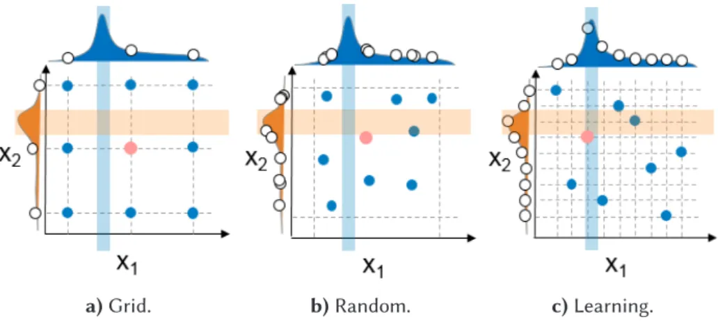
a)Grid. b)Random. c)Learning. Figure 2.6Automated Parameter Tuning Approaches.

best found HPs are reported and later used to solve a new, unforeseen problem instance.

In this part of thesis we outline existing automated approaches for parameter tuning, illustrating them in Figure 2.61. In this example, the TS exposes two parameters:X₁andX₂. Each figure shows dependencies betweenX₁(horizontal axis) andX₂(vertical axis) values and the subject of optimization along those axes (here the maximization case is depicted). The best configurations found by each approach are highlighted in pink.

Grid search parameter tuning. It is a rather simple approach for searching parameters. Here, the original search problem is relaxed and later solved by a brute-force algorithm. The set of all possible configurations (parameter sets) for relaxed problem is derived by specifying a finite number of possible values for each hyper-parameter under consideration. After evaluating all configurations on TS, the best-found solution is reported. Hence, this approach could skip promising parts of search space (Figure 2.6a). Moreover, the required time to probe all possible combinations is increasing by means of a factorial complexity.

Random search parameter tuning. This methodology relies on a random (often uniform) sampling of hyper-parameters and their evaluation on each iteration. At first sight, it might seem unreliable to chaotically traverse the search space. But empirical studies show that with a growing number of evaluations this technique starts to outperform grid search [9]. As an example, let us draw your attention to the best configurations (highlighted in pink) found by grid (Figure 2.6a) and random search (Figure 2.6b) techniques. The best randomly sampled configuration is definitely better than the one found by the grid search.

Heuristic search parameter tuning. By their nature, heuristic algorithms may be applied to tackle the most black-box search problems. Since the parameter tuning is one concrete type of search problem, it is also often tackled by a high-order heuristic approaches (meta-, hybrid-, hyper-heuristics) [25, 29, 30]. The advantage of heuristics usage lays in their ability to learn during the optimization process and use an obtained memory to guide the search more efficiently.

Model-Based Search Parameter Tuning. In most cases, the dependencies between tuned parameter values and optimization objective do exist and can be utilized for hyper-parameter tuning. By predicting

1