University of Louisville
ThinkIR: The University of Louisville's Institutional Repository
Electronic Theses and Dissertations5-2016
Computation of Least Angle Regression coefficient
profiles and LASSO estimates.
Sandamala Hettigoda
University of LouisvilleFollow this and additional works at:https://ir.library.louisville.edu/etd
Part of thePhysical Sciences and Mathematics Commons
This Master's Thesis is brought to you for free and open access by ThinkIR: The University of Louisville's Institutional Repository. It has been accepted for inclusion in Electronic Theses and Dissertations by an authorized administrator of ThinkIR: The University of Louisville's Institutional Repository. This title appears here courtesy of the author, who has retained all other copyrights. For more information, please [email protected].
Recommended Citation
Hettigoda, Sandamala, "Computation of Least Angle Regression coefficient profiles and LASSO estimates." (2016).Electronic Theses and Dissertations.Paper 2404.
COMPUTATION OF LEAST ANGLE REGRESSION COEFFICIENT PROFILES AND LASSO ESTIMATES
By
Sandamala Hettigoda
B.Sc., University of Kelaniya, Sri Lanka
A Thesis
Submitted to the Faculty of the
College of Arts and Sciences of the University of Louisville in Partial Fulfillment of the Requirements
for the Degree of
Master of Arts in Mathematics
Department of Mathematics University of Louisville
Louisville, KY
COMPUTATION OF LEAST ANGLE REGRESSION COEFFICIENT PROFILES AND LASSO ESTIMATES
Submitted by Sandamala Hettigoda
A Thesis Approved on
April 11, 2016
by the Following Examination Committee:
Professor Ryan Gill, Thesis Director
Professor Jiaxu Li
DEDICATION
ACKNOWLEDGEMENTS
No doubt first and foremost my deepest gratitude is to my adviser, Professor Ryan Gill one of the best teacher that I have had in my life. I am indebted to him for his encouragement, guidance and specially endless patience through out this project. How I forget his supportive and flexibility which help me not to bother at all continuing this thesis.
I would like to thank Professor Jiaxu Li and Professor K. B. Kulasekera, my committee members spending their valuable time and their highly motivated comments.
I would like to thank Professor Gamini Sumanasekara and family who put the foundation to start my higher studies in USA.
I like to express my gratitude to my dear friends Allan, Apsara, Bakeerathan, Chanchala and Udika who support me in numerous ways.
Finally I would like to thank to my family in Sri Lanka specially my eldest brother Nandana Hettigoda, my beloved husband Sujeewa, ever loving daughter Viyathma and son Vethum.
ABSTRACT
COMPUTATION OF LEAST ANGLE REGRESSION COEFFICIENT PROFILES AND LASSO ESTIMATES
Sandamala Hettigoda May 14, 2016
Variable selection plays a significant role in statistics. There are many vari-able selection methods. Forward stagewise regression takes a different approach
among those. In this thesis Least Angle Regression (LAR) is discussed in detail.
This approach has similar principles as forward stagewise regression but does not suffer from its computational difficulties. By using a small artificial data set and the well-known Longley data set, the LAR algorithm is illustrated in detail and the coefficient profiles are obtained. Furthermore a penalized approach to variable reduction called the LASSO is discussed, and it is shown how to compute its coeffi-cient profiles efficoeffi-ciently using the LAR algorithm with a small modification. Finally, a method calledK-fold cross validation used to select the constraint parameter for the LASSO is presented and illustrated with the Longley data.
TABLE OF CONTENTS
CHAPTER
1. INTRODUCTION . . . 1
2. LEAST ANGLE REGRESSION . . . 6
2.1 LAR Algorithm . . . 7
2.2 Example . . . 10
2.3 Code . . . 18
2.4 Longley Example . . . 21
3. PENALIZED REGRESSION VIA THE LASSO . . . 24
3.1 LASSO Algorithm via LAR Modification . . . 26
3.2 Code . . . 28
3.3 Longley Example . . . 30
4. SELECTION OF CONSTRAINT FOR THE LASSO . . . 34
4.1 Description of K-Fold Cross-Validation for the LASSO . . . 35
4.2 Longley Example . . . 36
5. CONCLUSION . . . 38
REFERENCES . . . 39
LIST OF TABLES
Table 2.1. Summary of the algorithm to obtain the coefficient profiles based
on the LAR method. . . 11
Table 2.2. LAR coefficient table for the standardized Longley data. . . 22
Table 2.3. LAR coefficient table for the Longley data (original scale). . . 23
Table 3.1. Modified LAR algorithm to obtain the coefficient profiles based
on the LASSO method. . . 27
Table 3.2. LASSO coefficient table for the standardized Longley data. . . 32
LIST OF FIGURES
Figure 2.1. Line segmentshx∗1,r˜∠1(α)i(red),±hx∗2,r˜∠1(α)i(green), andhx3∗,r˜∠1(α)i
(blue) for step 1 of the LAR algorithm. . . 13
Figure 2.2. Line segmentshx∗1,r˜∠2(α)i(red),hx∗2,r˜∠2(α)i(green), andhx3∗,r˜∠2(α)i
(blue) for step 2 of the LAR algorithm. . . 15
Figure 2.3. Line segmentshx∗1,r˜∠3(α)i(red),hx∗2,r˜∠3(α)i(green), andhx3∗,r˜∠3(α)i
(blue) for step 3 of the LAR algorithm. . . 17
Figure 2.4. Coefficient profiles for the artificial data example in Section 2.2. 18
Figure 2.5. LAR coefficient profiles for the standardized Longley data. . . 23
Figure 3.1. Contour plot ofkyc−X∗
β∗k2and LASSO constraintP2 j=1|β
∗
j| ≤
0.4 for the artificial example withX∗ = [x∗1 x∗2]. . . 25
Figure 3.2. LASSO coefficient profiles for the standardized Longley data. . 31
CHAPTER 1 INTRODUCTION
Linear regression is a method of fitting straight lines in accordance to the patterns of data, and it is one of the most widely used of all statistical techniques to analyze data. Simple linear regression is used to explain the relationship
be-tween a dependent variable (y) and an independent variable (x). The model with
an intercept is represented byy =β0 +β1x+, where is a error term with mean
0 and the variance is assumed to be a constant σ2. Given observed data points
(x1, y1), . . . ,(xn, yn), the simple linear regression model for the ith dependent
vari-able isyi =β0+β1xi+i where1, . . . , nare independent and identically distributed
random variables with variance σ2. In some cases, it is preferable to use a model
where the dependent variable is centered and the independent variable is rescaled; i.e., we define x∗i = xi−¯x
sx and y
c
i = yi−y¯ where ¯x = n1Pni=1xi and ¯y = n1Pni=1yi
are the sample means andsx =
q
1
n−1
Pn
i=1(xi−x¯)2 is the sample variance of thex
variable. With the centered data representation, the simple linear regression model can be expressed as
yic=β1∗x∗i +i. (1.1)
Note thatβ1 =β1∗/sx and β0 = ¯y−β1∗x/s¯ x= ¯y−β1x¯.
The best fit line ˆy = ˆβ0 + ˆβ1x is found by minimizing the residual sum of
squared errors Pni=1r2i where ri = yi −yˆi represents the ith residual. The residual
sum of squares can be expressed as
The method of least squares chooses ˆβ1 = Pn i=1(xi−¯x)(yi−¯y) Pn i=1(xi−x¯)2 and ˆβ0 = ¯y− ˆ β1x¯ which
minimizes the RSS. In the scaled model (1.1), the estimate is ˆβ1∗ =sxβˆ1.The sample
correlation is defined by Cor(x,y) = Pn i=1(xi−x¯)(yi−y¯) pPn i=1(xi −x¯)2 pPn i=1(yi−y¯)2
which is important in prediction. An alternate formula for the slope estimate in simple linear regression is
ˆ
β1 = Cor(x,y)
sy
sx
which shows the relationship between ˆβ1 and the sample correlation.
When there are p distinct predictors then the multiple linear regression
model is y = β0 + β1x1 + β2x2 +· · · + βpxp + . Given observed data points
(x11, . . . , x1p, y1), . . . ,(xn1, . . . , xnp, yn), the simple linear regression model for the
ith dependent variable is yi = β0 +β1xi1 +. . .+βpxip +i where 1, . . . , n are
independent and identically distributed random variables with variance σ2.
Simi-lar to simple linear regression, least squares estimation chooses ˆβ0,βˆ1, . . . ,βˆp which
minimizes RSS = n X i=1 (yi−β0−β1xi1−. . .−βpxip) 2 .
In matrix form, the goal is to estimate
β = β0 β1 .. . βp .
and the least squares estimate can be expressed as ˆβ= (X>X)−1X>
y whereX is
n×(p+ 1) matrix with columns
J = 1 .. . 1 ,x1 = x11 .. . xn1 , . . . ,xp = x1p .. . xnp , and y= y1 .. . yn .
Often, each of the ppredictor variables are scaled using the formulas
x∗ij = xij−x¯j
sj
and the response variable is centered using the formula
yci =yi−y¯
where ¯xj =
Pn i=1xij
n is the sample mean for the jth variable, and
sj = q
1
n−1
Pn
i=1(xij −x¯j)2 is the sample standard deviation for the jth variable.
Letting x∗1 = x∗11 .. . x∗n1 , . . . ,x∗p = x∗1p .. . x∗np , and yc= yc 1 .. . yc n ,
the least squares estimate for the centered model is given by ˆ
β∗ = (X∗>X∗)−1X∗>yc.
Especially when there are a large number of predictor variables available in the multiple linear regression model, it is desirable to consider strategies for selectively including variables in the model. Using too many predictor variables can lead to overfitting and standard error estimates for the coefficients can become inflated as discussed in Chapter 4 of Hocking (2013). Of course, if the number of predictor variables is greater than the number of observations, it is not even possible to include all of the predictor variables since (X>X)−1 does not exist if p≥n.
Different types of variable selection methods exist for regression models in statistics. The goal of each method is to identify the best subset among many variables to include in a model. Here are some basic strategies that can be used
for variable selection. Forward selection starts with a null model (no predictors
and only an intercept) and then proceeds to add one variable at a time according to the correlation until no additional variable is significant. Backward elimination
starts with the full model and deletes one variable at a time until all remaining variables are significant. Stepwise regression is a combination of forward selection and backward elimination methods. This method requires two significance levels. After each step, the significance level is checked, and it is determined whether a
variable should be added to or removed from the model. All subsets regression
builds all 2p possible models (including a model with only the intercept, all one
variable models, all two variables models, and so on).
Forward stagewise regression takes a different approach. It starts like for-ward selection with no variables included (usually the predictors are scaled and the responses are centered so this corresponds to a model with only an intercept) by setting the estimates for all coefficients equal to 0. Then the current residuals ri
are equal to the centered values yic, and the predictor xj most correlated with r
is selected. However, instead of fully adding the predictor x∗j to the model, the
coefficient estimate forβj is only incremented by a small amount ε·signhr,x∗jiand
the residuals are updated. This step is repeated many times until the remaining residuals are uncorrelated with each of the predictors. More discussion on forward selection, backward elimination, forward stagewise, all subsets, and forward stage-wise regression is given in Hastie, Tibshirani, and Friedman (2013).
If the value of ε used in forward stagewise regression is small, the coefficient estimates are updated very slowly from step to step and the number of steps re-quired to complete the algorithm can be very large. In this thesis, a closely related
method calledleast angle regression (LAR) which is motivated by the same
princi-ples but more computationally efficient will be discussed in detail. The algorithm
presented here is equivalent to that developed and described in Efron et al. (2004)
and Hastie, Tibshirani, and Friedman (2013). However, the notation used herein differs significantly from those classic references, and the paths for the coefficient profiles are parametrized differently.
In Chapter 2, the LAR algorithm is presented in detail, custom R code is provided implementing the presented version of the algorithm, and the method is illustrated using a small artificial data example as well as the well-known Long-ley data set. In Chapter 3, a penalized approach to variable reduction called the
LASSO is discussed and a method for computing the LASSO estimates using a modification of the LAR algorithm is presented and illustrated using the Longley data set. Finally, in Chapter 4, a method calledk-fold cross validation for choosing a model along the coefficient path for the LAR or LASSO algorithm is described and illustrated with the Longley data set.
CHAPTER 2
LEAST ANGLE REGRESSION
Just as in forward stagewise regression, the idea behind least angle regression is to move the coefficient estimates in the direction in which the predictor variable(s) is most correlated with the remaining residual. Instead of moving in steps of size
ε, the coefficient path for LAR changes continuously as it moves from a vector of
zeros to the least squares solution.
Finding the variable that is most highly correlated (in absolute terms) with the current residual is equivalent to finding the vector(s)x∗j which makes the
small-est angle with the residual r. The angle θ between two vectors x∗j and r can be
determined by cos(θ) = hx ∗ j,ri kx∗jkkrk = hx ∗ j,ri krk (since kx ∗ jk= 1) (2.1) = Cor(x∗j,r).
Thus, the absolute correlation|Cor(x∗j,r)|is maximized when|cos(θ)|is maximized
and consequently when the the absolute value of the angle, |θ|, is minimized. It
can be seen that the variable(s) which maximize (2.1) can be found by maximizing
hx∗j,risince krk does not depend on the index j.
A basic description of the LAR algorithm is as follows, similar to the algo-rithm provided in Algoalgo-rithm 3.2 on page 74 of Hastie, Tibshirani, and Friedman (2013).
1. Standardized the predictors to have mean zero and unit norm. Start with all estimates of the coefficients β1∗, β2∗, . . . , βp∗ to be equal to 0 with the residual
r∠
0 =yc.
2. Find the predictor xˆj∠
1 most correlated with the response r
∠
0.
3. Move the estimate of βˆj∗∠
1
from 0 towards the least squares coefficients until some other predictor xˆj∠
2 has as large a correlation with the current residual
˜
r1(α) as xˆj∠
1 does.
4. At this point instead of continuing in the direction based onxj1, LAR proceeds in a direction of equiangularity between the two predictors xˆj∠
1 and xˆj∠2. A
third variable xˆj∠
3 eventually earns its way into the most correlated (active
set), and then LAR proceeds equiangularly between xˆj∠
1,xˆj2∠, and xˆj∠3.
5. Continue adding variables to the active set in this way moving in the direction defined by least angle direction. Afteristeps this process gives a linear model with predictorsxˆj∠
1,xˆj∠2,xˆj3∠, . . . ,xˆji∠. After min(n−1, p) steps, the full least squares solution is attained and the LAR algorithm is complete.
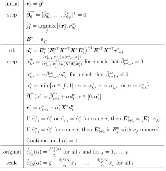
2.1 LAR Algorithm
In this section, the mathematical details of the LAR algorithm are developed in detail. This presentation of the LAR algorithm uses matrices which explicitly describe the coefficient directions on the ith step in terms of X∗ and r∠i−1 instead of using the active set terminology described in the classic references Hastie,
Tib-shirani, and Friedman (2013) and Efron et al. (2004).
On the initial step, let r∠0 =yc and ˆβ∗0∠ = [ ˆβ0∗,∠1, . . . ,βˆ0∗,p∠]> =0. Then choose the first variable that enters the model using the formula
ˆ j1∠= argmax j hx∗j,r∠0i .
Here is the algorithm for the ith step wherei= 1, . . . ,min{p, n−1}. Letej
be thejth standard unit vector inRp; for example,e
1 = [1,0, . . . ,0]>. The direction
on the ith step isd∠i =E∠i E∠i>X∗>X∗E∠i−1E∠i>X∗>r∠
i−1 whereE∠i is a matrix
with columns eˆj∠
1, . . . ,eˆj∠i. Then update the coefficient estimate using the formula ˜
βi∗∠(α) = ˆβi∗−∠1+αd∠i whereα is a value between [0,1] which represents how far the
estimate of β moves in the direction d∠i before another variable enters the model
and the direction changes again. We chooseαon theith step by finding the smallest value ofαsuch that the angle between the remaining residual ˜r∠i(α) = r∠i−1−αX∗d∠i
and one of the variables not in the model on the ith step (that is, a variable such that ˆβi∗−∠1,j = 0) equals the angle between ˜r∠i(α) and a variable in the model.
Mathematically, we choose α as follows. The angle between ˜r∠i (α) and the
jth variable x∗j equals the angle between ˜ri∠(α) and x∗ˆj∠ i
when
h˜r∠i(α),x∗ji=h˜r∠i(α),xˆ∗j∠
ii. (2.2)
Since it follows that
h˜r∠i(α),x∗ji = hr∠i−1−αX∗d∠i ,x∗ji
= hr∠i−1,x∗ji −αhX∗d∠i,x∗ji
= hr∠i−1,x∗ji −αhH∠ir∠i−1,x∗ji
= hr∠i−1,x∗ji −αhr∠i−1,H∠ix∗ji
whereH∠i =Zi(ZTiZi)−1ZTi is a hat matrix for Zi =X
∗ E∠i, the solution to (2.2) is ˜ αi,j+ = hr∠ i−1,x ∗ ˆj∠ i i − hr∠ i−1,x ∗ ji hr∠ i−1,H∠ixˆ∗j∠ i i − hr∠ i−1,H∠ix∗ji = hr∠i−1,x∗ˆj∠ i i − hr∠i−1,x∗ji hr∠ i−1,x ∗ ˆ j∠ i i − hr∠ i−1,H∠i x ∗ ji (2.3)
= hr∠i−1,x∗ˆj∠ i i − hr∠i−1,x∗ji hr∠ i−1,x ∗ ˆj∠ i i − hH∠i r∠ i−1,x ∗ ji = hr∠i−1,x∗ˆj∠ i i − hr∠i−1,x∗ji hr∠ i−1,x ∗ ˆj∠ i i − hX∗d∠i,x∗ji.
Equation (2.3) holds since Zi =H∠i Zi which implies that h xˆ∗j∠ 1 · · · x∗ˆj∠ i i =X∗E∠i =H∠i (X∗E∠i) = h H∠ix∗ˆj∠ 1 · · · H∠i xˆ∗j∠ i i so H∠i x∗ˆ j∠ k = x∗ˆ j∠ k
for k = 1, . . . , i. Similarly, the angle between ˜r∠i (α) and −x∗j
equals the angle between ˜r∠i(α) and x∗ˆ j∠ i when ˜ α−i,j = hr∠ i−1,x ∗ ˆ j∠ i i+hr∠ i−1,x ∗ ji hr∠ i−1,x∗ˆj∠ i i+hX∗d∠i,x∗ji.
So, the smallest value ofα such that a new variable should enter the model is
ˆ
α∠i = min
n
α∈[0,1] :α= ˜α+i,j or α= ˜α−i,j for some j such that ˆβi∗−∠1,j = 0 o . Then ˆβ∗i∠ = ˜β∗i∠( ˆα∠ i ), r∠i = yc−X ∗ˆ β∗i∠ = r∠ i−1−αˆ∠i X ∗
d∠i , and we move to the next step where ˆj∠
i+1 is the value of j such that ˜α +
i,j = ˆα∠i or ˜α
−
i,j = ˆα∠i .
So, the vector of LAR coefficient profiles based on the centered responses and standardized inputs can described by
ˆ β∗i∠(α) = 0 if i= 0 ˜ β∗1∠(α) if i= 1,0≤α≤αˆ∠1 .. . ... ˜
β∗min∠ {p,n−1}(α) if i= min{p, n−1},0≤α≤αˆmin∠ {p,n−1} and the vector of coefficient profiles based on the original scale is
ˆ β∠i (α) = h ˆ βi,∠0(α),βˆi,∠1(α), . . . ,βˆi,p∠(α) i> where ˆ βi,j∠(α) = ˆ β∗∠ i,j(α) sxj for j = 1, . . . , p
and ˆ βi,∠0(α) = ¯y− ˆ β∗∠ i,1(α) sx1 ¯ x1 −. . .− ˆ β∗∠ i,p(α) sxp ¯ xp.
A mathematical summary of the algorithm is given in Table 2.1.
2.2 Example
Here is a small artificial example to illustrate the LAR method. Suppose that we want to obtain the LAR coefficient profiles for
X = [x1 x2 x3] = 1 1 4 5 3 5 6 4 7 6 4 1 6 5 4 6 7 3 and y= 6 8 6 7 5 4 .
Then we standardize the inputs and center the outputs to obtain
X∗ = [x∗1 x∗2 x∗3] = −2 −1.5 0 0 −0.5 0.5 0.5 0 1.5 0.5 0 −1.5 0.5 0.5 0 0.5 1.5 −0.5 and yc= 0 2 0 1 −1 −2 . We initialize r∠ 0 =yc= [0,2,0,1,−1,−2] > and ˆβ∗∠ 0 = [0,0,0] >. Then we compute hx∗1,r∠ 0i=−1, hx ∗ 2,r∠0i=−4.5, and hx ∗ 3,r∠0i= 0.5 to determine that ˆj1∠= 2.
Consequently, on the first step, we have E∠1 =
0 1 0 and
initial r∠ 0 =yc step βˆ∗0∠ = [ ˆβ∗∠ 0,1, . . . ,βˆ ∗∠ 0,p] > =0 ˆ j1∠= argmax j hx∗j,r∠0i ith E∠i =heˆj∠ 1 · · · eˆj∠i i step d∠i =E∠i E∠i>X∗>X∗E∠i−1E∠i>X∗>r∠ i−1 ˜ α±i,j = hr∠ i−1,x∗ˆj∠ii∓hr ∠ i−1,x∗ji hr∠ i−1,x∗ˆj∠ i i∓hX∗d∠ i,x∗ji
for j such that ˆβi∗−∠1,j = 0
ˆ α∠ i = min α ∈[0,1] :α= ˜α+i,j or α= ˜α−i,j ˆ β∗i∠(α) = ˆβ∗i−∠1+αd∠i, α∈[0,αˆ∠ i] r∠ i =r∠i−1−αˆ∠iX ∗ d∠i ˆ j∠
i+1 is the value j such that ˜α + i,j = ˆα∠i or ˜α − i,j = ˆα∠i Continue until ˆα∠ i = 1. original βˆ∠ i,j(α) = ˆ β∗∠ i,j(α)
sj for all i and for j = 1, . . . , p
scale βˆ∠ i,0(α) = ¯y− ˆ β∗∠ i,1(α) s1 x¯1−. . .− ˆ β∗∠ i,p(α) sp x¯p for all i
Table 2.1 – Summary of the algorithm to obtain the coefficient profiles based on the LAR method.
d∠1 =E∠1 E1∠>X∗>X∗E∠1−1 E∠1>X∗>r∠ 0 = 0 −0.9 0 . Let ˜β∗1∠(α) = ˆβ0∗∠+αd∠1 = 0 −0.9α 0 and ˜ r∠1(α) =yc−X∗β˜1∗∠(α) = r∠0 −αX∗d∠1 = −1.35α 2−0.45α 0 1 −1 + 0.45α −2 + 1.35α
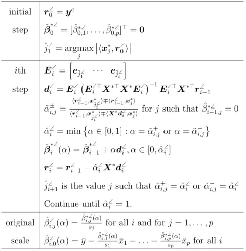
forα∈[0,1]. Then we compute±hx∗j,˜r∠1(α)iforj = 1,2,3 . We havehx∗1,r˜∠1(α)i=
−1 + 3.6α, hx∗2,r˜∠1(α)i = −4.5 + 4.5α, and hx∗3,˜r∠1(α)i = 0.5−0.9α. These line segments are plotted in Figure 2-1.
Then, we have hx∗1,r˜∠1( ˜α+11)i=hx∗2,r˜∠1( ˜α+11)i ⇒ α˜+11= −4.5 + 1 −4.5 + 3.6 = 35 9 ∈/ [0,1) h−x∗1,r˜∠1( ˜α11+)i=hx∗2,r˜∠1( ˜α+11)i ⇒ α˜−11= −4.5−1 −4.5−3.6 = 55 81 ≈.679 hx∗3,r˜∠1( ˜α+13)i=hx∗2,r˜∠1( ˜α+13)i ⇒ α˜+13= −4.5−0.5 −4.5−0.9 = 25 27 ≈.926 h−x∗3,r˜∠1( ˜α13−)i=hx∗2,r˜∠1( ˜α−13)i ⇒ α˜−13= −4.5 + 0.5 −4.5 + 0.9 = 10 9 ∈/ [0,1).
Figure 2.1 – Line segments hx∗1,˜r∠1(α)i (red),±hx∗2,r˜∠1(α)i (green), andhx∗3,r˜∠1(α)i
(blue) for step 1 of the LAR algorithm.
Thus, we have ˆα∠1 = 5581 so that ˆβ1∗∠ = ˜β∗1∠( ˆα1∠) =
0 −11 18 0 ≈ 0 −0.611 0 , r∠1 = ˜r∠1( ˆα∠1) = −11 12 61 36 0 1 −25 36 −13 12 ,
and ˆj∠
2 = 1.
Then, on the second step, we have E∠2 =
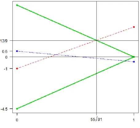
0 1 1 0 0 0 and d∠2 =E∠2 E∠2>X∗>X∗E∠2−1E∠2>X∗>r∠1 = 13 9 −13 9 0 . Let ˜β∗2∠(α) = ˆβ1∗∠+αd∠2 = 13 9 α −11 18 − 13 9α 0 and ˜ r∠2(α) =yc−X∗β˜2∗∠(α) = r∠1 −αX∗d∠2 = −11 12+ 13 18α 61 36− 13 18α −13 18α 1− 13 18α −25 36 −13 12+ 13 9α
forα∈[0,1]. Then we compute±hx∗j,˜r∠2(α)iforj = 1,2,3 . We havehx∗1,r˜∠2(α)i=
13 9 − 13 9α,hx ∗ 2,˜r∠2(α)i=− 13 9 + 13 9α, andhx ∗ 3,˜r∠2(α)i=− 1 9− 13
12α. These line segments
are plotted in Figure 2-2. Then, we have hx∗3,r˜∠2( ˜α23+)i=hx∗1,r˜∠2( ˜α+23)i ⇒ α˜+23= 13 9 − 1 9 13 9 + 13 12 = 48 91 ≈.527 h−x∗3,r˜∠2( ˜α23−)i=hx∗1,r˜∠2( ˜α−23)i ⇒ α˜−23= 13 9 + 1 9 13 9 − 13 12 = 56 13 ∈/ [0,1).
Figure 2.2 – Line segments hx∗1,r˜∠2(α)i (red), hx∗2,r˜∠2(α)i (green), and hx∗3,r˜∠2(α)i
(blue) for step 2 of the LAR algorithm.
Thus, we have ˆα∠2 = 4891 so that ˆβ2∗∠ = ˜β∗2∠( ˆα2∠) =
16 21 −173 126 0 ≈ 0.762 −1.373 0 , r∠2 = ˜r∠2( ˆα∠2) = −45 84 331 252 −8 21 13 21 −25 36 −9 28 ,
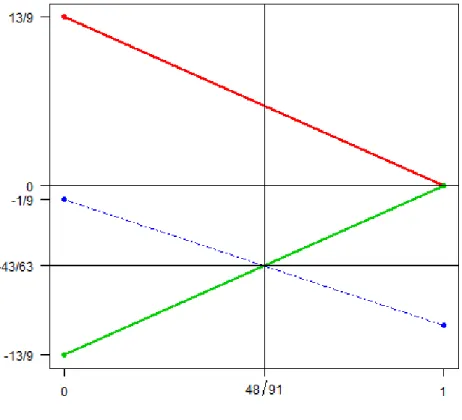
and ˆj∠ 3 = 3. Then E∠3 = 0 1 0 1 0 0 0 0 1 and d∠3 = E∠3 E3∠>X∗>X∗E∠3−1 E∠3>X∗>r∠ 2 = 10664 14007 −33497 42021 −172 667 . Let ˜β∗3∠(α) = ˆβ2∗∠+αd∠3 = 16 21 + 10664 14007α −173 126 − 33497 42021α −172 667α and ˜ r∠3(α) =yc−X∗β˜3∗∠(α) =r∠2 −αX∗d∠3 = −45 84+ 3053 9338α 331 252 − 22661 84042α −8 21 + 86 14007α 13 21 − 10750 14007α −25 36 + 215 12006α −9 28+ 6407 9338α
forα∈[0,1]. Then we compute±hx∗j,˜r∠3(α)iforj = 1,2,3 . We havehx∗1,r˜∠3(α)i=
−43 63+ 43 63α,hx ∗ 2,r˜∠3(α)i= 4363− 43 63α, and hx ∗ 3,˜r∠3(α)i= 4363− 43
63α. These line segments
are plotted in Figure 2-3. When α= 1, we get the least squares estimate
ˆ β∗3∠= 1016 667 −2895 1334 −172 667 ≈ 1.523 −2.170 −0.258 .
Since ¯y = 6, ¯x1 = 5, ¯x2 = 4, ¯x3 = 4 and sx1 = sx2 = sx3 = 2, the LAR
coefficient profiles are
ˆ βi,0(α) = 6 if i= 0 6 + 95α if i= 1,0≤α≤ 55 81 65 9 − 13 18α if i= 2,0≤α≤ 48 91 431 63 + 8686 42021α if i= 3,0≤α≤1 ,
Figure 2.3 – Line segments hx∗1,r˜∠3(α)i (red), hx∗2,r˜∠3(α)i (green), and hx∗3,r˜∠3(α)i
(blue) for step 3 of the LAR algorithm.
ˆ βi,1(α) = 0 if i≤1 13 18α if i= 2,0≤α ≤ 48 91 8 21+ 5332 14007α if i= 3,0≤α ≤1 , ˆ βi,2(α) = 0 if i= 0 −9 20α if i= 1,0≤α≤ 55 81 −11 36− 13 18α if i= 2,0≤α≤ 48 91 −173 252 − 33497 84042α if i= 3,0≤α≤1 , and ˆ βi,3(α) = 0 if i≤2 −86 667α if i= 3,0≤α≤1 .
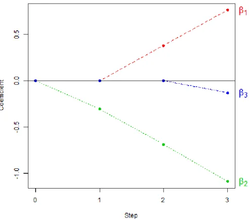
Figure 2.4 – Coefficient profiles for the artificial data example in Section 2.2. The LAR coefficient profiles for β1, β2, and β3 are illustrated in Figure 2.4.
2.3 Code
All of the computational work in the thesis was performed using the R sta-tistical software environment (R Core Team, 2015). The following custom function
our.larimplements the LAR algorithm as described in Section 2.1.
# LAR code from scratch
our.lar=function(X,y,epsilon=1e-8){ n=nrow(X)
p=ncol(X)
X.means=apply(X,2,mean) X.sds=apply(X,2,sd)
#center and scale the columns of X Xstar=X
for (i in 1:p)
Xstar[,i]=(X[,i]-X.means[i])/X.sds[i] #center the y variable
yc=y-mean(y)
#step up matrix to store the parameters that will be returned #from the function
beta.hat=rep(0,p+1) alpha.hat=NULL #initial step r=yc
#compute inner product and choose the first variable to enter #the model
inner.products=t(X)%*%r
j.hat=which.max(abs(inner.products)) #algorithm on the ith step
i=1 while ((i==1)||(alpha.hat[i-1]<1)){ beta.hat=rbind(beta.hat,rep(0,p+1)) alpha.hat=c(alpha.hat,1) njhat=length(j.hat) j.hat=c(j.hat,0) XE=Xstar[,j.hat] d=rep(0,p) d[j.hat]=solve(t(XE)%*%XE)%*%t(XE)%*%r Xd=Xstar%*%d #find alpha.hat[i] for (j in 1:p){ alpha=1 if (j%in%j.hat==FALSE){ if (abs(sum(Xstar[,j.hat[1]]*r)-sum(Xstar[,j]*Xd))>epsilon){ alpha=(sum(Xstar[,j.hat[1]]*r)-sum(Xstar[,j]*r))/ (sum(Xstar[,j.hat[1]]*r)-sum(Xstar[,j]*Xd)) if ((alpha<epsilon)|(alpha>1-epsilon)){ alpha=1
if (abs(sum(Xstar[,j.hat[1]]*r)+sum(Xstar[,j]*Xd))>epsilon){ alpha2=(sum(Xstar[,j.hat[1]]*r)+sum(Xstar[,j]*r))/ (sum(Xstar[,j.hat[1]]*r)+sum(Xstar[,j]*Xd)) if ((alpha2>epsilon)&(alpha2<1-epsilon)) alpha=alpha2 } } if (alpha+epsilon<alpha.hat[i]){ alpha.hat[i]=alpha j.hat[njhat+1]=j } } } } beta.hat[i+1,2:(p+1)]=beta.hat[i,2:(p+1)]+alpha.hat[i]*d r=r-alpha.hat[i]*Xd i=i+1 }
#translate coefficient estimates back to original scale beta.hat[,-1]=t(t(beta.hat[,-1])/X.sds)
beta.hat[,1]=mean(y)-beta.hat[,-1]%*%X.means #output relevant results
list(beta=beta.hat,alpha=alpha.hat) }
Here is code that can be used to compute the LAR coefficient profiles for the artificial data example in Section 2.2.
X=rbind( c(1,1,4), c(5,3,5), c(6,4,7), c(6,4,1), c(6,5,4), c(6,7,3)) y=c(6,8,6,7,5,4) print(our.lar(X,y)$beta,digits=4) print(our.lar(X,y)$alpha,digits=4)
> print(our.lar(X,y)$beta,digits=4) [,1] [,2] [,3] [,4] beta.hat 6.000 0.0000 0.0000 0.0000 7.222 0.0000 -0.3056 0.0000 6.841 0.3810 -0.6865 0.0000 7.048 0.7616 -1.0851 -0.1289
The rows give the values of ˆβ∠0, ˆβ∠1, ˆβ∠2, and ˆβ∠3, respectively. There is an excel-lent R package lars (Hastie and Efron, 2013) for implementing LAR, the LASSO, and forward stagewise regression. Using the package lars, the following command
coef(lars(X,y,type="lar")) verifies that the custom function above obtains the same coefficient profile as the classic LAR algorithm.
The other output commandprint(our.lar(X,y)$alpha,digits=4)
explic-itly computes the values of ˆα∠1, ˆα∠2, and ˆα∠3.
> print(our.lar(X,y)$alpha,digits=4) [1] 0.6790 0.5275 1.0000
2.4 Longley Example
As an example for Least Angle Regression consider the Longley data set which is studied extensively in Longley (1967). This data contained seven economi-cal variables observed annually from 1947 to 1960. There are 6 explanatory variables
x1, . . . , x6; they are the GNP implicit price deflator(GNP.deflator), Gross National
Product(GNP), number of people unemployed(Unemployed), number of people in the
armed force(Armed Force), non institutionalized population greater than 14 years
of age(Population), and the time(Year), respectively. The dependent variable yis
the number of people employed(Employed). The data set is also available in the R
data frame longley. The scale for the variables in R’s built-in data set is different from the scale in the original paper by Longley (1967); herein, the scale in the R data set is used.
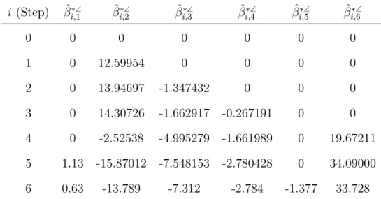
i (Step) βˆ∗∠ i,1 βˆ ∗∠ i,2 βˆ ∗∠ i,3 βˆ ∗∠ i,4 βˆ ∗∠ i,5 βˆ ∗∠ i,6 0 0 0 0 0 0 0 1 0 12.59954 0 0 0 0 2 0 13.94697 -1.347432 0 0 0 3 0 14.30726 -1.662917 -0.267191 0 0 4 0 -2.52538 -4.995279 -1.661989 0 19.67211 5 1.13 -15.87012 -7.548153 -2.780428 0 34.09000 6 0.63 -13.789 -7.312 -2.784 -1.377 33.728
Table 2.2 – LAR coefficient table for the standardized Longley data.
Coefficient tables obtained from the custom R function our.lar are given
in Table 2.2 (for the standardized predictors and centered response) and in
Ta-ble 2.3 for the variaTa-bles all in the original scale. It is seen that GNP is most
highly correlated with Employed since it is the first variable to enter the model.
Then Unemployed enters the model next, followed by Armed Force, Year, and
GNP.deflator. Population enters the model last and finally the least squares solution
ˆ
y=−13.789x2−7.312x3−2.784x4+ 33.728x6 + 0.63x1−1.377x5
is attained.
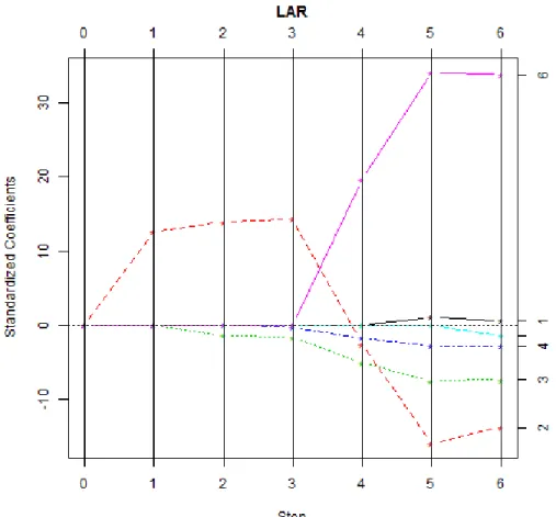
Figure 2.1 clearly shows the LAR coefficient profiles for the standardized
Figure 2.5 – LAR coefficient profiles for the standardized Longley data. i (Step) βˆi,∠0 βˆi,∠1 βˆi,∠2 βˆi,∠3 βˆi,∠4 βˆi,∠5 βˆi,∠6 0 65.32 0 0 0 0 0 0 1 52.63 0 0.03273 0 0 0 0 2 52.46 0 0.03623 -0.003723 0 0 0 3 52.63 0 0.03717 -0.004595 -0.0009913 0 0 4 -2011.32 0 -0.00656 -0.013802 -0.0061663 0 1.067 5 -3525.56 0.02701 -0.04123 -0.020856 -0.0103159 0 1.849 6 -3482.26 0.01506 -0.03582 -0.020202 -0.0103323 -0.0511 1.829
CHAPTER 3
PENALIZED REGRESSION VIA THE LASSO
Penalized regression methods estimate the regression coefficients by minimiz-ing the Residual Sum of Squares(RSS) which is based on Ordinary Least Squares(OLS) as in LAR. However penalized regression methods use a penalty on the size of the
regression coefficients. This penalty causes the regression coefficients to shrink
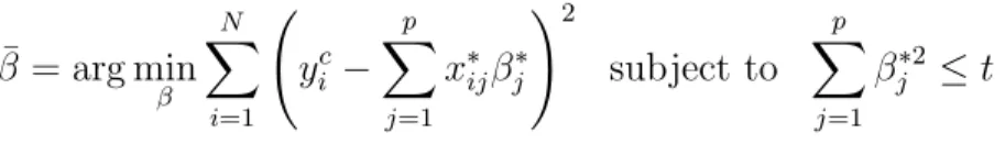
towards zero. Penalized regression methods include sequence of models each asso-ciated with specific values for one or more tuning parameters. Some versions of penalized regression keep all the predictors in the model; for example, ridge regres-sion coefficients minimize the RSS
¯ β = arg min β N X i=1 yic− p X j=1 x∗ijβj∗ !2 subject to p X j=1 βj∗2 ≤t
for some non-negative real number t.
Another method for penalized regression is the Least Absolute Shrinkage and Selection Operator(LASSO). The LASSO is a constrained version of OLS which minimizes the RSS subject to a constraint on the sum of absolute value of the regression coefficients. There is an important difference in LASSO with Ridge Re-gression. In Ridge Regression the L2 ridge penalty,
Pp j=1β ∗2 j is replaced by the L1 LASSO penalty,Ppj=1βj∗
. So the LASSO constraint makes the solutions non
lin-ear. Makingtsufficiently small will cause some of the coefficients to be zero. Often, the coefficient profiles for the LASSO are written as functions of the standardized
tuning parameters= Pp t
j=1|βˆ
∗
j|
.
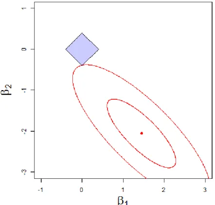
Figure 3.1 – Contour plot of kyc−X∗
β∗k2 and LASSO constraint P2
j=1|β
∗
j| ≤ 0.4
for the artificial example with X∗ = [x∗1 x∗2].
only x∗1 and x∗2 as explanatory variables with t = .4. The solid blue diamond
P2 j=1|β
∗
j| ≤ 0.4 gives the set of values of β
∗
1 and β
∗
2 which are permitted under
the LASSO constraint. The point at the center of the contour plot represents the least squares estimates ofβ1∗ and β2∗ based on the regression model of y onx∗1 and
x∗2. The red ellipses depicted in Figure 3.1 show level curves for the sum of squares functionkyc−X∗
β∗k2; the further the ellipse is from the center of the contour plot,
the larger the sum of squares function. Thus, it is seen from the contour plot that the constrained minimum of kyc−X∗β∗k2 is at the corner of the diamond where
β1∗ = 0. Hence, for t=.4, the first variablex∗1 is not included in the model.
simple modification of LAR algorithm gives a computationally efficient algorithm for computing the LASSO estimates. The main modification to the LAR algorithm is that if a non-zero coefficient hits zero, its variable must be dropped from the active set of variables and the current joint least squares direction should be recomputed. Thus, in the LASSO algorithm, variables can leave the model and possibly re-enter
later multiple times. Hence it may take more than p steps to reach the full model,
ifn−1> p, whereas in the LAR algorithm, variables added to the model are never removed, hence it will reach the full least squares solution using all variables in p
steps or less.
3.1 LASSO Algorithm via LAR Modification
The LAR algorithm with a minor modification provides an efficient algorithm
for computing the LASSO coefficient profiles. On the ith step, the modification
requires that none of the coefficient profiles cross 0. This is equivalent to considering other candidates for ˆα◦i that correspond to values of α such that ˆβ∗◦i−1 +αd◦i = 0. If ˆβi−1,j 6= 0, then let
˜
α∗i,j =−βˆi∗◦−1,j/d◦i,j.
Then,α is selected using the modified formula
ˆ
α◦i = min
n
α∈[0,1] :
α= ˜α+i,j or α= ˜αi,j− for some j such that ˆβi∗◦−1,j = 0
or
α= ˜α∗i,j for some j such that ˆβi∗◦−1,j 6= 0o.
Finally, the other modification is made if ˆα◦i = ˜α∗i,j for some j such that ˆβi∗◦−1,j 6= 0; in this case, E◦i is the matrix formed by removing the column ej from E◦i−1.
initial r◦0 =yc step βˆ∗◦0 = [ ˆβ0∗◦,1, . . . ,βˆ0∗◦,p]> =0 ˆ j1◦ = argmax j hx∗j,r◦0i E◦1 =eˆj◦ 1 ith d◦i =E◦i E◦>i X∗>X∗E◦i−1E◦>i X∗>r◦i−1 step α˜±i,j = hr◦i−1,x ∗ ˆj◦ i i∓hr◦i−1,x ∗ ji hr◦ i−1,x∗ˆji◦i∓hX ∗d◦
i,x∗ji for j such that ˆβ
∗◦
i−1,j = 0
˜
α∗i,j =−βˆi∗◦−1,j/d◦i,j for j such that ˆβi∗◦−1,j 6= 0 ˆ
α◦i = min
α∈[0,1] :α= ˜α+i,j, α = ˜α−i,j, or α= ˜α∗i,j
ˆ
β∗◦i (α) = ˆβ∗◦i−1+αd◦i, α∈[0,αˆ◦i]
r◦i =r◦i−1−αˆ◦iX∗d◦i
If ˜α+i,j = ˆα◦i or ˜α−i,j = ˆαi◦ for some j, then E◦i+1= [E◦i ej].
If ˜α∗i,j = ˆα◦i for some j, then E◦i+1 is E◦i with ej removed.
Continue until ˆα◦i = 1. original βˆi,j◦ (α) = βˆ
∗◦ i,j(α)
sj for all i and for j = 1, . . . , p scale βˆi,◦0(α) = ¯y−βˆ ∗◦ i,1(α) s1 x¯1−. . .− ˆ βi,p∗◦(α) sp x¯p for all i
Table 3.1 – Modified LAR algorithm to obtain the coefficient profiles based on the LASSO method.
3.2 Code
The following custom functionour.lassoimplements the LASSO algorithm
discussed in the previous section.
# LASSO code from scratch
our.lasso=function(X,y,epsilon=1e-8,max.steps=20){ n=nrow(X)
p=ncol(X)
#compute the mean and standard deviation of each column of X X.means=apply(X,2,mean)
X.sds=apply(X,2,sd)
#center and scale the columns of X Xstar=X
for (i in 1:p)
Xstar[,i]=(X[,i]-X.means[i])/X.sds[i] #center the y variable
yc=y-mean(y)
#step up matrix to store the parameters that will be returned #from the function
beta.hat=rep(0,p+1) alpha.hat=NULL #initial step r=yc
#compute inner product and choose the first variable to enter #the model
inner.products=t(X)%*%r
j.hat=which.max(abs(inner.products)) #algorithm on the ith step
i=1 while (((i==1)||(alpha.hat[i-1]<1))&(i<max.steps)){ beta.hat=rbind(beta.hat,rep(0,p+1)) alpha.hat=c(alpha.hat,1) njhat=length(j.hat) j.hat=c(j.hat,0) XE=Xstar[,j.hat] d=rep(0,p) d[j.hat]=solve(t(XE)%*%XE)%*%t(XE)%*%r Xd=Xstar%*%d #find alpha.hat[i] for (j in 1:p){ alpha=1 if (j%in%j.hat==FALSE){ if (abs(sum(Xstar[,j.hat[1]]*r)-sum(Xstar[,j]*Xd))>epsilon){ alpha=(sum(Xstar[,j.hat[1]]*r)-sum(Xstar[,j]*r))/ (sum(Xstar[,j.hat[1]]*r)-sum(Xstar[,j]*Xd)) if ((alpha<epsilon)|(alpha>1-epsilon)){ alpha=1 if (abs(sum(Xstar[,j.hat[1]]*r)+sum(Xstar[,j]*Xd))>epsilon){ alpha2=(sum(Xstar[,j.hat[1]]*r)+sum(Xstar[,j]*r))/ (sum(Xstar[,j.hat[1]]*r)+sum(Xstar[,j]*Xd)) if ((alpha2>0)&(alpha2<1)) alpha=alpha2 } } if (alpha+epsilon<alpha.hat[i]){ alpha.hat[i]=alpha j.hat[njhat+1]=j } } } else{ #LASSO modification if (d[j]!=0){ alpha=-beta.hat[i,j+1]/d[j] if ((alpha>0)&(alpha<alpha.hat[i])){ alpha.hat[i]=alpha j.hat[njhat+1]=-j } } } } if (j.hat[njhat+1]<0){
remove.j=-j.hat[njhat+1] j.hat=j.hat[abs(j.hat)!=remove.j] } beta.hat[i+1,2:(p+1)]=beta.hat[i,2:(p+1)]+alpha.hat[i]*d r=r-alpha.hat[i]*Xd i=i+1 }
#translate coefficient estimates back to original scale beta.hat[,-1]=t(t(beta.hat[,-1])/X.sds)
beta.hat[,1]=mean(y)-beta.hat[,-1]%*%X.means #output relevant results
list(beta=beta.hat,alpha=alpha.hat) }
The LASSO coefficient profiles and the α values can be extracted from the
output ofour.lasso the same way as the LAR coefficient profiles and theα values
were extracted from the output of our.lar.
3.3 Longley Example
Now, the LASSO method is illustrated on the Longley data set that was described in Section 2.4. The coefficient tables obtained from the custom R function
our.lasso are given in Table 3-2 (for the standardized predictors and centered response) and Table 3-3 for the variables all in the original scale.
Figure 3.1 clearly shows the LASSO coefficient profiles for the standardized Longley data. When using the LASSO, it is preferable to parameterize the coeffi-cient profiles by s instead of the index i for the step and the ˆα∠i that was used for the LAR algorithm.
The LASSO coefficient profiles are the same as the LAR coefficient profiles through step 3. On step 4, the LAR path for crosses 0. This is allowed for the LAR
algorithm, but it causes GNP to be dropped from the model when its path hits 0.
Figure 3.2 – LASSO coefficient profiles for the standardized Longley data.
direction for LAR. Eventually, at beginning of step 8,GNPre-enters the model, but
now with a negative coefficient. At the end of step 8, the path for GNP.deflator
hits 0, so it is dropped from the model; eventually it returns on the last step with the opposite sign for the coefficient.
i (Step) βˆi,∗◦1 βˆi,∗◦2 βˆi,∗◦3 βˆi,∗◦4 βˆi,∗◦5 βˆi,∗◦6 0 0 0 0 0 0 0 1 0 12.599536 0 0 0 0 2 0 13.946968 -1.347432 0 0 0 3 0 14.307258 -1.662917 -0.267191 0 0 4 0 0 -4.495328 -1.452729 0 16.72073 5 0 0 -5.109205 -1.921372 0 17.40197 6 0 0 -5.324667 -2.321762 -4.132012 21.83734 7 -0.3217731 0 -5.359592 -2.352200 -4.600470 22.65942 8 0 -4.664033 -6.019837 -2.498540 -3.510064 26.40331 9 0 -9.753905 -6.764499 -2.665480 -2.563231 31.09839 10 0.6295186 -13.788770 -7.311544 -2.784841 -1.376789 33.72789
i (Step) βˆi,◦0 βˆi,◦1 βˆi,◦2 βˆi,◦3 βˆi,◦4 βˆi,◦5 βˆi,◦6 0 65.32 0 0 0 0 0 0 1 52.63 0 0.03273 0 0 0 0 2 52.46 0 0.03623 -0.003723 0 0 0 3 52.63 0 0.03717 -0.004595 -0.0009913 0 0 4 -1701.67 0 0 -0.012421 -0.0053899 0 0.9068 5 -1772.89 0 0 -0.014117 -0.0071286 0 0.9438 6 -2224.44 0 0 -0.014712 -0.0086142 -0.15337 1.1843 7 -2308.69 -0.007699 0 -0.014809 -0.0087271 -0.17076 1.2289 8 -2705.65 0 -0.01212 -0.016633 -0.0092700 -0.13029 1.4319 9 -3201.50 0 -0.02534 -0.018691 -0.0098894 -0.09514 1.6865 10 -3482.26 0.015062 -0.03582 -0.020202 -0.0103323 -0.05110 1.8292
CHAPTER 4
SELECTION OF CONSTRAINT FOR THE LASSO
Selection of the constraint t in the LASSO plays an important role since it
controls the amount of regularization. One approach in such circumstances is to use a cross validation method to find the optimal value. Choosing the constraint depends on how many variables are included in the model, or equivalently how many coefficients are shrunk towards zero. Therefore each value corresponds to a model selection. There are a few kinds of cross validation methods (see, for instance, Chapter 7 of Hastie, Tibshirani, and Friedman (2013)). Herein a method called
K-fold cross validation is considered. In this method the data set is randomly
partitioned into K equal (or approximately equal) size parts. Then the method
leaves out one part as a test data set and fits the model based on the other K−1
parts combined together. The fitted model based onK−1 parts (the training data)
is used to obtain predictions for the left out part (test data), and the prediction error is recorded for each observation in the part that was left out. This process is
repeated using each of the K parts, and thus the prediction error is obtained for
all observations in the data set. Finally, there are different approaches for selecting the final model based on the average prediction error for each candidate model. While it is natural to choose the model which minimizes the average prediction error, some instead choose the model by visually identifying the “elbow” of the curve representing average prediction error as a function of the complexity of the model.
4.1 Description ofK-Fold Cross-Validation for the LASSO
First, the labels for the observations are randomly permuted to obtain a
design matrix ˘X and response vector ˘y. The rows of ˘X and ˘y are randomly
partitioned into K parts so that
˘ X = ˘ X1 ˘ X2 .. . ˘ XK and ˘y= ˘ y1 ˘ y2 .. . ˘ yK
where ˘Xk is an nk ×(p+ 1) matrix and ˘yk is a nk dimensional vector for k =
1, . . . , K. Usually,n1, . . . , nK are chosen to be approximately equal. Then, for each
k, the method proceeds to use the LASSO to estimate a coefficient profile denoted
by ˆβ◦−k(s) based on the design matrix ˘X(−k) =
˘ X1 .. . ˘ Xk−1 ˘ Xk+1 .. . ˘ XK
and response vector
˘ y(−k) = ˘ y1 .. . ˘ yk−1 ˘ yk+1 .. . ˘ yK
to predict ˘yk using the formula yb˘k = ˘Xkβˆ
◦
−k(s). The K-fold
cross-validation mean square error function for a LASSO model can be expressed as CV(s) = 1 n K X k=1 ky˘k−X˘kβˆ ◦ −k(s)k 2,
Figure 4.1 – 5-fold cross validation for the LASSO with the Longley data.
4.2 Longley Example
The built-in function cv.lars in the lars package can be used to obtain the cross-validation function. The following R commands can be used to compute the
function CV(s) withK = 5 and obtain the plot shown in Figure 4.1.
set.seed(32245)
cv.lasso.model=cv.lars(X,y,K=5,type="lasso",index=seq(0,1,by=.01))
In the above code, the random seed 32245 is useful to obtain reproducable
results based on the random partitioning of the observation into K = 5 parts.
The argument index=seq(0,1,by=.01)sets up a grid of values on whichCV(s) is
The minimum value s of the cross-validation function can be obtained with the following R commands.
w=which.min(cv.lasso.model$cv) s=cv.lasso.model$index[w] s
This code outputs the value s= 0.59, though if one wants to use the “elbow” estimate to obtain a result with lower complexity, a value near 0.2 should be used. Finally, the vector of coefficients can be obtained with the following R code.
lasso.model=lars(X,y,type="lasso") b=coef(lasso.model,s=s,mode="fraction") b
intercept=mean(y)-sum(apply(X,2,mean)*b) intercept
This code produces the fitted model
ˆ
CHAPTER 5 CONCLUSION
LASSO is a recently developed well-known variable selection method in statistics. It is a regression analysis method that performs at the same time both variable selection and regularization. The purpose of this thesis has been to study Least Angle Regression in full detail and subsequently study a computationally ef-ficient method for obtaining the LASSO coefef-ficient estimates. Rather than giving the brief compact version of the LAR algorithm, I described it with full mathemat-ical details which is easy to follow and understand. Furthermore, the algorithm is illustrated with the help of an artificial small example and a famous Longley data set including all necessary steps fully described.
With a small modification of the LAR algorithm, the LASSO is obtained and illustrated with the same two examples. Using my own R codes, both methods are implemented, and a comparison of the LAR and LASSO coefficient profiles are made with graphs and coefficient tables using the custom R code and the lars package.
To use the LASSO to estimate the regression coefficients, a point on the coefficient paths must be selected. That is, we must select a value for the penalty, or equivalently, the shrinkage factor. K-fold cross validation is a method which can
be used to accomplish this task, and an example of selcting the shrinkage factor s
REFERENCES
[1] Efron, B., Hastie, T., Johnstone, I., Tibshirani, R. (2004). Least angle regression.
The Annals of Statistics, 32, 407–499.
[2] Hastie, T. and Efron, B. (2013). lars: Least Angle Regression, Lasso and Forward Stagewise. R package version 1.2. https://CRAN.R-project.org/package=lars [3] Hastie, T., Tibshirani, R., and Friedman, J. (2013). The Elements of Statistical
Learning: Data Mining, Inference, and Prediction, second edition, 10th printing. Springer-Verlag.
[4] Hocking, R. R. (2013).Methods and Applications of Linear Models: Regression
and the Analysis of Variance, third edition. Hoboken, NJ: Wiley.
[5] Longley, J. W. (1967). An appraisal of least squares programs for the electronic computer from the point of view of the user.Journal of the American Statistical Association, 62, 819–841.
[6] R Core Team (2015). R: A language and environment for statistical computing. R Foundation for Statistical Computing, Vienna, Austria. URL https://www.R-project.org/
CURRICULUM VITAE Sandamala Hettigoda
Education
• B.Sc. in Physical Sciences, 1999, University of Kelaniya, Sri Lanka.
Teaching
• Graduate Teaching Assistant, Dept.of Mathematics, University of Louisville,
USA, Jan2016 - May2016
• Math Tutor, REACH, University of Louisville, USA, 2015 Aug -Jan 2016
• Mathematics Teacher, Carey College Colombo, Sri Lanka, 2000−2004
• Demonstrator, Dept. of Statistics and Computing, University of Kelaniya, Sri
Lanka, 1999−2000.
Certification
• Level I Tutor Training Certificate, REACH, University of Louisville, USA in
2015.
• Diploma in Computer Science, IDM, Sri Lanka in 1999
Research Experience