Bayesian Inference and Data Augmentation
Schemes for Spatial, Spatiotemporal and
Multivariate Log-Gaussian Cox Processes in
R
Benjamin M. Taylor Lancaster University Tilman M. Davies University of Otago Barry S. Rowlingson Lancaster University Peter J. Diggle Lancaster University Abstract
Log-Gaussian Cox processes are an important class of models for spatial and spa-tiotemporal point-pattern data. Delivering robust Bayesian inference for this class of models presents a substantial challenge, since Markov chain Monte Carlo (MCMC) algo-rithms require careful tuning in order to work well. To address this issue, we describe recent advances in MCMC methods for these models and their implementation in theR
package lgcp. Our suite of R functions provides an extensible framework for inferring covariate effects as well as the parameters of the latent field.
We also present methods for Bayesian inference in two further classes of model based on the log-Gaussian Cox process. The first of these concerns the case where we wish to fit a point process model to data consisting of event-counts aggregated to a set of spatial regions: we demonstrate how this can be achieved using data-augmentation. The second concerns Bayesian inference for a class of marked-point processes specified via a multivariate log-Gaussian Cox process model. For both of these extensions, we give details of their implementation inR.
Keywords: Cox process,R, spatiotemporal point process, multivariate spatial process, Bayesian
Inference, MCMC.
1. Introduction
A major goal of epidemiological research is to investigate the effects of environmental expo-sures on health outcomes. Our underlying premise is that cases of a health outcome arise in
a spatiotemporal continuum through the presence of a population at risk and a combination of environmental and individual characteristics that affect the risk of disease at each location in space and time. It is therefore natural to model both population density and risk as con-tinuous phenomena in time and space whilst recognising, firstly that the available data will be spatially incomplete and/or aggregated as well as susceptible to measurement error, and secondly that even after modelling the effects of all candidate variables, there will often be a residual component of spatiotemporal variation in risk that can only be captured by including in the model one or more latent, spatiotemporal stochastic processes.
In the present article, our focus is on Bayesian inference for a particular class of statistical models that in our opinion offer a flexible and intuitive framework for delivering answers to many scientific questions arising in spatial and spatiotemporal epidemiology: the log-Gaussian Cox process (LGCP). The spatial LGCP was introduced by Møller, Syversveen,
and Waagepetersen(1998). Brix and Diggle(2001) and Diggle, Rowlingson, and Su (2005a)
extended this class to include spatiotemporal processes. Diggle, Moraga, Rowlingson, and
Taylor(2013) discuss extensions of the LGCP methodology encompassing aggregated count
data and multivariate data. Open source software delivering the advanced Markov chain Monte Carlo (MCMC) methods required for inference has been a recent development in the form of the package lgcp (Taylor, Davies, Rowlingson, and Diggle 2013), but these meth-ods until now have been restricted to spatial and spatiotemporal LGCPs with known model
parameters.
When the goal of the analysis is spatial prediction, parameter uncertainty typically makes only a small contribution to the overall prediction error, and ad hoc methods of parameter estimation may suffice (Brix and Diggle 2001). However, in general it is more satisfactory to account for parameter uncertainty within a single analysis, and important to do so when pa-rameter values are of scientific interest in themselves, for example when estimating the effects of putative environmental exposures on the risk of disease. The Bayesian inferential frame-work provides an elegant and transparent means of encapsulating this uncertainty and also delivering joint inference on all model parameters including the latent field, the parameters of the latent field and covariate effects. The aim of this article is to present novel open-source software routines for Bayesian analysis of spatial, spatiotemporal, aggregated and multivari-ate LGCPs, delivering joint inference on all model parameters. For each of these classes, we provide a brief introduction to the statistical model and a walk-through analysis of a relevant dataset. The new methods are implemented in version 1.3 of the packagelgcp.
As in previous releases, the packagelgcpmakes extensive use of functions developed in theR
(R Core Team 2014) community. Specifically, many of the data structures are built around
pre-existing structures in the packages sp (Pebesma and Bivand 2005; Bivand, Pebesma,
and G´omez-Rubio 2013); spatstat (Baddeley and Turner 2005); RandomFields (Schlather,
Malinowski, Menck, Oesting, and Strokorb 2015); andncdf(Pierce 2014). New and significant
dependencies include the packagesrgeos(Bivand and Rundel 2013) andraster (Hijmans and
van Etten 2013).
To our knowledge, the packagelgcpis unique as anRpackage specifically designed for MCMC-based Bayesian inference for log-Gaussian Cox Processes. Approximate Bayesian inference for log-Gaussian Cox processes may also be performed using the popularINLApackage (Rue,
Martino, and Chopin 2009; Lindgren, Rue, and Lindstr¨om 2011). The package INLA can
be used for the modelling of general latent Gaussian processes and the integrated nested Laplace approximation (INLA) methodology has been used for inference with log-Gaussian
the author introducesRpackagesgeostatspandgeostatsinlato make the interface to functions from theINLA package more user-friendly and furthermore provides an example in which a spatial log-Gaussian Cox process is used to model incidences of murder in Toronto.
The main advantage of using integrated nested Laplace approximations for inference with log-Gaussian Cox processes is computational cost, although this issue is not completely clear-cut, see for example Taylor and Diggle (2014). When using the package INLA, invoking strategy = simplified.laplace in the control.inla argument list, delivers the fastest, but least accurate inference. One advantage of the MCMC-based implementation provided in the packagelgcpoverINLA-based counterparts is that once stationarity has been reached, MCMC produces unbiased samples from the joint posterior of all model parameters. The MCMC methods in the package lgcp furthermore permit the use of any valid covariance function, rather than being restricted to a subset of the Mat´ern class.
As pointed out inTaylor and Diggle (2014), we believe that both INLA and MCMC are im-portant inferential tools in the analysis of spatial and spatiotemporal data. INLA is especially convenient for model selection, but once this has been reduced to a single model, a long run of a carefully designed MCMC algorithm may be a safer option for performing inference. Lastly, the two approaches are not mutually exclusive: inHaran and Tierney(2012), the authors use a heavy tailed approximation similar to INLA to construct efficient MCMC proposal schemes. The remainder of this article is structured as follows. In Section 2, we introduce the log-Gaussian Cox process. In Section 3, we provide a brief introduction to Bayesian inference and MCMC for LGCPs. In Section4, we introduce four LGCP models and for each example, provide a practical R session to be used as guidance on the implemention of our MCMC routines, diagnostics and post-processing. Specifically, in Section4.1we discuss the Bayesian analysis of spatial point process data; in Section 4.2 we analyse a dataset consisting of case counts aggregated to regions; in Section4.3we perform a Bayesian analysis of a spatiotemporal LGCP; and in Section 4.4 we analyse a multivariate LGCP. The article concludes with a discussion in Section5.
2. The log-Gaussian Cox process
In this section, we introduce the log-Gaussian Cox process; for simplicity, we focus the dis-cussion on spatial LGCPs. Throughout this article, we let X be the observed data, Z be measured covariates, β be the effect size and Y be the residual process; also let π denote a generic probability density function.
We begin with some definitions. An intensity process, R : S → [0,∞), is a non-negative valued stochastic process: a function from a non-null measurable set, in this case S ⊂ R2,
to the non-negative real line, [0,∞). A locally finite random set X ⊂S is known as a Cox
process directed by an intensity process, R, if the conditional distribution ofX given R is a
Poisson process with intensityR. This means that for any bounded Borel setB, card(X∩S)∼Poisson Z B R(s)ds .
If{Y(s) :s∈R2}is a spatial stochastic process with the property that for any finite collection,
thatY is aGaussian process. Alog-Gaussian Cox process is a Cox process whose log-intensity is a Gaussian process.
In the remainder of the article, we will assume that computation takes place on a regular fine grid. We think of s as belonging toR2, but use the notation X(s) to denote the number of events in the computational grid cell containing s. In this article, we therefore notate the spatial log-Gaussian Cox process as follows:
X(s) ∼ Poisson{R(s)}
R(s) = CAλ(s) exp{Z(s)β+Y(s)},
where CAis cell area, λ(s) is a known population offset,Z(s) is a vector of covariate values,
with associated effectsβ,Y is a Gaussian process; the notational extension to spatiotemporal and multivariate processes will be obvious. In practice, we aim to make the computational grid as fine as possible, ideally sufficiently fine that each cell count is either zero or one with high probability.
Our model for the covariance matrix of the process Y on the computational grid will come from a parametric family. Typically, these parameters include a variance parameter,σ2, and a scale parameter,φ. We setE[Y] =−σ2/2 which, using the properties of a log-Normal random variable, gives E[exp(Y)] = 1; this parametrisation also has an advantage in that exp(Y) can be interpreted as covariate-adjusted relative risk. We will use η to denote the parameters of the covariance function transformed onto an appropriate scale for the MCMC algorithm e.g., in this article we use η={log(σ),log(φ)}.
3. Inference for log-Gaussian Cox processes
In this section, we provide a brief review of two inferential techniques for LGCPs. In Section
3.1, we explain a computationally simple approach to parameter estimation for the parameters of the process Y, the minimum contrast estimator. Then in Section 3.2, we explain how Bayesian inference can be used to deliver inference for all model parameters: β,η and Y. 3.1. Minimum contrast parameter estimation
It is useful to have fast methods that provide provisional estimates of the parameters of the latent Gaussian process, Y. Such an estimate can be used to decide how fine the compu-tational grid must be in order to capture spatial dependence in Y. Møller et al. (1998) use the method ofminimum contrast estimation (also referred to as the least-squares approach). Minimum contrast methods involve finding the parameter values which minimise the squared discrepancy between the assumed parametric form of the second-order characteristic of in-terest (in our context this will represent either the spatial or temporal covariance), and a corresponding nonparametric estimate thereof. For a comprehensive overview of minimum contrast estimation for spatial and spatiotemporal LGCPs, including a suite of simulation studies gauging proximity of minimum contrast parameter estimates to their true values, see
Davies and Hazelton (2013).
The parametric functions typically used for spatial minimum contrast are the pair correlation function (PCF) g and Ripley’s K function (Ripley 1977). These are convenient because they are theoretically tractable within the LGCP framework, and they also have accessible
corresponding nonparametric estimate based on the observed data. The general form of the minimum contrast criterion with respect to spatial lags u is
MJ(σ2, φ) = Z umax u0 w(u)v{Jˆ(u)} −v{Jσ2,φ(u)} 2 du ≈u−diff1 X u∈U w(u) v{Jˆ(u)} −v{Jσ2,φ(u)} 2 , (1)
whereu0 is the smallest spatial lag to be considered (typically zero, though this must
tech-nically be > 0 for evaluation of the nonparametric PCF), umax is an upper bound on the
distances to be considered (typically chosen as some fraction the size of the spatial observa-tion window),w(u) represents an optional set of lag-dependent weights andv{ · }is an optional transformation to be applied to the quantities of interest. The integral is approximated in practice by summing over a fine, evenly spaced sequence of valuesU ={u0, u1, . . . , umax}such
that udiff is the difference between any two consecutive terms in U. It is worth noting that
dependent upon the design of the model under scrutiny, ˆJ may represent either the homoge-neous or inhomogehomoge-neous version of the nonparametric estimator, with the fixed heterogehomoge-neous intensity in the latter case specified by some external means.
A similar construction is used in Brix and Diggle (2001) and Diggle et al. (2005a) for esti-mation of the scale of temporal dependence (parameter θ). In that setting, the first step is to estimate the spatial parameters by Equation 1 using ‘time-averaged’ versions of K or g. Then, estimation ofθproceeds using the temporal autocorrelation function of the frequency of observations over time. The spatial parameter estimates are plugged-in to the theoretical formulation of the temporal correlation, expressions for which can be found inBrix and Diggle
(2001) (see also the corrections made inBrix and Diggle 2003;Taylor and Diggle 2013). Minimum contrast methods suffer from the somewhat arbitrary nature in which one must ‘cal-ibrate’ the criterion via e.g.,umax,w, andv, not to mention whether use ofg is ‘better’ than
K or vice versa in Equation 1. Use of g also requires selection of a smoothing bandwidth
for its nonparametric estimation. There have been some efforts in the literature to aid in these decisions, involving both theoretical e.g., (Guan and Sherman 2007) and numerical e.g.,
(Diggle and Ribeiro 2003) endeavours. Concerns over subjectiveness aside, Davies and
Tay-lor (2014) indicate minimum contrast methods perform well against approximate likelihood methods in terms of practical performance.
3.2. Bayesian inference and the role of MCMC
In this section we introduce Bayesian inference and, using the example of a spatial log-Gaussian Cox process as an illustration, explain the details of our new methods for the practical fitting of models from this class.
In a ‘Classical’ or ‘Frequentist’ analysis, statistical inference is usually concerned with making statements about the asymptotic distribution of the maximum likelihood estimates. When this maximisation problem is in some sense intractable, either because the likelihood is not analytic or because the optimisation problem is too hard, an alternative is to use Bayesian methods (Bernardo and Smith 2008).
likelihood), which determines the density π(X|β, η, Y); and 2) a set of prior beliefs about the distribution of the parameters, expressed through the probability densityπ(β, η, Y). By Bayes’ Theorem, the product of the prior and likelihood is proportional to the posterior:
π(β, η, Y|X) = π(X|β, η, Y)π(β, η, Y)
π(X) ∝π(X|β, η, Y)π(β, η, Y);
the quantityπ(X) is called the marginal likelihood. Note that the conditional independence properties of this model imply thatπ(X|β, η, Y) =π(X|β, Y).
Bayesian statistical inference is concerned with making probabilistic statements about the posterior, π(β, η, Y|X), however, in almost all non-trivial applications it is not possible to make analytic probability statements about this density function. In order to proceed, we therefore must resort to either 1) making statistical inference from an approximation of the posterior; or 2) sample-based Monte Carlo inference, based on a sample,{β(j), η(j), Y(j)}N
j=1,
drawn from π(β, η, Y|X). In this article, we refer to the former as ‘approximate meth-ods’ because inference is not based on the true posterior; and we refer to the latter as ‘exact’ methods because as N → ∞, any sample-based estimate of a posterior expecta-tion of interest, N1 PN
i=1f(β(j), η(j), Y(j)), is an unbiased estimator of the exact quantity,
Eπ(β,η,Y|X)[f(β, η, Y)], for any functionf where this expectation exists.
Some advantages of the Bayesian approach are: that it provides a transparent framework for inference; secondly, it is flexible and often provides an elegant and practical solution to inference arising from very complex statistical models. Note, in particular, that Bayesian methods make no formal distinction between estimation ofβ and η and prediction ofY, and in this way naturally incorporate parameter uncertainty into predictive inference. Against this, obtaining the sample {β(j), η(j), Y(j)}N
j=1∼π(β, η, Y|X) can itself be a major challenge.
Along with Gibbs sampling, the most commonly employed method for generating the sam-ple{β(j), η(j), Y(j)}N
j=1 is the Metropolis-Hastings algorithm (Metropolis, Rosenbluth,
Rosen-bluth, Teller, and Teller 1953;Hastings 1970). The idea is to simulate from a Markov chain
whose stationary distribution is the target of interest, namelyπ(β, η, Y|X). Having initialised the chain at time 0, {β(0), η(0), Y(0)}, theith step of the algorithm involves drawing a candi-date {β∗, η∗, Y∗}from a proposal density, q(β∗, η∗, Y∗|β(i−1), η(i−1), Y(i−1)) and accepting it, i.e., setting {β(i), η(i), Y(i)}={β∗, η∗, Y∗}, with probability
min ( 1, π(β ∗, η∗, Y∗|X) π(β(i−1), η(i−1), Y(i−1)|X) q(β(i−1), η(i−1), Y(i−1)|β∗, η∗, Y∗) q(β∗, η∗, Y∗|β(i−1), η(i−1), Y(i−1)) ) .
The design of q is critical and forms a major stem of academic research in this field, see
Gilks, Richardson, and Spiegelhalter (1995) and Gamerman and Lopes (2006) for reviews.
The design ofq in the package lgcp, discussed below, is a mix of random walk and Langevin proposal kernels. Whilst in some sense the random walk is a blind proposal mechanism, the main idea of using a Langevin kernel, known as the Metropolis-adjusted Langevin algorithm (MALA), is to exploit gradient information on the target to help propose moves towards areas of higher posterior probability. An alternative to the MALA for log-Gaussian Cox process is Hamiltonian Monte Carlo (Girolami and Calderhead 2011). Hamiltonian methods have better theoretical mixing properties compared with a MALA, but are more difficult to tune, requiring pilot runs of the algorithm (Neal 2011). It is for this reason that we have chosen to implement a MALA in the package lgcp: in practice we can adaptively choose a
As in previous implementations of a MALA for the LGCP, we work with a transform ofY, namely Γ, where Y = Σ1η/2Γ +µη and a subscript η denotes dependence on the parameters
of the latent process, η (Møller et al. 1998; Brix and Diggle 2001; Diggle et al. 2013). Let
ζ = {β, η,Γ}. A full Metropolis-adjusted Langevin algorithm for our target would use the following proposal kernel:
q(ζ(i∗)|ζ(i−1)) = N ζ(i∗);ζ(i−1)+h 2 2 Σopt∇log{π(ζ (i−1)|X)}, h2Σ opt , (2)
where h is a scaling constant. The ideal choice for Σopt would be the inverse of the Fisher
information matrix evaluated at the maximum likelihood estimate ofζ (Girolami and
Calder-head 2011). Unfortunately, due to the high dimensionality ofζ, it is infeasible to work with
this matrix. However, we are at liberty to use an approximation of the optimal choice and it transpires that in doing this we can still obtain an efficient algorithm.
As mentioned above, we use a proposal kernel that is a mix of random walk and MALA components. The proposal variance matrix is block diagonal, where each block is an approx-imation of the inverse of the Fisher information matrix. We mix random walk and MALA proposals because the gradient of the target with respect toηis in general difficult to compute and also computationally costly. We suggest the following overall proposal:
q(ζ(i∗)|ζ(i−1)) = Nhζ(i∗);µζ(i−1), h2Σ i . (3) where µζ(i−1) = Γ(i−1)+h 2h2 Γ 2 ΣΓ ∂log{π(ζ(i−1)|Y)} ∂Γ β(i−1)+h 2h2 β 2 Σβ ∂log{π(ζ(i−1)|Y)} ∂β η(i−1) and Σ = h2ΓΣΓ 0 0 0 h2 βΣβ 0 0 0 ch2ηΣη (4)
In Equation4, ΣΓis an approximation to the negative inverse of the Fisher information matrix,
{−E[I(ˆΓ)]}−1, and similarly for Σ
β and Ση. The constants h2Γ,h2β and h2η are approximately
optimal scalings for Gaussian targets explored by Gaussian random walk or MALA proposals,
seeRoberts and Rosenthal(2001). We set h2Γ= 1.652/dim(Γ)1/3,h2β = 1.652/dim(β)1/3 and
h2
η = 2.382/dim(η), where dim is the dimension. In the package lgcp, we construct ΣΓ, Σβ
and Ση based on initial ad hoc guesses at Γ,β and η followed by a quadratic approximation
to the target. We tune h so that the MCMC algorithm has an average acceptance rate of 0.574, which is approximately optimal for the MALA components. However, in order to have the random walk block running at approximate optimality, we introduce the scaling constant
c= 0.4 to temper the proposals in the ηcomponent; we have observed that this choice works well across a variety of scenarios.
The package lgcp allows the user to specify a prior of the form π(β, η,Γ) = π(β)π(η)π(Γ). FollowingMøller et al. (1998) and Brix and Diggle(2001), we set the prior for Γ to π(Γ) = N(0, I), where I is the identity matrix. This is a sensible prior for Γ, given the relationship withY, so we do not allow the user to modify this choice. The userishowever able to specify priors forβ and η, as will be demonstrated below. Although a prior of the formπ(Γ)π(β, η)
would give the user greater choice, in practical contexts it is difficult to justify an a priori
covariance structure betweenβ and η.
4. Worked examples
In this section, we provide four worked examples. Each of these examples assumes a different statistical model for the data: in Section 4.1, we use a spatial LGCP to model cases of primary biliary cirrhosis in Newcastle-Upon-Tyne; in Section 4.2, we re-visit the cirrhosis data, but pretend the case counts had been aggregated to regions; in Section 4.3, we use a spatiotemporal LGCP to model cases of gastrointestinal infection in Hampshire; lastly, in Section 4.4, we use a multivariate LGCP to investigate the spatial segregation of four genotypes of bovine tuberculosis in Cornwall.
Due to the computationally demanding nature of some aspects of the model fitting process, we recommend the user follows the procedure detailed in Algorithm1. Although pilot runs are not strictly necessary for implementing the adaptive MCMC algorithm, it is nevertheless wise to perform some short runs to make sure everything appears to be in order before committing a large chunk of computation time to a long MCMC run for the final analysis. We have found that printing the current value ofhto the console is invaluable as an online check in step5of Algorithm1; this is done in all our implementations below. The scaling parameterhtends to converge very quickly, so using this in pilot runs of 1,000–5,000 iterations as a guide to help choose the number of iterations for the final run is well worthwhile.
In our experience of using this MCMC algorithm, we have found that values of h between 0.5 and 1 usually indicate that the chain is mixing very well and 500,000–1,000,000 iterations is usually sufficient to achieve convergence; values between 0.2 and 0.5 will likely need to be run for slightly longer to achieve convergence e.g., 1,000,000–3,000,000 iterations; and values around 0.02–0.05 will likely need a considerable number of iterations to achieve stationarity e.g., 20,000,000 iterations.
4.1. PBC in Newcastle-Upon-Tyne, a spatial point process model
Introduction
In the next two sections we re-visit a point process dataset originally analysed in Prince,
Chetwynd, Diggle, Jarner, Metcalf, and James (2001). These data consist of geo-referenced
cases of definite or probable primary biliary cirrhosis (PBC) alive between 1987 and 1994. In this section, we treat these data as they were collected: as a spatial point process dataset. Our statistical model is given in Equation5:
X(s) = Poisson[R(s)], (5)
R(s) = CAλ(s) exp{Z(s)β+Y(s)}.
Here X(s) is the number of events in the cell of the computational grid containing s, R(s) is the Poisson rate,CA is the cell area, λ(s) is a known offset, Z(s) is a vector of measured
covariates and Y(s) is the latent Gaussian process on the computational grid. The other parameters in the model areβ, the covariate effects; andη ={log(σ),log(φ)}, the parameters of the processY on an appropriately transformed (in this case log) scale.
1: We recommend computing approximate values of the parameters, η, of the process Y
using ad hoc methods. These approximate values are used for two main reasons: (1) to help inform the size of the computational grid, since we will need to use a cell width that enables us to capture the dependence properties of Y and (2) to help inform the proposal kernel for the MCMC algorithm.
2: We recommend that the user choose an appropriate grid on which to perform inference; this will partly be determined by the results of the first stage and partly by the available computational resources available to perform inference.
3: If environmental covariates are used in the analysis, we suggest that the user next
constructs an overlay of these data (in the form of SpatialPixelsDataFrame or SpatialPolygonsDataFrame objects) onto the computational grid that will be used in the subsequent analysis. This can be an expensive step, aslgcpemploys polygon/polygon overlays to infer covariate values on the grid. We further recommend that the user saves this object after it has been constructed, and in future reference to the data reloads this object, rather than having to re-compute it.
4: Decide on which covariates are to play a part in the analysis and use the lgcp functions to interpolate these onto the computational grid. Note that having saved the results from step three, this is a relatively quick operation, and allows the user quickly to construct different design matrices, Z, from different candidate models for the data.
5: Set up the population offset and specify the priors and, if desired, the initial values for the MCMC.
5: Run the MCMC algorithm and save the output to disk. We recommend dumping infor-mation to disk because it offers much greater flexibility in terms of MCMC diagnosis and post-processing.
6: Perform post-processing analyses including MCMC diagnostic checks and produce sum-maries of the posterior expectations we require for presentation.
Analysis of a point-process dataset
We start by loading thelgcppackage and data for this example.
R> library("lgcp")
R> load("sd_liver.RData")
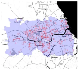
The point process data are contained in an objectsdofspatstatclassppp; these are a subset of the original data consisting of 415 cases located in the Newcastle-Upon-Tyne area, illustrated in Figure 1; the background of this figure was obtained using the OpenStreetMap package
(Fellows 2013).
Along with the case data, our covariate information consists of population counts and socio-demographic information in aSpatialPolygonsDataFrameobject.
R> load("popshape_liver.RData")
This loads an object calledpopshapeconsisting of population counts (total and male/female counts) and the 7 individual domains of the Index of Multiple Deprivation (IMD) measured
Figure 1: Plot of cases of primary biliary cirrhosis in Newcastle-Upon-Tyne.
at the Lower Super Output Area (LSOA) level. Since this is only an illustrative example of our methodology and Rcode, we used population data from the 2001 census and IMD data from the 2007 report. We constructed a variable propmaleequal to the proportion of males in each of the LSOAs.
We now have all the raw information required to fit the model in Equation 5 and begin, according to Algorithm1, by obtaining approximate estimates of the parameters.
R> minimum.contrast(sd, model = "exponential", method = "g", + intens = density(sd), transform = log)
$estimates scale variance [1,] 275.6771 1.560087 $discrepancy Squared discrepancy [1,] 299.1335
As the approximate spatial scale of dependence, 275 metres, is quite small, this tells us that quite a fine grid might be necessary to capture the dependence structure in the process Y. We use the commandchooseCellwidthinteractively to choose an appropriate grid size:
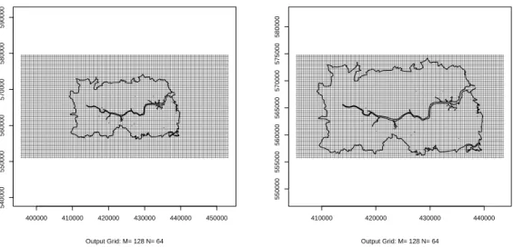
R> chooseCellwidth(sd, cwinit = 300)
Running this command several times with different values of cwinit produces plots of the computational grid overlaid on top of the observation window; the size of the output grid appears in the subtitle. Figure2 shows two such plots; note that computation grids of size 2m×2n for some positive integers m and n are the most efficient sizes for the Fast Fourier Transform (Wood and Chan 1994; Taylor and Diggle 2014). Both of the plots in this figure show output grids of size 128×64, but the right-hand plot, using a cellwidth of 300, is the
400000 410000 420000 430000 440000 450000 540000 550000 560000 570000 580000 ++++++++++++++++++++++++++++++++++++++++++++++++++++++++++++++++++++++++++++++++++++++++++++++++++++++++++++++++++++++++++++++++ ++++++++++++++++++++++++++++++++++++++++++++++++++++++++++++++++++++++++++++++++++++++++++++++++++++++++++++++++++++++++++++++++ ++++++++++++++++++++++++++++++++++++++++++++++++++++++++++++++++++++++++++++++++++++++++++++++++++++++++++++++++++++++++++++++++ ++++++++++++++++++++++++++++++++++++++++++++++++++++++++++++++++++++++++++++++++++++++++++++++++++++++++++++++++++++++++++++++++ ++++++++++++++++++++++++++++++++++++++++++++++++++++++++++++++++++++++++++++++++++++++++++++++++++++++++++++++++++++++++++++++++ ++++++++++++++++++++++++++++++++++++++++++++++++++++++++++++++++++++++++++++++++++++++++++++++++++++++++++++++++++++++++++++++++ ++++++++++++++++++++++++++++++++++++++++++++++++++++++++++++++++++++++++++++++++++++++++++++++++++++++++++++++++++++++++++++++++ ++++++++++++++++++++++++++++++++++++++++++++++++++++++++++++++++++++++++++++++++++++++++++++++++++++++++++++++++++++++++++++++++ ++++++++++++++++++++++++++++++++++++++++++++++++++++++++++++++++++++++++++++++++++++++++++++++++++++++++++++++++++++++++++++++++ ++++++++++++++++++++++++++++++++++++++++++++++++++++++++++++++++++++++++++++++++++++++++++++++++++++++++++++++++++++++++++++++++ ++++++++++++++++++++++++++++++++++++++++++++++++++++++++++++++++++++++++++++++++++++++++++++++++++++++++++++++++++++++++++++++++ ++++++++++++++++++++++++++++++++++++++++++++++++++++++++++++++++++++++++++++++++++++++++++++++++++++++++++++++++++++++++++++++++ ++++++++++++++++++++++++++++++++++++++++++++++++++++++++++++++++++++++++++++++++++++++++++++++++++++++++++++++++++++++++++++++++ ++++++++++++++++++++++++++++++++++++++++++++++++++++++++++++++++++++++++++++++++++++++++++++++++++++++++++++++++++++++++++++++++ ++++++++++++++++++++++++++++++++++++++++++++++++++++++++++++++++++++++++++++++++++++++++++++++++++++++++++++++++++++++++++++++++ ++++++++++++++++++++++++++++++++++++++++++++++++++++++++++++++++++++++++++++++++++++++++++++++++++++++++++++++++++++++++++++++++ ++++++++++++++++++++++++++++++++++++++++++++++++++++++++++++++++++++++++++++++++++++++++++++++++++++++++++++++++++++++++++++++++ ++++++++++++++++++++++++++++++++++++++++++++++++++++++++++++++++++++++++++++++++++++++++++++++++++++++++++++++++++++++++++++++++ ++++++++++++++++++++++++++++++++++++++++++++++++++++++++++++++++++++++++++++++++++++++++++++++++++++++++++++++++++++++++++++++++ ++++++++++++++++++++++++++++++++++++++++++++++++++++++++++++++++++++++++++++++++++++++++++++++++++++++++++++++++++++++++++++++++ ++++++++++++++++++++++++++++++++++++++++++++++++++++++++++++++++++++++++++++++++++++++++++++++++++++++++++++++++++++++++++++++++ ++++++++++++++++++++++++++++++++++++++++++++++++++++++++++++++++++++++++++++++++++++++++++++++++++++++++++++++++++++++++++++++++ ++++++++++++++++++++++++++++++++++++++++++++++++++++++++++++++++++++++++++++++++++++++++++++++++++++++++++++++++++++++++++++++++ ++++++++++++++++++++++++++++++++++++++++++++++++++++++++++++++++++++++++++++++++++++++++++++++++++++++++++++++++++++++++++++++++ ++++++++++++++++++++++++++++++++++++++++++++++++++++++++++++++++++++++++++++++++++++++++++++++++++++++++++++++++++++++++++++++++ ++++++++++++++++++++++++++++++++++++++++++++++++++++++++++++++++++++++++++++++++++++++++++++++++++++++++++++++++++++++++++++++++ ++++++++++++++++++++++++++++++++++++++++++++++++++++++++++++++++++++++++++++++++++++++++++++++++++++++++++++++++++++++++++++++++ ++++++++++++++++++++++++++++++++++++++++++++++++++++++++++++++++++++++++++++++++++++++++++++++++++++++++++++++++++++++++++++++++ ++++++++++++++++++++++++++++++++++++++++++++++++++++++++++++++++++++++++++++++++++++++++++++++++++++++++++++++++++++++++++++++++ ++++++++++++++++++++++++++++++++++++++++++++++++++++++++++++++++++++++++++++++++++++++++++++++++++++++++++++++++++++++++++++++++ ++++++++++++++++++++++++++++++++++++++++++++++++++++++++++++++++++++++++++++++++++++++++++++++++++++++++++++++++++++++++++++++++ ++++++++++++++++++++++++++++++++++++++++++++++++++++++++++++++++++++++++++++++++++++++++++++++++++++++++++++++++++++++++++++++++ ++++++++++++++++++++++++++++++++++++++++++++++++++++++++++++++++++++++++++++++++++++++++++++++++++++++++++++++++++++++++++++++++ ++++++++++++++++++++++++++++++++++++++++++++++++++++++++++++++++++++++++++++++++++++++++++++++++++++++++++++++++++++++++++++++++ ++++++++++++++++++++++++++++++++++++++++++++++++++++++++++++++++++++++++++++++++++++++++++++++++++++++++++++++++++++++++++++++++ ++++++++++++++++++++++++++++++++++++++++++++++++++++++++++++++++++++++++++++++++++++++++++++++++++++++++++++++++++++++++++++++++ ++++++++++++++++++++++++++++++++++++++++++++++++++++++++++++++++++++++++++++++++++++++++++++++++++++++++++++++++++++++++++++++++ ++++++++++++++++++++++++++++++++++++++++++++++++++++++++++++++++++++++++++++++++++++++++++++++++++++++++++++++++++++++++++++++++ ++++++++++++++++++++++++++++++++++++++++++++++++++++++++++++++++++++++++++++++++++++++++++++++++++++++++++++++++++++++++++++++++ ++++++++++++++++++++++++++++++++++++++++++++++++++++++++++++++++++++++++++++++++++++++++++++++++++++++++++++++++++++++++++++++++ ++++++++++++++++++++++++++++++++++++++++++++++++++++++++++++++++++++++++++++++++++++++++++++++++++++++++++++++++++++++++++++++++ ++++++++++++++++++++++++++++++++++++++++++++++++++++++++++++++++++++++++++++++++++++++++++++++++++++++++++++++++++++++++++++++++ ++++++++++++++++++++++++++++++++++++++++++++++++++++++++++++++++++++++++++++++++++++++++++++++++++++++++++++++++++++++++++++++++ ++++++++++++++++++++++++++++++++++++++++++++++++++++++++++++++++++++++++++++++++++++++++++++++++++++++++++++++++++++++++++++++++ ++++++++++++++++++++++++++++++++++++++++++++++++++++++++++++++++++++++++++++++++++++++++++++++++++++++++++++++++++++++++++++++++ ++++++++++++++++++++++++++++++++++++++++++++++++++++++++++++++++++++++++++++++++++++++++++++++++++++++++++++++++++++++++++++++++ ++++++++++++++++++++++++++++++++++++++++++++++++++++++++++++++++++++++++++++++++++++++++++++++++++++++++++++++++++++++++++++++++ ++++++++++++++++++++++++++++++++++++++++++++++++++++++++++++++++++++++++++++++++++++++++++++++++++++++++++++++++++++++++++++++++ ++++++++++++++++++++++++++++++++++++++++++++++++++++++++++++++++++++++++++++++++++++++++++++++++++++++++++++++++++++++++++++++++ ++++++++++++++++++++++++++++++++++++++++++++++++++++++++++++++++++++++++++++++++++++++++++++++++++++++++++++++++++++++++++++++++ ++++++++++++++++++++++++++++++++++++++++++++++++++++++++++++++++++++++++++++++++++++++++++++++++++++++++++++++++++++++++++++++++ ++++++++++++++++++++++++++++++++++++++++++++++++++++++++++++++++++++++++++++++++++++++++++++++++++++++++++++++++++++++++++++++++ ++++++++++++++++++++++++++++++++++++++++++++++++++++++++++++++++++++++++++++++++++++++++++++++++++++++++++++++++++++++++++++++++ ++++++++++++++++++++++++++++++++++++++++++++++++++++++++++++++++++++++++++++++++++++++++++++++++++++++++++++++++++++++++++++++++ ++++++++++++++++++++++++++++++++++++++++++++++++++++++++++++++++++++++++++++++++++++++++++++++++++++++++++++++++++++++++++++++++ ++++++++++++++++++++++++++++++++++++++++++++++++++++++++++++++++++++++++++++++++++++++++++++++++++++++++++++++++++++++++++++++++ ++++++++++++++++++++++++++++++++++++++++++++++++++++++++++++++++++++++++++++++++++++++++++++++++++++++++++++++++++++++++++++++++ ++++++++++++++++++++++++++++++++++++++++++++++++++++++++++++++++++++++++++++++++++++++++++++++++++++++++++++++++++++++++++++++++ ++++++++++++++++++++++++++++++++++++++++++++++++++++++++++++++++++++++++++++++++++++++++++++++++++++++++++++++++++++++++++++++++ ++++++++++++++++++++++++++++++++++++++++++++++++++++++++++++++++++++++++++++++++++++++++++++++++++++++++++++++++++++++++++++++++ ++++++++++++++++++++++++++++++++++++++++++++++++++++++++++++++++++++++++++++++++++++++++++++++++++++++++++++++++++++++++++++++++ ++++++++++++++++++++++++++++++++++++++++++++++++++++++++++++++++++++++++++++++++++++++++++++++++++++++++++++++++++++++++++++++++ ++++++++++++++++++++++++++++++++++++++++++++++++++++++++++++++++++++++++++++++++++++++++++++++++++++++++++++++++++++++++++++++++ ++++++++++++++++++++++++++++++++++++++++++++++++++++++++++++++++++++++++++++++++++++++++++++++++++++++++++++++++++++++++++++++++ Output Grid: M= 128 N= 64 410000 420000 430000 440000 550000 555000 560000 565000 570000 575000 ++++++++++++++++++++++++++++++++++++++++++++++++++++++++++++++++++++++++++++++++++++++++++++++++++++++++++++++++++++++++++++++++ ++++++++++++++++++++++++++++++++++++++++++++++++++++++++++++++++++++++++++++++++++++++++++++++++++++++++++++++++++++++++++++++++ ++++++++++++++++++++++++++++++++++++++++++++++++++++++++++++++++++++++++++++++++++++++++++++++++++++++++++++++++++++++++++++++++ ++++++++++++++++++++++++++++++++++++++++++++++++++++++++++++++++++++++++++++++++++++++++++++++++++++++++++++++++++++++++++++++++ ++++++++++++++++++++++++++++++++++++++++++++++++++++++++++++++++++++++++++++++++++++++++++++++++++++++++++++++++++++++++++++++++ ++++++++++++++++++++++++++++++++++++++++++++++++++++++++++++++++++++++++++++++++++++++++++++++++++++++++++++++++++++++++++++++++ ++++++++++++++++++++++++++++++++++++++++++++++++++++++++++++++++++++++++++++++++++++++++++++++++++++++++++++++++++++++++++++++++ ++++++++++++++++++++++++++++++++++++++++++++++++++++++++++++++++++++++++++++++++++++++++++++++++++++++++++++++++++++++++++++++++ ++++++++++++++++++++++++++++++++++++++++++++++++++++++++++++++++++++++++++++++++++++++++++++++++++++++++++++++++++++++++++++++++ ++++++++++++++++++++++++++++++++++++++++++++++++++++++++++++++++++++++++++++++++++++++++++++++++++++++++++++++++++++++++++++++++ ++++++++++++++++++++++++++++++++++++++++++++++++++++++++++++++++++++++++++++++++++++++++++++++++++++++++++++++++++++++++++++++++ ++++++++++++++++++++++++++++++++++++++++++++++++++++++++++++++++++++++++++++++++++++++++++++++++++++++++++++++++++++++++++++++++ ++++++++++++++++++++++++++++++++++++++++++++++++++++++++++++++++++++++++++++++++++++++++++++++++++++++++++++++++++++++++++++++++ ++++++++++++++++++++++++++++++++++++++++++++++++++++++++++++++++++++++++++++++++++++++++++++++++++++++++++++++++++++++++++++++++ ++++++++++++++++++++++++++++++++++++++++++++++++++++++++++++++++++++++++++++++++++++++++++++++++++++++++++++++++++++++++++++++++ ++++++++++++++++++++++++++++++++++++++++++++++++++++++++++++++++++++++++++++++++++++++++++++++++++++++++++++++++++++++++++++++++ ++++++++++++++++++++++++++++++++++++++++++++++++++++++++++++++++++++++++++++++++++++++++++++++++++++++++++++++++++++++++++++++++ ++++++++++++++++++++++++++++++++++++++++++++++++++++++++++++++++++++++++++++++++++++++++++++++++++++++++++++++++++++++++++++++++ ++++++++++++++++++++++++++++++++++++++++++++++++++++++++++++++++++++++++++++++++++++++++++++++++++++++++++++++++++++++++++++++++ ++++++++++++++++++++++++++++++++++++++++++++++++++++++++++++++++++++++++++++++++++++++++++++++++++++++++++++++++++++++++++++++++ ++++++++++++++++++++++++++++++++++++++++++++++++++++++++++++++++++++++++++++++++++++++++++++++++++++++++++++++++++++++++++++++++ ++++++++++++++++++++++++++++++++++++++++++++++++++++++++++++++++++++++++++++++++++++++++++++++++++++++++++++++++++++++++++++++++ ++++++++++++++++++++++++++++++++++++++++++++++++++++++++++++++++++++++++++++++++++++++++++++++++++++++++++++++++++++++++++++++++ ++++++++++++++++++++++++++++++++++++++++++++++++++++++++++++++++++++++++++++++++++++++++++++++++++++++++++++++++++++++++++++++++ ++++++++++++++++++++++++++++++++++++++++++++++++++++++++++++++++++++++++++++++++++++++++++++++++++++++++++++++++++++++++++++++++ ++++++++++++++++++++++++++++++++++++++++++++++++++++++++++++++++++++++++++++++++++++++++++++++++++++++++++++++++++++++++++++++++ ++++++++++++++++++++++++++++++++++++++++++++++++++++++++++++++++++++++++++++++++++++++++++++++++++++++++++++++++++++++++++++++++ ++++++++++++++++++++++++++++++++++++++++++++++++++++++++++++++++++++++++++++++++++++++++++++++++++++++++++++++++++++++++++++++++ ++++++++++++++++++++++++++++++++++++++++++++++++++++++++++++++++++++++++++++++++++++++++++++++++++++++++++++++++++++++++++++++++ ++++++++++++++++++++++++++++++++++++++++++++++++++++++++++++++++++++++++++++++++++++++++++++++++++++++++++++++++++++++++++++++++ ++++++++++++++++++++++++++++++++++++++++++++++++++++++++++++++++++++++++++++++++++++++++++++++++++++++++++++++++++++++++++++++++ ++++++++++++++++++++++++++++++++++++++++++++++++++++++++++++++++++++++++++++++++++++++++++++++++++++++++++++++++++++++++++++++++ ++++++++++++++++++++++++++++++++++++++++++++++++++++++++++++++++++++++++++++++++++++++++++++++++++++++++++++++++++++++++++++++++ ++++++++++++++++++++++++++++++++++++++++++++++++++++++++++++++++++++++++++++++++++++++++++++++++++++++++++++++++++++++++++++++++ ++++++++++++++++++++++++++++++++++++++++++++++++++++++++++++++++++++++++++++++++++++++++++++++++++++++++++++++++++++++++++++++++ ++++++++++++++++++++++++++++++++++++++++++++++++++++++++++++++++++++++++++++++++++++++++++++++++++++++++++++++++++++++++++++++++ ++++++++++++++++++++++++++++++++++++++++++++++++++++++++++++++++++++++++++++++++++++++++++++++++++++++++++++++++++++++++++++++++ ++++++++++++++++++++++++++++++++++++++++++++++++++++++++++++++++++++++++++++++++++++++++++++++++++++++++++++++++++++++++++++++++ ++++++++++++++++++++++++++++++++++++++++++++++++++++++++++++++++++++++++++++++++++++++++++++++++++++++++++++++++++++++++++++++++ ++++++++++++++++++++++++++++++++++++++++++++++++++++++++++++++++++++++++++++++++++++++++++++++++++++++++++++++++++++++++++++++++ ++++++++++++++++++++++++++++++++++++++++++++++++++++++++++++++++++++++++++++++++++++++++++++++++++++++++++++++++++++++++++++++++ ++++++++++++++++++++++++++++++++++++++++++++++++++++++++++++++++++++++++++++++++++++++++++++++++++++++++++++++++++++++++++++++++ ++++++++++++++++++++++++++++++++++++++++++++++++++++++++++++++++++++++++++++++++++++++++++++++++++++++++++++++++++++++++++++++++ ++++++++++++++++++++++++++++++++++++++++++++++++++++++++++++++++++++++++++++++++++++++++++++++++++++++++++++++++++++++++++++++++ ++++++++++++++++++++++++++++++++++++++++++++++++++++++++++++++++++++++++++++++++++++++++++++++++++++++++++++++++++++++++++++++++ ++++++++++++++++++++++++++++++++++++++++++++++++++++++++++++++++++++++++++++++++++++++++++++++++++++++++++++++++++++++++++++++++ ++++++++++++++++++++++++++++++++++++++++++++++++++++++++++++++++++++++++++++++++++++++++++++++++++++++++++++++++++++++++++++++++ ++++++++++++++++++++++++++++++++++++++++++++++++++++++++++++++++++++++++++++++++++++++++++++++++++++++++++++++++++++++++++++++++ ++++++++++++++++++++++++++++++++++++++++++++++++++++++++++++++++++++++++++++++++++++++++++++++++++++++++++++++++++++++++++++++++ ++++++++++++++++++++++++++++++++++++++++++++++++++++++++++++++++++++++++++++++++++++++++++++++++++++++++++++++++++++++++++++++++ ++++++++++++++++++++++++++++++++++++++++++++++++++++++++++++++++++++++++++++++++++++++++++++++++++++++++++++++++++++++++++++++++ ++++++++++++++++++++++++++++++++++++++++++++++++++++++++++++++++++++++++++++++++++++++++++++++++++++++++++++++++++++++++++++++++ ++++++++++++++++++++++++++++++++++++++++++++++++++++++++++++++++++++++++++++++++++++++++++++++++++++++++++++++++++++++++++++++++ ++++++++++++++++++++++++++++++++++++++++++++++++++++++++++++++++++++++++++++++++++++++++++++++++++++++++++++++++++++++++++++++++ ++++++++++++++++++++++++++++++++++++++++++++++++++++++++++++++++++++++++++++++++++++++++++++++++++++++++++++++++++++++++++++++++ ++++++++++++++++++++++++++++++++++++++++++++++++++++++++++++++++++++++++++++++++++++++++++++++++++++++++++++++++++++++++++++++++ ++++++++++++++++++++++++++++++++++++++++++++++++++++++++++++++++++++++++++++++++++++++++++++++++++++++++++++++++++++++++++++++++ ++++++++++++++++++++++++++++++++++++++++++++++++++++++++++++++++++++++++++++++++++++++++++++++++++++++++++++++++++++++++++++++++ ++++++++++++++++++++++++++++++++++++++++++++++++++++++++++++++++++++++++++++++++++++++++++++++++++++++++++++++++++++++++++++++++ ++++++++++++++++++++++++++++++++++++++++++++++++++++++++++++++++++++++++++++++++++++++++++++++++++++++++++++++++++++++++++++++++ ++++++++++++++++++++++++++++++++++++++++++++++++++++++++++++++++++++++++++++++++++++++++++++++++++++++++++++++++++++++++++++++++ ++++++++++++++++++++++++++++++++++++++++++++++++++++++++++++++++++++++++++++++++++++++++++++++++++++++++++++++++++++++++++++++++ ++++++++++++++++++++++++++++++++++++++++++++++++++++++++++++++++++++++++++++++++++++++++++++++++++++++++++++++++++++++++++++++++ ++++++++++++++++++++++++++++++++++++++++++++++++++++++++++++++++++++++++++++++++++++++++++++++++++++++++++++++++++++++++++++++++ Output Grid: M= 128 N= 64
Figure 2: Left: Output of chooseCellwidth(sd, cwinit = 450). Right: Output of chooseCellwidth(sd , cwinit = 300). The right hand plot shows a more efficient use of the computational resources, since there are more cells inside the observation window but the output grid, and hence the computational cost, is the same.
more efficient, since more of the cells in the computational grid fit inside the observation window. We chose a cellwidth of 300m because it just sufficient to capture the dependence properties of Y (if they are assumed a posteriori to be the estimated approximate value of 275 metres) and also leads to an efficient computational grid size.
As we will be using environmental covariates in the analysis, the next step in Algorithm1is to perform and save the polygon overlay operations. The result of this step is a polygon/polygon overlay of the computational grid onto the SpatialPolygonsDataFrame containing the co-variate information. In the section of code below, we define objects CELLWIDTH, the chosen cell width; and EXT, the amount by which the computational grid will be extended in the
x and y directions in order to obtain a block circulant matrix see Wood and Chan (1994),
Tayloret al. (2013) andDavies and Bryant (2013). Typically the parameter EXTwill be set
to 2, unless there is suspected long-range dependence in the processY (see AppendixE).
R> CELLWIDTH <- 300 R> EXT <- 2
R> polyolay <- getpolyol(data = sd, regionalcovariates = popshape, + cellwidth = CELLWIDTH, ext = EXT)
It would be ideal to use a finely sampled pixel image of population as a Poisson offset. However, since we only have access to population in LSOA, we instead enter the variable pop as a covariate (technically we require log-population, see below for further details): in rural areas population counts in LSOA do not give an accurate representation of small-scale variation in the underlying population. In AppendixB, we give an example of how to specify a Poisson offset.
Other covariates in this model include propmale, the proportion of males in each LSOA; Income, income deprivation; Employment, employment deprivation; Barriers, deprivation in access to housing and services; Crime deprivation due to crime; andEnvironment, living
environment deprivation. Each of these variables is defined in the documentation available from the UK Government archives: http://webarchive.nationalarchives.gov.uk/, /http: /www.communities.gov.uk/communities/neighbourhoodrenewal/deprivation/deprivation07/. The next step in Algorithm1 is to define our model,
R> FORM <- X ~ pop + propmale + Income + Employment + Education + + Barriers + Crime + Environment
and interpolate the independent variables in this model onto the computational grid. Further details on the interpolation methods are available in Appendix A. Note that the Bayesian MCMC functions inlgcpexpect at least one spatial covariate (e.g.,X ~ 1for an intercept, or X ~ pop - 1for a population covariate without intercept).
In the case where our model takes the form X ~ 1, i.e., the intercept-only case, the latest version oflgcpcan be used to perform Bayesian inference for the models discussed in Taylor
et al.(2013). The only minor difference is that using the Bayesian methods discussed here, the exponential of the posterior mean of the intercept would then be proportional to the expected number of cases over the observation window, which in Taylor et al. (2013) was estimated and fixed at the observed number of cases. Diggleet al.(2013) discuss another use of intercept-only models: as a model-based alternative to kernel smoothing of point-patterns. Returning to the example at hand, we first guess at the type of interpolation for each variable:
R> popshape@data <- guessinterp(popshape@data)
LSOA04CD interpolation via Majority LSOA04NM interpolation via Majority pop interpolation via Majority males interpolation via Majority females interpolation via Majority
propmale interpolation via ArealWeightedMean IMD interpolation via ArealWeightedMean Income interpolation via ArealWeightedMean Employment interpolation via ArealWeightedMean Health interpolation via ArealWeightedMean Education interpolation via ArealWeightedMean Barriers interpolation via ArealWeightedMean Crime interpolation via ArealWeightedMean
Environment interpolation via ArealWeightedMean
The functionguessinterpassigns interpolation by area-weighted mean for any numeric able and otherwise assigns interpolation by majority. It can be see that the population vari-ables,pop,malesandfemales, have by default been assigned interpolation by majority: this is not correct, as we wish population to represent the number of people in each computational grid square. We replace this with an area-weighted sum instead:
R> popshape@data <- assigninterp(df = popshape@data,
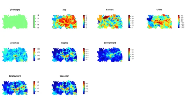
Figure 3: Plots of the interpolated covariates for the liver example.
so that,
R> class(popshape@data$pop)
[1] "ArealWeightedSum" "integer"
Next, we interpolate the covariate data onto the computational grid:
R> Zmat <- getZmat(formula = FORM, data = sd, regionalcovariates = popshape, + cellwidth = CELLWIDTH, ext = EXT, overl = polyolay)
As mentioned above, since we are using population as an explanatory variable, before we proceed to analyse the data we need to replace this covariate with the logarithm of population. This is because under a Poisson model, we expect the number of cases to be proportional to the population at risk (and not the exponential of population). Having interpolated the raw population counts above, we can now construct the logarithm as follows:
R> Zmat[, "pop"] <- log(Zmat[, "pop"])
R> Zmat[, "pop"][is.infinite(Zmat[, "pop"])] <- min( + Zmat[, "pop"][!is.infinite(Zmat[, "pop"])])
In the second line, we replace any zero population cell counts with the minimum value over the observation window; this avoids numerical problems handling negative infinite values. To see what the covariate data look like, we use
R> plot(Zmat)
According to Algorithm1, the next step is to define the population offset and priors. Since we are not using an offset in this example, we move onto defining the priors; note that more information on Poisson offsets together with an example are given in AppendixB.
The current version oflgcp allows two types of prior densities: a multivariate Gaussian prior forβ and a multivariate Gaussian prior on the log-scale for the positive parameters σ and φ
(and alsoθ in the spatiotemporal version) i.e.,
β ∼N(µβ,Σβ) and η={logσ,logφ} ∼N(µη,Ση).
We define these priors inlgcp as follows:
R> priors <- lgcpPrior(etaprior = PriorSpec(
+ LogGaussianPrior(mean = log(c(1, 500)), variance = diag(0.15, 2))), + betaprior = PriorSpec(
+ GaussianPrior(mean = rep(0, 9), variance = diag(10^6, 9))))
Note that the priors forη are always given in the order {logσ,logφ}. Lastly, we specify the initial values and choice of covariance function forY:
R> INITS <- lgcpInits(etainit = log(c(sqrt(1.5), 275)), betainit = NULL) R> cf <- CovFunction(exponentialCovFct)
It is not necessary to specify an initial value forη orβ as in the first line of code: by default, lgcp will initialise the MCMC using the prior mean for η, and for β it will initialise using the estimate obtained from an overdispersed Poisson glm fit of the cell counts against the covariates, and offset if appropriate. In the second line of code, we specify that the spatial dependence properties ofY should follow an exponential covariance function. For details on how to specify other sorts of covariance function, see AppendixC.
We are now in a position to run the MCMC algorithm. The following code runs the MALA chain for 1,000,000 iterations, with an initial burn-in of 100,000 iterations, followed by a further 900,000 iterations, of which every 900th sample is saved to disk. Note that the call to this function is not dissimilar to previous versions of the code, and we refer the reader to
Tayloret al. (2013), for an explanation of the options not discussed below.
R> BASEDR <- getwd()
R> lg <- lgcpPredictSpatialPlusPars(formula = FORM, sd = sd, Zmat = Zmat, + model.priors = priors, model.inits = INITS, spatial.covmodel = cf, + cellwidth = CELLWIDTH, poisson.offset = NULL, mcmc.control = mcmcpars( + mala.length = 1000000, burnin = 100000, retain = 900,
+ adaptivescheme = andrieuthomsh(inith = 1, alpha = 0.5, C = 1, + targetacceptance = 0.574)),
+ output.control = setoutput(gridfunction = dump2dir(
+ dirname = paste(BASEDR, "/liver/", sep = ""), forceSave = TRUE)), + ext = EXT)
R> save(list = ls(), file = file.path(BASEDR, "liver", "liver.RData"))
The last step in Algorithm 1is to perform diagnostic checks and then summarise the results: the package lgcpprovides functions to aid in this process.
0 200 400 600 800 1000 −20000 −15000 −10000 Iteration/900 log target
Figure 4: Diagnosing convergence to a posterior mode: a plot of the log target. Diagnostic checks include (1) checking that the Markov chain is mixing well and (2) checking convergence of the Markov chain. Establishing convergence for models of this class is difficult due to the fact that the target is high-dimensional: there are 32,779 parameters to estimate in this case. A simple, but effective method to check that the chain has converged to a posterior mode is to examine a plot of the log-target, log{π(β, η, Y|X)}+cup to an additive constantc:
R> plot(ltar(lg), type = "s", xlab = "Iteration/900", ylab = "log target")
the results of which appear in Figure4.
The plot shows that initially the chain was far away from a mode with the log-target having a value of around −6,000, but it quickly appears to have settled around values at about
−22,000; note that these values have been thinned by the same amount as the original chain. If this plot does not appear to have converged, then this indicates that the Markov chain has not converged, and needs to be run for a longer period of time.
We next check the mixing of the latent fieldY:
R> lagch <- c(1, 5, 15)
R> Sacf <- autocorr(lg, lagch, inWindow = NULL) R> for(i in 1:3) {
+ image.plot(xvals(lg), yvals(lg), Sacf[, , i], zlim = c(-1, 1), + axes = FALSE, xlab = "", ylab = "", asp = 1,
+ sub = paste("Lag:", lagch[i])) + plot(sd$window, add = TRUE) + scalebar(5000, label = "5 km") + }
which produces the plots in Figure 5. These plots show from left-to-right the lag 1, 5 and 15 cellwise autocorrelation in the Y chain. Note that producing such plots is only pos-sible if the chain has been dumped to disk (set using the dump2dir option in the call to lgcpPredictSpatialPlusPars).
Lag: 1 −1.0 −0.5 0.0 0.5 1.0 5 km Lag: 5 −1.0 −0.5 0.0 0.5 1.0 5 km Lag: 15 −1.0 −0.5 0.0 0.5 1.0 5 km
Figure 5: Left to right: lag 1, 5, 15 autocorrelation in the fieldY(j).
0 5 1015202530 0.0 0.2 0.4 0.6 0.8 1.0 Lag log ( σ ) 0 5 1015202530 0.0 0.2 0.4 0.6 0.8 1.0 Lag log ( φ ) 0 5 101520 2530 0.0 0.2 0.4 0.6 0.8 1.0 Lag β(Inte rc e p t ) 0 5 1015202530 0.0 0.2 0.4 0.6 0.8 1.0 Lag βpop 0 5 1015202530 0.0 0.2 0.4 0.6 0.8 1.0 Lag βprop m a le 0 5 101520 2530 0.0 0.2 0.4 0.6 0.8 1.0 Lag βInc o m e 0 5 1015202530 0.0 0.2 0.4 0.6 0.8 1.0 Lag βEm p lo y m e n t 0 5 1015202530 0.0 0.2 0.4 0.6 0.8 1.0 Lag βEd u c a ti o n 0 5 1015202530 0.0 0.2 0.4 0.6 0.8 1.0 Lag βBa rr ie rs 0 5 1015202530 0.0 0.2 0.4 0.6 0.8 1.0 Lag βCrim e 0 5 1015202530 0.0 0.2 0.4 0.6 0.8 1.0 Lag βEnv ir o n m e n t
Figure 6: Autocorrelation plots of the parameters β and η from the spatial point process model for PBC.
These plots show that there is very little autocorrelation in the sampledY(j). Similarly, we can produce autocorrelation plots for the parametersβ andηusingparautocorr(lg), shown in Figure 6; and trace plots using the command traceplots(lg), shown in Figure 7. For manual extraction of theβ and η chains, use betavals(lg)and etavals(lg)respectively. Having established satisfactory convergence of the chain, we can now proceed to making inferences from the model. We first produce a table of parameter estimates:
R> parsum <- parsummary(lg)
which can then be printed to the console by typingparsum. Alternatively, using
R> parsum <- parsummary(lg, LaTeX = TRUE) R> library("miscFuncs")
R> latextable(parsum, rownames = rownames(parsum),
+ colnames = c("Parameter", colnames(parsum)), digits = 4)
converts the output to a LATEX table, which can be copied and pasted into a LATEX document
0 200 400 600 800 0.5 0.6 0.7 0.8 0.9 Sample No. σ 0 200 400 600 800 500 1000 1500 Sample No. φ 0 200 400 600 800 −20 −18 −16 −14 −12 Sample No. β(Inte rc e p t ) 0 200 400 600 800 0.8 0.9 1.0 1.1 1.2 1.3 1.4 1.5 Sample No. βpop 0 200 400 600 800 −25 −20 −15 −10 −5 0 Sample No. βprop m a le 0 200 400 600 800 −6 −4 −2 0 2 4 Sample No. βInc o m e 0 200 400 600 800 −5 0 5 Sample No. βEm p lo y m e n t 0 200 400 600 800 −0.03 −0.02 −0.01 0.00 Sample No. βEduc a ti o n 0 200 400 600 800 −0.04 −0.02 0.00 Sample No. βBarrie rs 0 200 400 600 800 −0.6 −0.4 −0.2 0.0 0.2 0.4 Sample No. βCri m e 0 200 400 600 800 −0.02 0.00 0.01 0.02 0.03 0.04 Sample No. βEn v ir o n m e n t
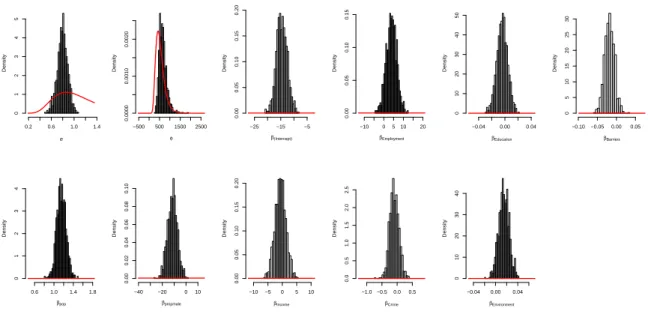
Figure 7: Trace plots of the parameters β and η from the spatial point process model for PBC. σ Density 0.2 0.6 1.0 1.4 0 1 2 3 4 5 φ Density −500 500 1500 2500 0.0000 0.0010 0.0020 β(Intercept) Density −25 −15 −5 0.00 0.05 0.10 0.15 0.20 βpop Density 0.6 1.0 1.4 1.8 0 1 2 3 4 βpropmale Density −40 −20 0 10 0.00 0.02 0.04 0.06 0.08 0.10 βIncome Density −10 −5 0 5 10 0.00 0.05 0.10 0.15 0.20 βEmployment Density −10 0 510 20 0.00 0.05 0.10 0.15 βEducation Density −0.04 0.00 0.04 0 10 20 30 40 50 βBarriers Density −0.10 −0.05 0.00 0.05 0 5 10 15 20 25 30 βCrime Density −1.0 −0.50.0 0.5 0.0 0.5 1.0 1.5 2.0 2.5 βEnvironment Density −0.04 0.00 0.04 0 10 20 30 40
Figure 8: Plots of the prior and posterior values of each parameter.
A LATEX formatted verbal summary of the table can also be produced:
R> textsummary(lg, digits = 4)
The output can be copied and pasted into a LATEX document and later edited by the user,
the result is shown in quote style below. In the user’s report, it remains to edit the text as desired and add details of the variables and units, where appropriate.
Parameter Median Lower 95% CRI Upper 95% CRI σ 0.7999 0.6033 0.9695 φ 637.1 389.3 1098 exp(β(Intercept)) 4.111×10⁻⁷ 8.735×10⁻⁹ 3.019×10⁻⁵ exp(βpop) 3.162 2.633 3.84 exp(βpropmale) 1.328×10⁻⁵ 3.937×10⁻⁹ 4.62×10⁻² exp(βIncome) 0.5449 1.425×10⁻² 23.05 exp(βEmployment) 52.73 0.2343 9981 exp(βEducation) 0.9961 0.9797 1.012 exp(βBarriers) 0.982 0.9594 1.007 exp(βCrime) 0.9034 0.6956 1.223 exp(βEnvironment) 1.015 0.9967 1.035
Table 1: Parameter estimates for the LGCP point pattern model for the PBC data. A summary of the parameters of the latent field is as follows. The parameter σ
had median 8×10⁻¹ (95% CRI 0.603 to 0.97) and the parameter φ had median 637 (95% CRI 389 to 1098).
The following effects were found to be significant: each unit increase inpropmale led to a reduction in relative risk with median 1.33×10⁻⁵ (95% CRI 3.94×10⁻⁹ to 4.62×10⁻²); each unit increase in pop led to a increase in relative risk with median 3.16 (95% CRI 2.63 to 3.84).
The remainder of the main effects were not found to be significant: each unit increase inIncome led to a reduction in relative risk with median 0.545 (95% CRI 1.42×10⁻² to 23); each unit increase in Education led to a reduction in relative risk with median 0.996 (95% CRI 0.98 to 1.01); each unit increase inBarriersled to a reduction in relative risk with median 0.982 (95% CRI 0.959 to 1.01); each unit increase in Crimeled to a reduction in relative risk with median 0.903 (95% CRI 0.696 to 1.22); each unit increase in Employmentled to a increase in relative risk with median 52.7 (95% CRI 0.234 to 9981); each unit increase inEnvironment led to a increase in relative risk with median 1.01 (95% CRI 0.997 to 1.03).
It is also of interest to examine plots of the prior and posterior distributions of the parameters. This is particularly important to help us interpret of the posterior density of the spatial scale parameter, φ, which tends not to be well identified by the data, see Zhang (2004) for an example in the classical geostatistical context. Typing
R> priorpost(lg)
produces the plots in Figure 8. These plots confirm that whilst the covariate effects, β, are well identified by the data, the parameters of the process Y are not so well identified. The parameter σ shows a greater departure from the prior compared with the parameter φ; one must therefore exercise caution in making strongly probabilistic inferential statements about these parameters, since they appear to be influenced by the prior.
Next we produce a plot of the posterior covariance function using:
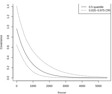
0 1000 2000 3000 4000 5000 0.0 0.2 0.4 0.6 0.8 1.0 Range Co v ar iance
Figure 9: Plot of the posterior estimated covariance function ofY.
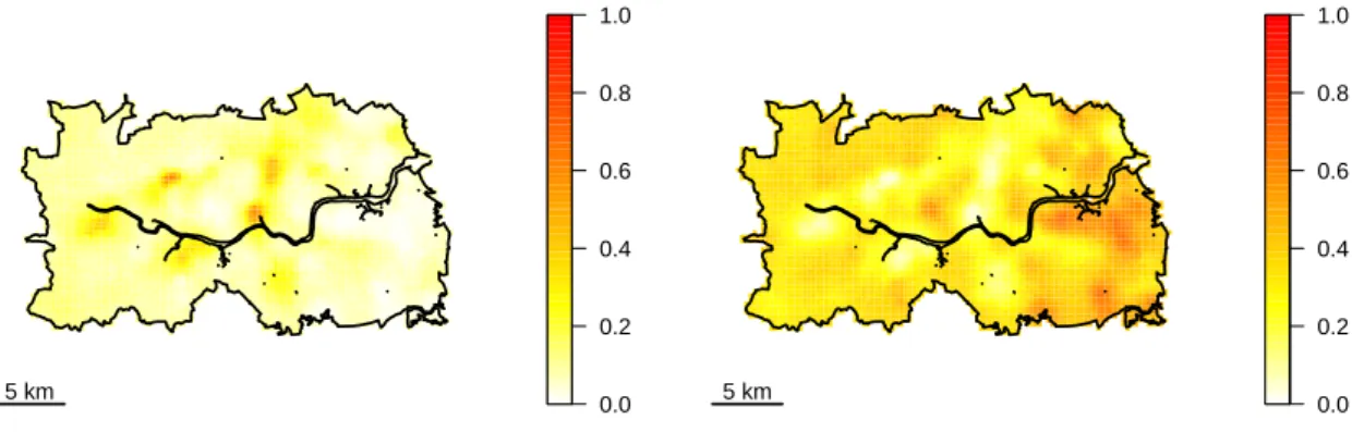
0.0 0.2 0.4 0.6 0.8 1.0 5 km 0.0 0.2 0.4 0.6 0.8 1.0 5 km
Figure 10: Left: Plot of the posterior probability that the relative risk exceeds 2. Right: Plot of the posterior probability that the relative risk is below 0.5. Note that by setting sub = NULL, or omitting subfrom the call toplotExceed above, the threshold will be printed as a subtitle in each of the plots (i.e., printing the threshold as a subtitle is the default behaviour forplotExceed).
the results are shown in Figure9.
Finally, it is also of interest in epidemiology to understand if there are some spatial areas of (covariate-adjusted) particularly high or low incidence. These exceedance (or respectively lower-tail exceedance) probabilities, are P{exp(Y) > k|X} or P{exp(Y) < k|X} for a pre-specified thresholdk. These quantities can be expressed as a posterior expectation,
P[exp(Y)> k|X] =Eπ(β,η,Y|X){I[exp(Y)> k]}=
1 n n X i=1 I[exp(Y(i))> k],
whereI is the indicator function. We use theexceedProbsfunction to set up these probabil-ities andlgcp:::expectation.lgcpPredictto compute the Monte Carlo expectation; note that an explicit call tolgcp:::expectation.lgcpPredict is necessary here as in the latest
version of lgcp there is a new method expectation for functions of β, η and Y for objects generated by the functionlgcpPredictSpatialPlusPars. See Appendix Dfor examples of more complex expectations. The code below generates the plots in Figure10.
R> ep <- exceedProbs(c(1.5, 2, 5, 10))
R> sp <- exceedProbs(c(2/3, 1/2, 1/5, 1/10), direction = "lower") R> ex <- lgcp:::expectation.lgcpPredict(lg, ep)
R> su <- lgcp:::expectation.lgcpPredict(lg, sp)
R> plotExceed(ex[[1]], "ep", lg, zlim = c(0,1), asp = 1, + axes = FALSE, xlab = "", ylab = "", sub = "")
R> scalebar(5000, label = "5 km")
R> plotExceed(su[[1]], "sp", lg, zlim = c(0, 1), asp = 1, + axes = FALSE, xlab = "", ylab = "", sub = "")
R> scalebar(5000, label = "5 km")
4.2. PBC in Newcastle-Upon-Tyne, an aggregated count model
Introduction to continuous models for areal count data
Now suppose that instead of observing the exact location of events we instead observeTi, the
total number of cases in regionAi, whereAi∩Aj =∅ fori=6 j,Smi=1Ai =W and W is the
observation window; see Figure11.
Aggregated exposure or outcome data are often used because individual-level information is not available for economic or confidentiality reasons (Beale, Abellan, Hodgson, and Jarup
2008; Diggle, Guan, Hart, Paize, and Stanton 2010). Area-level analyses are prone to
so-called ‘ecological bias’ (Wakefield and Lyons 2010; Wakefield, Haneuse, Dobra, and Teeple 2011); the name refers to differences in effect sizes that result from modelling association
Figure 11: Plot of cases of primary biliary cirrhosis in Newcastle-Upon-Tyne, case counts aggregated to regions.
simultaneous autoregressive models. Whilst aggregated count models such as these are com-putationally quick to fit, there is an argument against using them when the regions are quite varied in shape and size, as the definition of what it means to be a neighbour is then somewhat contrived and can lead to undesirable properties in parameter estimates, seeWall(2004). Other authors e.g.,Mølleret al.(1998),Brix and Diggle(2001) andDiggleet al.(2005a), take the intuitively more natural approach of modelling variation in risk as a spatially continuous process, but their methods do not directly handle areal data. Kelsall and Wakefield (2002) model area-level counts as a product of the expected number of counts (based on population demography) and a relative risk term, which they model as a spatially continuous log-Gaussian process, from which they were able to compute covariances between regions accounting for each region’s size and shape.
Our aim in the present article is to fit a model of the form given in Equation5to areal count data: the number of eventsTi in each region Ai. In this case, it is not only Y,η and β that
are unknown, but also the event counts in each computational grid cell. In order to proceed, we use the technique of data augmentation, seevan Dyk and Meng(2001) for a review. We augment the list of parameters,{β, η, Y}, with an additional variableN, the cell counts and sample from,
π(β, η, Y, N|T1, . . . , Tm).
This can be achieved using a Gibbs scheme, alternately sampling fromπ(β, η, Y|N, T1:m) and π(N|β, η, Y, T1:m), see Li, Brown, Gesink, and Rue (2012) and Diggle et al. (2013). Note
that the random variable N is akin to the observed data X in Equation 5. Conditional independence properties imply that
π(β, η, Y|N, T1:m) =π(β, η, Y|N).
We sample from this density using exactly the same MALA algorithm as for the spatial point process. The densityπ(N|β, η, Y, T1:m) turns out to be multinomial, and so is straightforward
to sample from. Of critical importance to the data augmentation is the way in which lgcp handles the polygon/polygon overlay operations: each non-trivial intersection between the computational grid cells and the SpatialPolygonsDataFrame is computed, allowing accu-rate sampling fromπ(N|, β, η, Y, T1:m). Although straightforward in principle, sampling from π(N|β, η, Y, T1:m) nevertheless incurs a computational cost. Rather than doing this every
it-eration, the MCMC function for aggregated data,lgcpPredictAggregateSpatialPlusPars, has an argumentNfreq, which allow the user to set this frequency; by default, this is set to draw a newN ∼π(N|β, η, Y, T1:m) every 101 iterations.
Areal count data in lgcp
We now discuss how to fit a spatially continuous log-Gaussian Cox process model to areal count data. These data were contained in aSpatialPolygonsDataFrameobject spdf,
R> load("liver_spdf.RData") R> spdf
class : SpatialPolygonsDataFrame nfeatures : 177
extent : 409144.1, 439753.8, 556265.4, 574219.4 (xmin, xmax, ymin, ymax) coord. ref. : NA nvariables : 1 names : X min values : 0 max values : 24
a plot of these data is in Figure 11. The object spdf has a columnX containing the event counts in each polygon.
We initially used the sameCELLWIDTHandEXTparameters as for the point process version of our model. However, in pilot runs it became apparent that for this model, we needed to use a larger value of EXT, see Appendix Efor details on this matter. Otherwise, we used the same formula, FORM; priors, priors; and covariance function,cf, as in the point process version of this model discussed in the previous section. This allows us to compare inferences where the point locations are known and where the point locations are unknown.
For this example, we did not use minimum contrast methods to obtain initial estimates of the parameters. Had the collection of polygons inspdfbeen on a sufficiently fine scale to capture spatial variation in population reasonably well, then the function spSamplecould have been used to impute cases into the observation window, from which minimum contrast estimates could have been obtained using minimum.contrast as before. However, in this instance the set of polygons do not capture this fine scale variation, so we instead opt to initialise the MCMC algorithm using the prior mean.
Running the following commands,
R> CELLWIDTH <- 300 R> EXT <- 3
R> polyolay <- getpolyol(data = spdf, cellwidth = CELLWIDTH, + regionalcovariates = popshape, ext = EXT)
R> Zmat <- getZmat(formula = FORM, data = spdf, cellwidth = CELLWIDTH, + regionalcovariates = popshape, ext = EXT, overl = polyolay)
R> Zmat[, "pop"] <- log(Zmat[, "pop"])
R> Zmat[, "pop"][is.infinite(Zmat[, "pop"])] <- min( + Zmat[, "pop"][!is.infinite(Zmat[, "pop"])])
sets up the polygon/polygon overlay and performs interpolation onto the computational grid and replaces population with log-population as in the point process model.
The function call to run the MCMC routine is:
R> BASEDR <- getwd()
R> lg <- lgcpPredictAggregateSpatialPlusPars(formula = FORM, spdf = spdf, + Zmat = Zmat, overlayInZmat = FALSE, model.priors = priors,
+ spatial.covmodel = cf, cellwidth = CELLWIDTH, mcmc.control = mcmcpars( + mala.length = 3100000, burnin = 100000, retain = 3000,
+ adaptivescheme = andrieuthomsh(inith = 1, alpha = 0.5, C = 1, + targetacceptance = 0.574)),