GAN-based Generation and Automatic Selection of Explanations for Neural Networks

GAN-

BASED

G

ENERATION AND

A

UTOMATIC

S

ELEC

-TION OF

E

XPLANATIONS FOR

N

EURAL

N

ETWORKS

Saumitra Mishra*, Daniel Stoller*, Emmanouil Benetos* #, Bob L. Sturm†& Simon Dixon* *_{School of EECS, Queen Mary University of London, UK}

#_{The Alan Turing Institute, UK}

†_{Speech, Music and Hearing, KTH Royal Institute of Technology, Sweden}

{saumitra.mishra, d.stoller, emmanouil.benetos_}@qmul.ac.uk,

[email protected], [email protected]

A

One way to interpret trained deep neural networks (DNNs) is by inspecting char-acteristics that neurons in the model respond to, such as by iteratively optimising the model input (e.g., an image) to maximally activate specific neurons. However, this requires a careful selection of hyper-parameters to generate interpretable ex-amples for each neuron of interest, and current methods rely on a manual, quali-tative evaluation of each setting, which is prohibitively slow. We introduce a new metric that uses Fr´echet Inception Distance (FID) to encourage similarity between model activations for real and generated data. This provides an efficient way to evaluate a set of generated examples for each setting of hyper-parameters. We also propose a novel GAN-based method for generating explanations that enables an efficient search through the input space and imposes a strong prior favouring re-alistic outputs. We apply our approach to a classification model trained to predict whether a music audio recording contains singing voice. Our results suggest that this proposed metric successfully selects hyper-parameters leading to interpretable examples, avoiding the need for manual evaluation. Moreover, we see that ex-amples synthesised to maximise or minimise the predicted probability of singing voice presence exhibit vocal or non-vocal characteristics, respectively, suggest-ing that our approach is able to generate suitable explanations for understandsuggest-ing concepts learned by a neural network.

1

I

There is an increasing interest in interpreting black-box machine learning models, especially Deep Neural Networks (DNNs) (Doshi-Velez & Kim, 2017). Insights about how models function can assist in gaining trust in their predictions – an essential factor for model adoption in safety-critical applications (e.g. health care, self-driving cars) (Ribeiro et al., 2016b). We can understand a ma-chine learning model by employing one of two strategies. The first involves training inherently interpretable models and is a promising research direction, but often such models perform poorly when compared to state-of-the-art black-box models (Ribeiro et al., 2016a). In contrast, the second strategy involves a post-hoc analysis of a trained model, which does not require compromises on its predictive capacity.

There are two key approaches to bring post-hoc interpretability to DNNs in particular (Montavon et al., 2018). The first focuses on explaining the predictions of a model (Simonyan et al., 2014; Bach et al., 2015; Ribeiro et al., 2016b) for a given input, while the second analyses components (e.g. neurons or layers) of a DNN (Olah et al., 2017). We focus on the second approach in this paper, as it yields general insights about how a DNN forms its predictions.

We can analyse components of a DNN using different methodologies. For example, one can use feature inversion to map latent codes to the input space highlighting the discriminative information a DNN preserves at its layers (Mahendran & Vedaldi, 2015; Dosovitskiy & Brox, 2016). In another direction, one can analyse features that different components of a DNN are sensitive to. One way

z x fa

Noise Generator Example Classifier Calculate

a ∇z a Response ∇zpz pz Gradient +

(pre-trained) (pre-trained) response

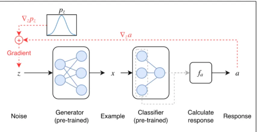
Figure 1: Overview of our proposed approach. A noise vectorzis used to generate an examplex, for which a responsea_∈Ris calculated with a response functionfafrom all neuron activations of

the classifier. facan be defined depending on which aspect of the classifier is of interest; examples

include the activation of a certain neuron, or the average layer activation.zis optimised to maximise the responsea, but also the prior probabilitypz(z)to favour realistic outputs.

to do this is by identifying instances from the dataset that maximally activate different components in a DNN (Zhou et al., 2015). Another way is by using Activation Maximisation (AM) (Erhan et al., 2009) that iteratively optimises random noise to synthesise examples in the input space (e.g., images) to maximally activate a neuron or layer in a DNN. Since AM is data-independent and tends to focus more on the explanatory input factors, we will pursue an AM-based approach in this paper. The interpretability of examples generated by AM depends on two key factors: optimisation of hyper-parameters and the prior. Generally, interpretable examples are selected for each neuron by performing a grid search in the hyper-parameter space and visually inspecting each generated exam-ple (Nguyen et al., 2016a), but this is subjective, prohibitively slow and limits the hyper-parameter search space. Also, such an approach is not scalable to analysing other DNN neurons that may require different hyper-parameter settings.

The use of priors for AM restricts the input search space to prevent generating uninformative, ad-versarial examples. Researchers have proposed several hand-crafted priors for effective AM, syn-thesising interpretable images (Yosinski et al., 2015; Nguyen et al., 2016b; Mahendran & Vedaldi, 2015). In another direction, Nguyen et al. (2016a) demonstrated that replacing hand-crafted priors by a learned prior (adversarially trained feature inverter) considerably improves the interpretability of synthesised images. However, their approach requires training a separate prior for each layer in the classifier, and appears to rely on the prior and the classifier model having similar architectures. In this work, we aim to tackle these challenges, making the following contributions:

• To our knowledge, we are the first to use a Generative Adversarial Network (GAN) for example generation using AM. This imposes a strong prior and enables effective AM for any given part of a classifier and even other classifiers with the same input domain without re-training the generator. The work by Nguyen et al. (2017) is closest to ours, in which the authors use a denoising autoencoder as a prior on the latent code of the adversarially trained feature inverter.

• We propose a quantitative measure estimating the interpretability of a set of generated examples by adopting the Fr´echet Inception Distance (FID) metric (Heusel et al., 2017). We provide evidence for its effectiveness by qualitatively analysing the synthesised examples.

• We apply our method to a state-of-the-art deep audio classification model that predicts singing voice activity in music excerpts. This results in visualisations that successfully capture the concept represented by the ground truth labels the classifier was trained to predict. There have been some recent works in understanding deep audio classification models, but they either use a different method (Mishra et al., 2018) or perform AM with hand-crafted priors (Zhang & Duan, 2018; Krug & Stober, 2018).

2

M

Figure 1 provides an overview of our method. For a pre-trained neural network classifierfcwithM

neurons and inputx_∈ Rd, our goal is to provide examples that activate a given neuron activation

pattern (“classifier response”). Formally, we definefn(x)∈RM as the output activations ofallM

neurons in the classifierfcfor a given input examplex. The classifier response we aim to explain can

then be defined in a general fashion as the output of some functionfa :RM →Rthat takesallM

neuron activations of the classifier as input.facan be set to output the activation of a single neuron,

or the average activation of one or multiple layers, but any differentiable function is supported.

2.1 ACTIVATION MAXIMISATION

We can perform activation maximisation to find an input example xˆ _{∈ R}d _{so that the resulting}

activationfa(_·)is maximised:

ˆ

x= arg max

x

fa(fn(x)) (1)

The above objective can be optimised by stochastic gradient descent (SGD) by backpropagating through the classifier layers.

2.2 GAN-BASED PRIOR

However, activation maximisation often produces adversarial examples (Nguyen et al., 2015), which can be very different from inputs encountered during classifier training and testing, are hard to interpret and do not explain the classifier’s behaviour for real-world inputs. Furthermore, optimising over the inputxdirectly is often difficult, especially if the dimensionalitydis high (Nguyen et al., 2016a).

Our method makes use of a GAN (for more details, see Goodfellow et al. (2014)), where a generator fg:Rn→Rdis trained to map a noise vectorz∈Rndrawn from a known noise distributionpzto

a generated examplex, and optimises

ˆ

z= arg max

z

fa(fn(fg(z))) +λlogpz(z). (2)

The weighting termλ _≥0is a hyper-parameter controlling the trade-off between activation max-imisation and the realism of the generated examples. Note that we search in the low-dimensional noise space for a vectorˆzwhose associated generator outputfg(ˆz)produces a high activation, which avoids optimisation issues. To encourage realistic outputs, the real data densitypx should ideally

be used in the form of a prior termlogpx(fg(z))in equation 2, but we do not have access topx.

However, assuming a well-trained generator, we can uselogpz(z)instead, since it should be

ap-proximately proportional.

To optimise equation 2 with gradient descent, we requirepz to be a continuously differentiable

distribution. Note that this does not include the uniform distribution commonly used for training GANs, for example in (Goodfellow et al., 2014; Radford et al., 2015; Hjelm et al., 2017).

2.3 EXAMPLE GENERATION

The previous section 2.2 demonstrated how one example is generated in our approach. To generate a set ofNexamples, we drawNrandom noise vectorsz˜1, . . . ,z˜N independently frompzas

initial-isation points for SGD. The resulting examples should be diverse, so converging to the same optima of equation 2 independent of initialisation is undesirable. Therefore we set the SGD learning ratelr

as well as the number of update stepsNtas hyper-parameters, since they control the influence of the

initialisation points on the generated examples and thereby the amount of diversity and randomness.

2.4 HYPER-PARAMETER OPTIMISATION

To optimise the prior weightλand optimisation parameterslras well asNt, it would be ideal to

have human subjects evaluate the usefulness of the explanations resulting from different configura-tions, but this is prohibitively time-intensive. Therefore, we introduce a novel, automatic metric for quickly evaluating a set of generated explanations, allowing efficient hyper-parameter optimisation.

Classifier responsefa(·) Probability px ˆ px pg1 pg2 pg3 pg4

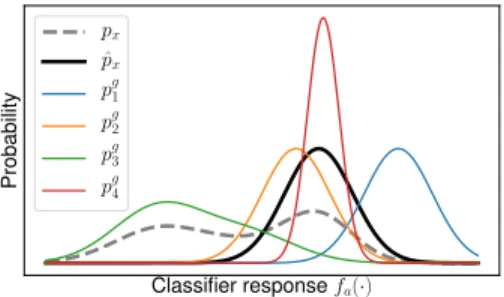
Figure 2: Intuitive explanation for our proposed metric, showing the distributions of activations fa(·)obtained for input examples from the dataset (px), of the dataset examples with the highestN

responsesfa(_·)(pˆx), and of four hypothetical generators,pg1, . . . .p

g

4. Our metric determines which

generator distribution is most similar topˆxto ensure realistic examples.

In the following, we will explain our reasoning using the hypothetical example in Figure 2. We posit that good interpretability requires the generated examples to have a similar distribution of classifier responsesfa(·)as theN samples with the highest response from the dataset (pˆxin Figure 2). This

is because unrealistic adversarial examples (generator1in Figure 2) often lead to large responses. Also, too much weight on the GAN priorλor ineffective optimisation (generator3) leads to ex-amples that are realistic, but have too low responses compared to real exex-amples. Additionally, the variance of responses should be similar (making generator2 the best according to our metric) to ensure a sufficient degree of diversity in the generated samples (in contrast to generator4).

To take the average and the variance of the responses into account, we therefore adopt the Fr´echet Inception Distance (FID) (Heusel et al., 2017) as our distance metric. Since our responsesfa for

each example are scalar values, the FID reduces to

D((µr, σr),(µg, σg)) = (µr−µg)2+σr+σg−2(σrσg)

1

2, (3)

whereµrandµgare the means andσrandσgthe unbiased sample variance of the (one-dimensional)

real and the generated response distribution, respectively.

In the following section 3, we will investigate whether the metric proposed above adequately reflects how useful the set of generated examples is to a human observer.

3

E

To evaluate our method and to investigate whether approaches based on AM can transfer to domains other than computer vision, we apply it to audio classification. Specifically, we will consider Singing Voice Detection (SVD), a binary classification task (Lee et al., 2018) where a classifier predicts whether singing voice (vocals) is present in a segment of a music recording.

3.1 CHOICE OF CLASSIFIER

We select a state-of-the-art SVD model1 introduced by Schl¨uter & Grill (2015). The model is an eight-layer Convolutional Neural Network (CNN) the architecture of which is mentioned in Ap-pendix (Table 4). It takes a Mel spectrogram of an audio excerpt of1.6s duration as input. The Mel spectrogram is calculated by first applying an FFT2_{and taking the magnitudes of the resulting} spec-trum. Later, we apply a Mel filterbank3_{to summarise the energies across different frequency bands.} Finally, we normalise the resulting non-negative values by applyingx_→log(max(x,10−7)). Using a single neuron with sigmoid activation in the last layer, the CNN predicts the probability of singing voice being present at the centre of the input audio excerpt. Schl¨uter & Grill (2015) train the model

1

Available as open source athttps://github.com/f0k/ismir2015

2_{Using a window size of1024and a hop size of315samples, with audio sampled at22050Hz} 3

The Mel filterbank is a set of band-pass filters distributed along the Mel-frequency scale, which is a per-ceptual scale of pitch defining a logarithmic relationship between frequency and perceived pitch. We use80 filters in our work, ranging from27.5to8000Hz.

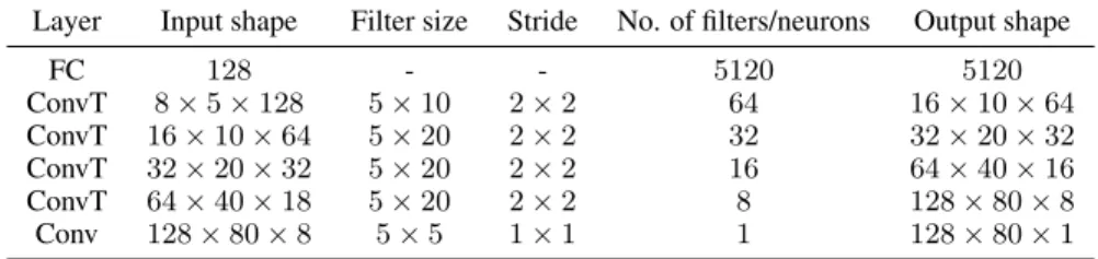
Table 1: The architecture of our generator. The transposed convolutional layers (ConvT) as well as the FC layer have LeakyReLU activations.

Layer Input shape Filter size Stride No. of filters/neurons Output shape

FC 128 - - 5120 5120 ConvT 8×5×128 5×10 2×2 64 16×10×64 ConvT 16×10×64 5×20 2×2 32 32×20×32 ConvT 32×20×32 5×20 2×2 16 64×40×16 ConvT 64×40×18 5×20 2×2 8 128×80×8 Conv 128×80×8 5×5 1×1 1 128×80×1

in a supervised fashion by minimising the binary cross-entropy loss between model predictions and the ground-truth labels.

As training input, the authors randomly sample excerpts from the 93 French Pop music songs con-tained in the Jamendo dataset (Ramona et al., 2008). The dataset is pre-partitioned into subsets of 61 (training), 16 (validation) and 16 (testing) songs, respectively, and each song has manual annotations indicating the start and end times of each vocal segment.

We replicated the proposed approach of the authors4_{, obtaining a classifier whose performance is} very similar to the one reported by the authors, as shown in Appendix (Table 3).

3.2 CHOICE OF RESPONSE FUNCTION

In this study, we focus on generating positive and negative examples that maximally or minimally excite the final output neuron of the classifier, respectively. Compared to using other definitions of fa, this allows us to directly evaluate the characteristics of our generated examples, as the positive

examples should differ from the negative ones by the presence of singing voice since the classifier is known to be accurate at singing voice detection.

Our initial experiments show that the predicted probability converges to0or1after only very few it-erations, leading to vanishing gradients due to saturation of the sigmoid non-linearity, effectively halting optimisation. We argue this indicates an inherent problem of the classifier and not our method, as neural networks are well-known to be prone to making over-confident predictions (Gal & Ghahramani, 2016). Thus, we applied our method to the pre-sigmoid activations of the final neuron instead.

3.3 GANTRAINING

We use the FMA dataset (Defferrard et al., 2017) for training the GAN, selecting only Pop music pieces to reduce the data complexity and to make the song selection more similar to the one used for training the classifier. The audio signals are converted to Mel spectrograms, replicating the classifier preprocessing described in section 3.1. From each song’s full spectrogram, we create clips with115

time frames and an equal amount of spacing between each clip.

For the generator, we choose a standard normal likelihood_N(z_|0n;In)for the continuously

differ-entiable noise termpz(z), with a dimensionality ofn= 128. The generator architecture is a CNN adapted from the DCGAN (Radford et al., 2015) and is shown in Table 1, using multiple strided transposed convolutions. The final convolution outputs a128_×80_×1tensor, which is cropped evenly at the borders to obtain115time frames as required by the classifier. The final convolution employsx_→max(x,log(10−7))as activation function to ensure the generated spectrogram magni-tudes are in the same interval range as the Mel spectrograms obtained from preprocessing real audio samples following section 3.1.

4

The open-sourced version of the classifier introduced by Schl¨uter & Grill (2015) is based on Theano and Lasagne and was ported to Tensorflow as part of this work

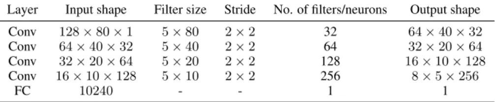
Table 2: The architecture of our discriminator. Convolutional layers have LeakyReLU activations and bias. The fully connected layer has no bias or activation function.

Layer Input shape Filter size Stride No. of filters/neurons Output shape

Conv 128×80×1 5×80 2×2 32 64×40×32

Conv 64×40×32 5×40 2×2 64 32×20×64

Conv 32×20×64 5×20 2×2 128 16×10×128

Conv 16×10×128 5×10 2×2 256 8×5×256

FC 10240 - - 1 1

The discriminator is again similar to the DCGAN (Radford et al., 2015) and is shown in Table 2, making use of multiple strided 2D convolutions to process the Mel spectrogram input of size115_× 80_×1. The output is a scalar real value used to distinguish real from generated samples.

We use the WGAN-GP objective for training our GAN as in (Gulrajani et al., 2017), with a GP weight of10. The Adam optimiser with a learning rate of10−4 _{is used to train the generator and}

discriminator for 600,000 iterations with a batch size of16.

3.4 AM OPTIMISATION

We perform a grid search over our hyper-parameters, using lr ∈ {0.1,0.01,0.001}, λ ∈ {0.1,0.01,0.001_} andNt ∈ {100,500,1000}, giving 27possible settings. We sampleN = 50

noise vectors from the noise distributionpz, resulting inN = 50examples along with their

respec-tive activation valuesfa(·)for each setting after applying our method. Also we feed the training

dataset to the classifier and record the last neuron activation for each excerpt, and select the top N = 50excerpts with maximum activation. We generate a new excerpt of 115consecutive Mel spectrogram frames (=1_b .6sec) for every50time frames (=0_b .7sec) in a recording. We optimise our objective in equation 2 by using the Adam optimiser withβ1= 0.99,β2= 0.999and= 10−8.

4

R

In section 4.1, we analyse the effectiveness of our metric proposed in section 2.4 in the context of hyper-parameter optimisation, before employing the best configuration to evaluate our explanation generation system in section 4.2.

4.1 HYPER-PARAMETER OPTIMISATION

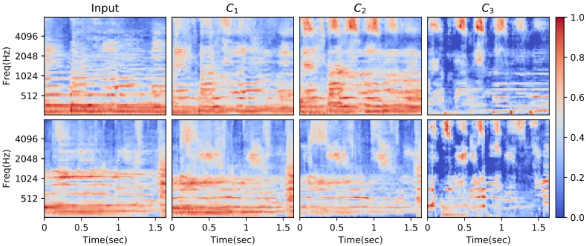
We investigate whether our evaluation metric reflects the quality of the results obtained for different hyper-parameter settings. Figure 3 shows the GAN output for two randomly sampled initial noise vectorsz˜1,z˜2and the corresponding results after maximising the last neuron activation using three

different hyper-parameter configurationsC1,C2andC3. In our best configurationC1, only small

changes are made to the initial output, which ensures diverse and realistic outputs due to the random values of˜zand high likelihood under the priorpz, while still increasing the response effectively. The

median configurationC2leads to further increased harmonic as well as high-frequency energy,

al-though to a slightly unrealistic extent, and configurationC3produces extremely sparse outputs with

maximum energies one magnitude greater than those found in real spectrograms, and unrealistically high responses of up to78, thus is ineffective. This shows our metric can rank the different hyper-parameter settings with respect to how useful the resulting explanations are for a human observer. Further perceptual studies are left for future work to establish a stronger connection.

4.2 QUALITATIVE ANALYSIS OF EXPLANATIONS

We use the configurationC1(Table 5 in Appendix) to produce positive and negative examples for the

last output neuron of our vocal classifier by maximising or minimising its activation, respectively. Since the classifier was trained to distinguish vocal from non-vocal audio, this allows us to

investi-512 1024 2048 4096 Freq(Hz) Input C1 C2 C3 0 0.5 1 1.5 Time(sec) 512 1024 2048 4096 Freq(Hz) 0 0.5 1 1.5 Time(sec) 0 0.5 1 1.5 Time(sec) 0 0.5 1 1.5 Time(sec) 0.0 0.2 0.4 0.6 0.8 1.0

Figure 3: Mel spectrogram visualisations demonstrating the effectiveness of our example evaluation metric from section 2.4, each normalised in scale independently so that red colors show relatively high and blue colors show relatively low spectral energy. The leftmost column shows the output of our GANfg(˜zi)for two initial noise vectorsz˜1,z˜2(one per row). The others show the result of

applying our method with hyper-parameter configurationsC1, C2andC3, which represent the best,

median and worst configuration from the set of27configurations according to our evaluation metric, respectively. For more details about the configurations, refer to Table 5 in the Appendix.

512 1024 2048 4096 Input Freq(Hz) 512 1024 2048 4096 Maximisation Freq(Hz) 0 0.5 1 1.5 Time(sec) 512 1024 2048 4096 Minimisation Freq(Hz) 0 0.5 1 1.5 Time(sec) 0 0.5 1 1.5 Time(sec) 0 0.5 1 1.5 Time(sec) 0.0 0.2 0.4 0.6 0.8 1.0

Figure 4: Mel spectrogram visualisations illustrating the concepts the neuron in the output layer of the classifier learns, each normalised in scale independently so that red colors show relatively high and blue colors show relatively low spectral energy. The top row represents initial GAN outputs fg(˜zi)for four initial noise vectorsz˜1,z˜2,˜z3,z˜4. The second and third rows represent examples

synthesised by maximally and minimally activating the output neuron. Table 6 in the Appendix details the activations from the last layer neuron for each visualisation depicted above.

gate whether our method can successfully capture the concept of vocal presence using its positive examples, and the concept of pure accompaniment using its negative examples.

Figure 4 shows four pairs of positive and negative examples, each generated using the same noise vectorz˜as initialisation point. We observe a stronger presence of harmonic content in the posi-tive examples, a lack of energy in the very low frequency band below the human voice range, and few transient sounds such as drum hits (visible as vertical bars), indicating our positive explana-tions indeed have many characteristics typical to vocal content. In contrast, the negative examples

have stronger transients and more bass frequency content, indicating the successful generation of purely instrumental examples. Since initial listening tests of the resynthesised audio confirms these observations, this suggests that our GAN-based approach can provide explanations useful for un-derstanding the concepts acquired by a neural network. Furthermore, Table 6 demonstrates that our method effectively optimises the response in all cases. A more quantitative, large-scale listening test is left for future work.

5

C

In this paper, we presented a GAN-based approach for efficiently generating inputs to a classifier so that its response is maximised, while maintaining realism thanks to its strong prior. Compared to previous approaches, it can be applied more flexibly to new classifiers and to excite different neurons in a classifier. We validated our method on a pre-trained singing voice classifier, showing it can retrieve the concept of singing voice presence encoded in the last output neuron. We presented a metric for automatic evaluation of the usefulness of a set of generated explanations, and use it for optimising the hyper-parameters of our approach. We qualitatively showed that our metric favours the subjectively more interpretable settings. For future work, we plan to conduct listening tests that present generated examples and require the prediction of the model’s behaviour for unseen inputs to quantify the interpretability of the explanations.

ACKNOWLEDGMENTS

DS is funded by EPSRC grant EP/L01632X/1. EB is supported by RAEng Research Fellowship RF/128 and a Turing Fellowship. This work is supported by EPSRC grant EP/R01891X/1.

R

Sebastian Bach, Alexander Binder, Gr´egoire Montavon, Frederick Klauschen, Klaus-Robert M¨uller, and Wojciech Samek. On Pixel-Wise Explanations for Non-Linear Classifier Decisions by Layer-Wise Relevance Propagation.PloS ONE, 10(7), 2015.

Micha¨el Defferrard, Kirell Benzi, Pierre Vandergheynst, and Xavier Bresson. FMA: A Dataset for Music Analysis. InProceedings of the 18th International Society for Music Information Retrieval Conference, (ISMIR), pp. 316–323, 2017.

Finale Doshi-Velez and Been Kim. Towards a Rigorous Science of Interpretable Machine Learning.

arXiv e-prints, arXiv:1702.08608, 2017.

Alexey Dosovitskiy and Thomas Brox. Inverting Visual Representations with Convolutional Net-works. InProceedings of the IEEE Conference on Computer Vision and Pattern Recognition, (CVPR), 2016.

Dumitru Erhan, Yoshua Bengio, Aaron Courville, and Pascal Vincent. Visualising Higher-Layer Features of a Deep Network. Technical Report 1341, University of Montreal, June 2009. Yarin Gal and Zoubin Ghahramani. Dropout as a Bayesian Approximation: Representing Model

Uncertainty in Deep Learning. InProceedings of the 33rd International Conference on Machine Learning, (ICML), pp. 1050–1059, 2016.

Ian Goodfellow, Jean Pouget-Abadie, Mehdi Mirza, Bing Xu, David Warde-Farley, Sherjil Ozair, Aaron Courville, and Yoshua Bengio. Generative Adversarial Nets. InProceedings of the 28th Annual Conference on Neural Information Processing Systems (NeurIPS), pp. 2672–2680, 2014. Ishaan Gulrajani, Faruk Ahmed, Mart´ın Arjovsky, Vincent Dumoulin, and Aaron C. Courville.

Im-proved Training of Wasserstein GANs. arXiv e-prints, arXiv:1704.00028, 2017.

Martin Heusel, Hubert Ramsauer, Thomas Unterthiner, Bernhard Nessler, and Sepp Hochreiter. Gans trained by a two time-scale update rule converge to a local nash equilibrium. InProceedings of the 30th Annual Conference on Neural Information Processing Systems (NeurIPS), pp. 6629– 6640, 2017.

R. Devon Hjelm, Athul Paul Jacob, Tong Che, Kyunghyun Cho, and Yoshua Bengio. Boundary-Seeking Generative Adversarial Networks. arXiv e-prints, 1702.08431, 2017.

Andreas Krug and Sebastian Stober. Introspection for Convolutional Automatic Speech Recogni-tion. In Proceedings of the Workshop: Analyzing and Interpreting Neural Networks for NLP, BlackboxNLP@EMNLP, pp. 187–199, 2018.

Kyungyun Lee, Keunwoo Choi, and Juhan Nam. Revisiting Singing Voice Detection: A Quantitative Review and the Future Outlook. In Proceedings of the 19th International Society for Music Information Retrieval Conference, (ISMIR), pp. 506–513, 2018.

Aravindh Mahendran and Andrea Vedaldi. Understanding Deep Image Representations by Inverting Them. InProceedings of the IEEE Conference on Computer Vision and Pattern Recognition, (CVPR), pp. 5188–5196, 2015.

Saumitra Mishra, Bob L. Sturm, and Simon Dixon. Undertanding a Deep Machine Listening Model Through Feature Inversion. InProceedings of the 19th International Society for Music Informa-tion Retrieval Conference (ISMIR), pp. 755–762, 2018.

Gr´egoire Montavon, Wojciech Samek, and Klaus-Robert M¨uller. Methods for Interpreting and Un-derstanding Deep Neural Networks.Digital Signal Processing, 73:1–15, 2018.

Anh Nguyen, Jason Yosinski, and Jeff Clune. Deep Neural Networks Are Easily Fooled: High Confidence Predictions for Unrecognizable Images. InProceedings of the IEEE Conference on Computer Vision and Pattern Recognition (CVPR), pp. 427–436, 2015.

Anh Nguyen, Alexey Dosovitskiy, Jason Yosinski, Thomas Brox, and Jeff Clune. Synthesizing the Preferred Inputs for Neurons in Neural Networks via Deep Generator Networks. InProceedings of the 29th Annual Conference on Neural Information Processing Systems (NeurIPS), pp. 3387– 3395, 2016a.

Anh Nguyen, Jason Yosinski, and Jeff Clune. Multifaceted feature visualization: Uncovering the different types of features learned by each neuron in deep neural networks. Visualization for Deep Learning workshop, International Conference in Machine Learning, 2016b. arXiv preprint arXiv:1602.03616.

Anh Nguyen, Jeff Clune, Yoshua Bengio, Alexey Dosovitskiy, and Jason Yosinski. Plug & Play Generative Networks: Conditional Iterative Generation of Images in Latent Space. InProceedings of the IEEE Conference on Computer Vision and Pattern Recognition (CVPR), 2017.

Chris Olah, Alexander Mordvintsev, and Ludwig Schubert. Feature Visualization.Distill, 2017. Alec Radford, Luke Metz, and Soumith Chintala. Unsupervised Representation Learning with Deep

Convolutional Generative Adversarial Networks.arXiv e-prints, arXiv:1511.06434, 2015. Mathieu Ramona, Ga¨el Richard, and Bertrand David. Vocal Detection in Music with Support Vector

Machines. InProceedings of the IEEE International Conference on Acoustics, Speech and Signal Processing (ICASSP), pp. 1885–1888, 2008.

Marco Tulio Ribeiro, Sameer Singh, and Carlos Guestrin. Model Agnostic Interpretability of Ma-chine Learning. InProceedings of the ICML Workshop on Human Interpretability in Machine Learning, 2016a.

Marco Tulio Ribeiro, Sameer Singh, and Carlos Guestrin. “Why Should I Trust You?”: Explain-ing the Predictions of Any Classifier. InProceedings of the 22nd ACM SIGKDD International Conference on Knowledge Discovery and Data Mining, 2016b.

Jan Schl¨uter and Thomas Grill. Exploring Data Augmentation for Improved Singing Voice Detection with Neural Networks. InProceedings of the 16th International Society for Music Information Retrieval Conference (ISMIR), 2015.

Karen Simonyan, Andrea Vedaldi, and Andrew Zisserman. Deep Inside Convolutional Networks: Visualising Image Classification Models and Saliency Maps. InWorkshop at International Con-ference on Learning Representations(ICLR), 2014.

Jason Yosinski, Jeff Clune, Anh Nguyen, Thomas Fuchs, and Hod Lipson. Understanding Neural Networks Through Deep Visualization. InDeep Learning Workshop, International Conference on Machine Learning (ICML), 2015.

Yichi Zhang and Zhiyao Duan. Visualization and Interpretation of Siamese Style Convolutional Neural Networks for Sound Search by Vocal Imitation. InProceedings of the IEEE International Conference on Acoustics, Speech and Signal Processing (ICASSP), pp. 2406–2410, 2018. Bolei Zhou, Aditya Khosla, Agata Lapedriza, Aude Oliva, and Antonio Torralba. Object

Detec-tors Emerge in Deep Scene CNNs. InProceedings of the International Conference on Learning Representations (ICLR), 2015.

A

Table 3: Performance comparison between the model trained by Schl¨uter & Grill (2015) (“Original”) and our replication (“Replication”) on the Jamendo test dataset. We can see that both models are very close in their predictive capability.

Model Threshold Precision Recall Specificity F1-score Classification error

Original 0.47 0.901 0.926 0.912 0.913 0.082

Replication 0.50 0.896 0.925 0.908 0.910 0.084

Table 4: The architecture of SVDNet introduced by Schl¨uter & Grill (2015). Conv, MP and FC refer to the convolutional, max-pooling and fully-connected layers, respectively. Input and output shapes are ordered as: time_×frequency_×number of channels for the Conv layers.

Layer Input shape Filter size Stride No. of filters/neurons Output shape

Conv 115×80×1 3×3 1×1 64 113×78×64 Conv 113×78×64 3×3 1×1 32 111×76×32 MP 111×76×32 3×3 3×3 - 37×25×32 Conv 37×25×32 3×3 1×1 128 35×23×128 Conv 35×23×128 3×3 1×1 64 33×21×64 MP 33×21×64 3×3 3×3 - 11×7×64 FC 11×7×64 - - 256 256×1 FC 256 - - 64 64×1 FC 64 - - 1 1

Table 5: Best, median and worst hyper-parameter configuration found during hyper-parameter search in section 2.4. Columns indicate name, learning rate, GAN prior weight, number of SGD iterations, and the resulting value of our FID-based evaluation metric, respectively.

Config. name lr λ Nt FID

C1 0.01 0.001 100 1.654

C2 0.01 0.01 500 35.880

C3 0.1 0.001 1000 1557.733

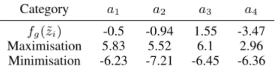
Table 6: Reponse for each Mel spectrogram in Figure 4.a1, a2, a3anda4refer to reponse values to

the corresponding noise vector.

Category a1 a2 a3 a4

fg(˜zi) -0.5 -0.94 1.55 -3.47

Maximisation 5.83 5.52 6.1 2.96