Predictive modelling of building energy consumption based on a hybrid nature-inspired optimization algorithm

Predictive Modelling of Building Energy Consumption based on

a Hybrid Nature-Inspired Optimization Algorithm

Shidrokh Goudarzi

_{, Mohammad Hossein Anisi}

_{*, Nazri Kama}

_,

_{Faiyaz Doctor}

_,

Seyed Ahmad Soleymani

_{, Arun Kumar Sangaiah}

a_{Advanced Informatics School, Universiti Teknologi Malaysia (UTM), Jalan Semarak, 54100 Kuala Lumpur, Malaysia} b_{School of Computer Science and Electronic Engineering, University of Essex, Colchester, CO4 3SQ, United Kingdom}

c_{Faculty of Computing, Universiti Teknologi Malaysia (UTM), Skudai, 81310, Johor, Malaysia}

d_{School of Computing Science and Engineering, Vellore Institute of Technology (VIT), Vellore-632014, Tamil Nadu, India}

Abstract- Overallenergy consumption has expanded over the previous decades because of rapid population, urbanization and industrial growth rates. The high demand for energy leads to higher cost per unit of energy, which, can impact on the running costs of commercial and residential dwellings. Hence, there is a need for more effective predictive techniques that can be used to measure and optimize energy usage of large arrays of connected Internet of Things (IoT) devices and control points that constitute modern built environments. In this paper, we propose a lightweight IoT framework for predicting energy usage at a localized level for optimal configuration of building-wide energy dissemination policies. Autoregressive Integrated Moving Average (ARIMA) as a statistical liner model could be used for this purpose; however, it is unable to model the dynamic nonlinear relationships in nonstationary fluctuating power consumption data. Therefore, we have developed an improved hybrid model based on the ARIMA, Support Vector Regression (SVRs) and Particle Swarm Optimization (PSO) to predict precision energy usage from supplied data. The proposed model is evaluated using power consumption data acquired from environmental actuator devices controlling a large functional space in a building. Results show that the proposed hybrid model out-performs other alternative techniques in forecasting power consumption. The approach is appropriate in building energy policy implementations due to its precise estimations of energy consumption and lightweight monitoring infrastructure which can lead to reducing the cost on energy consumption. Moreover, it provides an accurate tool to optimize the energy consumption strategies in wider built environments such as smart cities.

Keywords:Energy consumption, algorithm design, prediction.

1.Introduction

According to the International Energy Agency (IEA) [1], there will be a 30% increase in the global demand for electricity by 2040. This is in part due to population growth, increased accessibility to electricity through growing urbanization and an increasing population living in urban centres within developing and emerging economies [2]. With urbanization comes the need to build more power-hungry infrastructures in the form of new homes, community centres, workplaces, hospitals and schools. The UNEP express that buildings contribute to 33 percent of the energy produce and account for around 20 percent of carbon dioxide and other greenhouse gas emissions globally [3]. A recent UN Environment report has further warned that energy inefficient buildings could prevent us from reaching the target set by the Paris Climate Agreement of keeping keep global warming

* Corresponding author. School of Computer Science and Electronic Engineering, University of Essex, Colchester, CO4 3SQ, United Kingdom. E-mail address: [email protected]

below 2°C [4]. To meet these targets, the energy intensity of the global buildings sector needs to improve by 30 percent by 2030 according to The Global Alliance for Buildings and Constructions [4]. Although there have been improvements in the effectiveness of new buildings these efforts are not keeping pace with the remarkable extension of the world’s cities. As most new buildings will be built in developing countries, there is concern over the lack of standards and agreements for mandatory regulations for energy efficiency that must be complied. Additionally, there is a need to make energy efficiency provisions smarter, more accessible and affordable for monitoring and meeting the usage requirements of new and existing buildings. This is especially true for multifunctional community and religious buildings such as library building that tend to be functional throughout the day and night to serve a variety of purposes and usage needs.

Efficient management of the energy in smart building can be used to reduce the operational costs by assessing the amount of energy that end-users consume from lighting and electrical equipment and lowering the used amount for an individual or a group of end-users. Effective energy consumption management of inhabited spaces can be achieved by continuously monitoring the usage of electricity points and environmental control actuators to use this information to optimize the way electricity is consumed without compromising the utility and functionality of the space. However due to the huge number of possible actuators (fans, lights, HVAC, blinds, window actuators etc.) and electricity outlets within large and multifunctional user spaces there is both a need to develop effective infrastructures to sense and connect these devices together to capture data on energy usage as well as model and predict usage patterns for managing and optimizing the overall energy consumption of the building [5]. There has been an expanding growth in automated control frameworks and computational improvement methodologies applied to big data analytics [6] for modelling energy usage to provide accurate consumption estimations. Zhou et al. [7] has introduced an extensive vision for big-data-driven intelligent energy management through intelligent power generation, power transmission, power distribution and transformation, and demand side management. These big data drive applications can enable better energy estimation and management while considering the “4V” features of using large datasets that consider its volume, velocity, variety, and value [7].

Different machine learning and predictive modelling techniques have been included as part of energy management sensing and control frameworks. Regression analysis has conventionally been the most common approach in context of vehicle energy consumption prediction, solar energy prediction, and energy consumption prediction in buildings [8-12]. Artificial neural networks (ANNs) have also been adopted for predicting energy consumption where in [12] an ANN has been trained on data extracted from a simulation to draw a mapping between the input and output for anticipating energy consumption. In addition, decision trees have also been used in production systems as an efficient decision support technique to dynamically control changing industrial production processes [13].

In [14], both Genetic Algorithms (GA) and ANNs were utilized to forecast the electrical energy consumption and in [15] ANN, fuzzy systems and GA were used to find a buildings thermal response to variables including internal occupancy and building plant responses and outside weather conditions. A hybridization of fuzzy logic modelling and ANNs was introduced in [16] to perform long-term distribution prediction achieving a high accuracy based on extensive testing on actual data acquired from a small power distribution organization. In [17, 18] multiple regression analysis techniques have been adapted for the same purpose while in [19] an approach based on the decomposition method is described to explore diverse univariate-modelling procedures to provide estimation of monthly electric energy utilization in Lebanon. Univariate systems such as autoregressive, techniques combined with moving average and a novel structure from coordinating the pass filter with an autoregressive approach have also been presented in [20].

The Autoregressive Integrated Moving Average (ARIMA) [21] is a statistical liner model for time series prediction which has been shown to be suitable for modelling short-term forecasting and has been utilized in an assortment of applications such as predicting energy demand [21], wind speed forecasting [22], vehicular traffic

flow prediction [23] and sales forecasting [24]. The ARIMA model is a popular time series prediction model [25] and is well suited for monthly consumption [26] forecasting of energy usage. In the study by Pappas et al. [27], ARIMA is used for electricity consumption prediction and is shown to outperform other compared analytical time-series methods. Li and Hu in [28] developed a hybrid model for time-series prediction based on ARIMA and fuzzy systems. Here a fuzzy model is applied on data to determine fuzzy rules. The ARIMA model is hybridized with fuzzy rules. A key drawback of ARIMA is low accuracy in prediction of fluctuating or non-stationary time series data. Additionally, the symmetrical joint distribution of the static ARIMA method is unsuitable for data with strong dis-symmetry and the technique has been shown to be ineffective in adjusting the parameters of the method when the time series comprises new information. Also, the ARIMA model has limitation to capture and detect data features in linear and nonlinear domains. The most critical issue is lack of accurate data in forecasting field, therefore the hybrid model proposed in this study is composed of the ARIMA, SVR and PSO components. This enables the hybrid approach to model the linear and nonlinear patterns with improved overall predicting performance.

The main contribution of this study is in the development of a hybrid computational model for energy usage prediction. Here the ARIMA method is optimized by using a hybrid Support Vector Regression (SVR), Particle Swarm Optimization (PSO) for modelling linear and non-linear components in power consumption time series data for accurately forecasting power usage. False Nearest Neighbours (FNN) is used to pre-process the time series data to determine the minimum sufficient embedding dimension used to explicate the dynamics in the data. The SVR model’s hyper parameters are optimized using the PSO to improve prediction accuracy of the overall model.

The optimized hybrid ARIMA model is better able to handle non-stationary or fluctuating nature of power consumption data from different connected power appliances in the building. The proposed hybrid approach is computational efficient and simple to implement as part of an automated power monitoring system for forecasting and managing large scale building wide energy consumption. The prediction model forms the central element of a novel light weight IoT framework for localized energy consumption forecasting in large multi-functional building using a cost-effective remote sensing and embedded computing infrastructure. The approach is evaluated on real power consumption data of environmental actuator devices controlling a large library building containing several energy consuming devices. The performance of the proposed prediction method is evaluated using data obtained from a library study room equipped with environmental control actuators consisting of several lights, fans and air conditioners. The whole study room is zoned into three areas where the environmental actuators in each area are supplied through three separate power lines that are connected to a central control box. A current sensor is attached to each of the three power lines. A micro controller (Raspberry Pi) has been used to read the current and convert it to power (measured in kWs). This data is then transmitted to an IBM bluemix virtual server using 4G and recorded to a My SQL database. Using the above system, the power consumption of the study room was continuously monitored over a period of one month at a frequency of 1-minute intervals. Results showed that the new hybrid technique performs well in energy consumption prediction compared to non-optimized methods. The proposed prediction model can be used in various type of applications such as industrial automation, building automation systems, building safety application, cooling, heating, and power applications for intelligent building.

The rest of this paper is organized as follows. Technical background on the data preprocessing and prediction techniques used in this study are described in Section 2. The preprocessing approaches and main modeling process are presented in detail in Section 3. A performance comparison of the proposed approach with the state-of-the-art techniques is presented in Section 4. Conclusions can be found in Section 5.

2.Technology Background

Suganthi and Samuel in [29] have investigated many different computational forecasting techniques for the field of energy prediction where their study identifies traditional predicting methods such as econometrics models, time series, regression and ARIMA compared to computational intelligence methods such as genetic algorithm (GA), fuzzy logic, neural network, and support vector regression models. The study found that ARIMA methods can be effectively combined with soft computing strategies to enhance the precision of energy forecasting model. The work in [24] has also proposed the usage of an ARIMA technique for predicting Greek electricity utilization where the planned technique in comparison with three systematic time-series methods showed better results. time series model is further proposed in [30] for short term hourly prediction for peak loads using an improved ARIMA model where the prediction results show better results over the original model. Based on these and other studies it is therefore argued that new optimized ARIMA models can achieve good performance for longer-term, more stable data sets while also handling noisier, more volatile data.

Binary classification problems are addressed by Support Vector Machines (SVMs). To do that, they are formulated as convex optimization problems [31]. Such problem involves using the maximum margin to separate the hyperplane, and properly classifying maximum possible number of training points. SVMs are able to represent this optimal hyperplane with support vectors. A generalization of SVMs is Support Vector Regression (SVR) [32-35] which introduces an insensitive area surrounding the function that is names as ε-tube to extends SVMs. The optimization problem is re-formulated by this ε-tube to discover the ε-tube that is able to approximate the continuous-valued function appropriately. At the same time, the complexity of the model and the error of prediction should be balanced [36]. Hence, a convex ε-insensitive loss function is defined and minimized and the flattest tube containing maximum training instances to formulate SVR as an optimization problem. It constructs a multi-objective function from the tube’s loss function and geometrical properties. Suitable numerical optimization methods are able to solve a large variety of convex optimization. Support vectors represent the hyperplane as training samples outside the tube’s boundary [36]. The determination of hyperparameters is considered as a limitation of SVR that needs practitioner experience. Inappropriately selection of hyperparameter settings and kernel functions might result in considerably low performance [32-35]. The use of optimization algorithms such as genetic algorithm (GA) and chaotic genetic algorithm (CGA) have been employed to discover the optimal hyperparameters for SVMs [37, 38]. An approach for electricity load prediction has been presented in [17] and [39] that uses hybridization support vector regression schemes with simulated annealing (SA).

Compared with GA and simulated annealing (SA), Particle Swarm Optimization (PSO) is able to memorize the optimality of solutions (represented as particles in a swarm) over each iteration step. As all particles are able to remember the best position reached during the past iterations as well as share data over the swarm. As such PSO can achieve better performance in selected domains compared to other evolutionary optimization approaches.

In this study, we introduce a new optimized ARIMA method for monitoring and predicting energy consumption from various electrical building actuators towards optimizing inefficient power usage and reducing overall power consumption. The ARIMA model is used to generate residual vectors for estimating the linear components in pre-processed power consumption timeseries data. The residuals are embedded within a predefined dimension to construct out residual vectors constructed by the SVR that are then used to extract the nonlinear patterns for forecasting energy usage from supplied data. PSO is further used to discover the optimal hyperparameters for SVR to improve its prediction accuracy of the combined hybrid model.

The following subsection provide details of the ARIMA, SVR and PSO techniques used in the proposed hybrid method along with False Nearest Neighbors (FNN) data pre-processing techniques used to generate the datasets for the training and testing the proposed prediction method.

2.1.ARIMA Method for Prediction Operations

The ARIMA approach was presented as a prediction method by Box and Jenkins [40]. This method is based on a linear combination of past values (AR) and errors (MA), namely autoregressive integrated moving-average (ARIMA). ARIMA method is a linear technique that predicts the linear component. Non-linear techniques are also used to forecast the other elements in time series. In this study we used optimization techniques to design the best possible ARIMA-based method for predicting timeseries data. ARIMA methods involve one variate as they use only the history of the time series to show how the variables respond with previous random variant. ARIMA can be executed through the three steps after collecting historical data of the relevant parameters. These three stages are identification, estimation and diagnostic checking [40]. An exhaustive explanation of the ARIMA method is presented in [40, 41].

Formally, ARIMA (p, d, and q) comprise of the parameters p, d and q where, p is equal to the number of autoregressive (AR) terms, q shows the number of lagged moving averages (MA) and d is equal to the number of non-seasonal variances. The method uses to describe the time series expressed as follows:

( )∇ = ( ) (1)

where and denote energy consumption and error at random time t, consistently. B represents a regressive shift operator well-defined by = , and associated to∇; the order time of differencing is defined by d; ∇= 1 − B, ∇ = (1 − ) . (B) and (B) and are moving averages (MA) and auto regressive (AR) and operatives of orders and as follows:

( ) = 1 − − − ⋯ − (2)

( ) = 1 − − − ⋯ − (3)

where , , , …, are the autoregressive coefficients and , , , …, are defined as the moving average coefficients. Also, the time series is denoted as linear transfer function of the noise series:

= + ( ) (4)

( ) = 1 + + + ⋯ (5)

where ( ) can be computed as ( ) = ( )/ ( ).

To utilize ARIMA method, we need to fix the partial autocorrelation (PACF) and autocorrelation (ACF) functions. In addition, the means of the partial autocorrelation graph and the autocorrelation graph of data are used to compute the order of the AR and MA parameters.

As mentioned previously, to implement the ARIMA method three steps are taken. In the first step of model identification, data should be often stationary since it is extremely important in ARIMA forecasting. To stabilize variance in data, differencing is normally applied [41], and the parameter d is determined. For time series and probabilistic methods’ stationarity can also be identified referring to PACF and ACF. Parameter estimation is the second step where Akaike’s Information Criterion (AICC) [42,43] and Schwarz’s Bayesian Information Criterion (BIC) [41] are minimized through parameter estimation in which both AIC and BIC compute the maximum log likelihood of the model. BIC is structurally similar to AIC but includes a penalty term dependent on sample size. We achieved the results of ARIMA model by Eviews software. The non-stationary of data is shown as ascending data. We assigned 1 to parameter, to make a difference on data. According to data correlation with 1 lag, we considered 1 and 2 as predicted values for AR, it means that 1 and 2 refer to AR value

and, we computed 1, 2, and 3 as measured values for MA parameter. After comparison, we should recognise the best ARIMA model. In this purpose, two models [1, 1,2] and [2, 1, 1] have been selected as appropriate models. AIC and BIC criterions comparison for [1,1,2] and [2,1,1] ARIMA methods are shown in Table I. The best ARIMA model with low values is chosen. The [1,1,2] model with AR = 1 and MA = 2 is selected as superior ARIMA model.

TABLE I

AIC AND BIC CRITERIONS FOR ARIMA’S MODELS

ARIMA’S Model [2,1,1] [1,1,2]

AIC 8.663 8.326

BIC 8.797 8.529

In the last step of ARIMA method, the precision and the error stationarity of the model are evaluated. Some predictive error performance measures such as root mean square error (RMSE) and mean absolute error (MAE) are applied to select the best model [43].

The ARIMA method [ARMA (p, q)] can be defined for x time series which contains instances through forecasting equations (6), (7) as follows:

= + + (6)

= + ⋯ + + = + (7)

where ( ) shows the original data and ( ) shows the predicting data; the m-dimensional vector is uncorrected random data with zero-mean and covariance matrix R, = ( , ) refers to the order of the predictor where p presents the number of autoregressive terms, q refers to the number of lagged forecast errors in the forecasting equation and , … , and , … , are the × coefficient matrices of the multivariate (MV) ARMA method. The random errors ( ) are supposed to be self-determining and possess identical distribution with a constant variance. In this study the linear components of the energy consumption timeseries data acquired from the environmental sensors can be predicted using these equations.

2.2.Support vector regression

The SVR [44] used in this study is developed according to the structural risk minimization (SRM) principle that can minimize the upper bound of the generalization error. For the case of regression approximation, suppose there are a training set of data , where ∈ is th input data, is the th predicted output of , the number of training samples is shown by and embedding dimension is presented with . The main target of SVR is to detect the optimal function among other possible functions as follows:

= ( ) = ( ) + (8)

where ( ) is the high dimensional feature space, which is nonlinearly mapped from the input space x and b is a bias constant or threshold. W and b are estimated by minimizing the following optimization problem:

1

Minimize the regularized error is required to find the optimal function ( ), where > 0 is a regulatization factor, the 2-norm on function is ‖ ‖ and , ( ) is a loss function. Eq (8) is used to present the sparsity in SVR in the -insensitive loss function. This formula creates an ability for more forecasting to decrease within the boundaries of the −tube.

, ( ) = 0, | ( ) − | <_{| ( ) − | − , ℎ} (10) The SVR uses the nonlinear kernels to map samples into a complex dimensional space. The following form is the regression function:

( ) = ( − ∗_{) ( , ) + (11)}

where and ∗ _{are Lag range multipliers and ( , ) is a kernel function. We applied the Gaussian kernel} function of the form, ( , = exp ( )), where is a parameter of the Gaussian kernel.

2.3.Particle swarm optimization method

Particle swarm optimization (PSO) is an optimization nature-inspired algorithm [45] that works based on social behavior of bird flocking or swarming of insects or fish schooling [46]. In nature, the movement of a bird is adjusted to discover a better position in the flock based on the experience obtained by the bird and the neighboring birds. Nowadays, PSO has gained much attention in wide applications for solving continuous nonlinear optimization problems because of its simple concept, easy implementation and fast convergence [45]. For the optimization problem pertaining to this study, each particle represents as a suitable solution. Particles move in a k dimensional search space. Movement is performed by each particle constructed on prior knowledge and interactions with other particles in each iteration. All particles adjust their positions in the solution space towards being associated to the best solution (fitness criterion), which has been recognized thus far by these particles. This value is titled the personal best, pbest. PSO tackles another value that is the best value distance acquired subsequently by the particles. This is called, gbest. Basically, PSO focuses on the fast-tracking particles according to their pbest and gbest locations over each iteration. Each particle calculates its velocity to perform movements and then each particle can update its position for each iteration. The variation of the velocity of the particle is mathematically formed as follows:

( + 1) = × ( ) + × () ×

− ( ) + × () ×

− ( ) (12)

where ∈ [− , ], () is a random function which uniformly distributed random number between 0 and 1, the and are, respectively, related to weighting factors and denote the personal learning factor and social learning factor and is inertia factor. The following equation is designed to display the new solution:

2.4.False nearest neighbors (FNN)

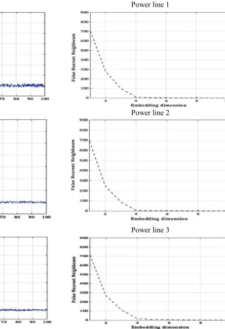
A significant step in time series analysis is the identification of the minimum (necessary) embedding dimension for reconstructing the dynamics in the data, where such information is either hidden or not known a priori [47]. If the embedding dimension is less than the actual dimension of the system, the computed models can be inaccurate as the dynamics in the data have not been completely unfolded. If, the embedding dimension is too large, the number of data points in the time series would be correspondingly large leading to excessive computation. This also increases computational error due to the presence of additional unwanted dimension where no dynamics are operating [47].

Selecting the embedding dimension is therefore very significant to predict the historical data. An effective technique of finding the minimal sufficient embedding dimension is the False Nearest Neighbors (FNN) procedure, which was proposed by Kennel et al. [48]. FNN is a nature-inspired algorithm based on geometric. When the regression vectors have sufficient data to predict upcoming output, the future output of the two regression vectors which are also close together in the regression space, will be near it. Whenever, not adequate terms to reform the dynamics of the system are available in the regression vector, some neighborhoods in the regression space will have an extensive range of related forthcoming results. Trajectories that are near with very diverse outputs can be assumed could be considered as false neighbors, because their proximity is due to the projection onto a space with a dimension too small to denote the dynamics of the system.

To clarify the mechanism of false nearest neighbors, firstly, the FNN assumes the embedded dimension is = 1; so, it evaluates how far single points are to their neighbors by calculating the distances between , and , ∀ ≠ . Therefore, the FNN for embedded dimension equal to two ( = 2) must compute distances between ( , , , ) and ( , , , ) where ∀ ≠ . Accordingly, the FNN will compute distances between ( , , … , , ) and ( , , … , , ) where ∀ ≠ . The false nearest neighbors is calculated as follows:

 For a point ( ) in the embedding space, we have to find a neighbor ( ) for which − < , where ‖… ‖ is the square norm and is a small constant usually not larger than the standard deviation over all the data.

 The equation 14 shows the normalized distance as that is between the points a(i) and a(j):

=_{‖ ( ) − ( )‖}− (14)

 If exceeds a given threshold then in dimension m, the point ( ) is defined as a false nearest neighbor. According to [47], = 15 has proven to be a good choice for most data sets.

Another issue is the correct estimation of the time delay . We can determine , by using the first minimum of mutual information (MI) function [48]. The MI functions quantitatively measure the mutual dependence of the two variables based on the probability theory and information theory as follows:

( ) = ( , ) log _{( ) (}( , )₎ (15)

where ( ) presents the probability density of while ( , ) donates the joint probability density of and .

3.Our Proposed Framework

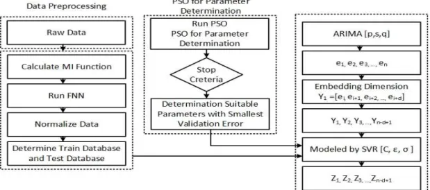
This section presents the proposed model including data pre-processing, the PSO algorithm for determining the SVM’s parameters and the proposed ARIMA and PSO-SVM model. The whole process is depicted in Fig. 1.

3.1.Data preprocessing

Initially, the MI function is computed using Eq, (15) to select the most relevant inputs for the power consumption dataset. In the second step, the first delay time is considered as the optimal time delay. This value is calculated using the MI function. In the third step the minimum sufficient embedding dimension are determined using the FNN approach. According to the optimal time delay and embedding dimension, the time series phase space is recreated to clear its hidden dynamics in the fourth step. Eq. (16) is used to normalize and fit the data in the interval (0, 1) in step five:

= −₋ (16)

Finally, in step six, two datasets, training and testing dataset are acquired by splitting the time series dataset. Here, we trained with 70% training data and tested on the remaining 30%. The data preprocessing procedure is illustrated in Fig.1.

Fig. 1. Flowchart of proposed model.

3.2.PSO for determine the SVR’s parameters

Good setting of hyper parameters , ε and the kernel parameters (σ) determine the prediction accuracy of the SVR. Parameter is specifies the tradeoff between the degree of the training errors larger than that are tolerated in Eq. (17) (i.e., the empirical risk) and the model flatness and. When has large boundary balue (infinity), the empirical should be decreased. Parameter ε is used to control the ε -insensitive zone’s width, for instance, the number of SVs used for the regression [42]. When ε –value is large, fewer SVs employed is implied; hence, the regression function is flatter (simpler). As mentioned previously there is no specific technique for effectively setting of SVR parameters.

In PSO, tracing and memorizing can be used to store each particle’s experience in searching process. As all particles can remember the best position they reached during the past iteration, the PSO process can hybrid self-experience search with neighboring self-experience search. In the traditional SVR technique the parameters were

selected using a grid search over a fixed interval of possible values for the parameters. In the hybrid PSO-SVR model, the PSO constructs a stochastic search for finding the best set of parameters of SVR. The position, velocity, and local best position of the ith particle pair can be defined as follows where these terms are defined based on the three hyper parameters in an SVR model for the n-dimensional space and are denoted in Eqs. (17)– (19), respectively,

( )

= [

,

,

, … ,

]

( )

= [

,

,

, … ,

]

( )

=

,

,

, … ,

, = , , , = 1,2, … ,

We initialize a population of particles ( , , ) with random positions ( , , ) and velocities ( , , ). Then, the global finest position between all particles in the swarm = [ , , , … , ] is shown as Eq. (20):

= [

,

,

, … ,

],

The new velocity of all particles in the population is then calculated by Eq. (21) as follows: ( )( + 1) = ( )( ) + (. ) − ( ) + (. ) − ( ) ,

= , , = 1,2,3, … , , (21)

where refers to the inertia weight which controls the impact of the prior velocity of the particle on its present one, where it is used to control the degree of exploration of the search, and are two positive constants. Rand (.) and rand (.) are uniform random variables with range [0, 1]. The new position of the particle for each parameter is determined in the next generation as follows,

( + 1) = ( ) + ( + 1), = , , = 1,2,3, … , (22) Notice that the value of each factor in ( ) is limited to the range [− , + ] to control excessive roaming of particles outside the feasible search space. This procedure is continued until a predefined threshold is reached. In this study, the forecasting error index, namely the mean absolute percentage error (MAPE) is used as the forecasting accuracy measure. The MAPE is used for measuring accuracy and is the criterion used for selecting the most appropriate parameters for usage in the SVR with PSO model, as shown in Eq. (23)

= ∑ × 100% (23)

where is the number of prediction periods, is the actual value at period and shows the predicting value at period . The smallest testing MAPE value is determined in the proposed model to be the most suitable model. The MAPE for testing of the three power lines are demonstrated in Table II.

TABLE II

MINIMUM TESTING MAPE VALUE

Power lines MAPE of testing (%)

Power line 1 1.4178

Power line 2 1.7001

Power line 3 1.3349

The PSO is employed to adjust the parameters with minimum validation error and select them as the most appropriate parameters.

3.3.Proposed ARIMA-PSO-SVR model

In this section we describe each phase of the proposed hybrid model which combines the SVR and PSO model components described in previous sections. In the first phase, the ARIMA (p, s, and q) model is used to estimate the linear component of the time series data which generates a where shows predicting data by ARIMA method (See, Eq. (7). The data are then embedded within a predefined dimension where a vector

= [ , , … , ] will be constructed by the SVR that can extract the nonlinear patterns.

In the second phase: the optimal hyper parameter set for SVR is determined using the PSO. The PSO determines the optimal set of parameters for the SVR comprising of the regression parameter ε, a constant C, and the kernel constant . In PSO, the search space is limited by min and max values of the parameters. In the third phase the final predictions will be based on the combination of predictions by the ARIMA and PSO-SVR models as follows:

= +  ₍₂₄₎

In the fourth phase, founded on the final prediction of the system, the fitness evaluation is computed. The mean square error (MSE) is used to measure the quality of prediction as shown in Eq. 25. Here a validation set is utilized to compute the suitability of a particle and test set is used to assess the performance of the system.

( ) = ∑ ( , ) ₍₂₅₎

4.Performance Evaluation

The performance evaluation of the proposed hybrid prediction method is based on data obtained from a library building in Universiti Teknologi Malaysia (UTM). Different data sets from a library building are collected to verify the forecasting ability of the proposed hybrid model. All data sets are derived from actual building energy usage data. Processing and transmission of data using a microcontroller (Raspberry Pi). Continuous energy monitoring system are used to monitor and detect unreasonable power consumption. Using the proposed system, the power consumption of the library building was continuously monitored over a period of one month at a frequency of 1-minute intervals.

In the advance of time series forecasting techniques, one of the significant steps is selecting the input data, which determines model’s structure [27]. In the data pre-processing step, we used MATLAB toolbox to compute MI function and FNN procedures. Figs. 2 and 3 shows the mutual function and FNN results for each dataset.

As energy consumption data has a number of non-stationary properties, diverse techniques need to be employed to modify the non-stationary attributes. The parameters of basic ARIMA method that are displayed

in Table III, are designed based on the Akaike Information Criterion (AIC) [49] that are used to measure of model performance based on the energy consumption data from three separate power lines. Previous experimental results over basic ARIMA method suggest that the predicting functions must be created by values shown in Table III

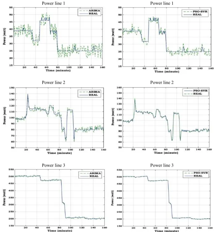
The comparative results of model fitting and forecasting for ARIMA against the real forecasting data on consumption for each of the three power lines are shown in Fig. 4, where the predicting data is organized from 101 to 120. The comparison of the basic ARIMA technique, the PSO-SVR-optimized model and the enhanced hybrid model against the forecasting data on consumption rates for each of the power lines are shown in Fig. 4 to Fig. 6.

We used the mean absolute error (MAE), the average relative error (ARE) and the square root of the mean

square error (RMSE) in order to evaluate the performance of the models on prediction accuracy. These evaluation measures are equated as follows:

where is the real value, and is the estimated value of . Tables IV to VI further shows the performance of each estimation model based on the predicted consumption of the three power lines supplying the library building compared to their forecasting data.

= ∑ ( − ) (26)

= ∑ | − | (27)

= ∑ (| − |⁄ ) (28)

TABLE III

ARIMA METHOD PARAMETERS OF THREE POINT-OF -USE.

ARIMA Power

line 1 Power line 2 Power line 3

p 3 5 3

d 3 1 1

q 1 0 0

TABLE IV

INDICES OF ARIMA METHOD.

Power

line 1 Power line 2 Power line 3

ARE 41% 40% 35%

MAE 1.2 0.9 0.89

RMSE 0.9 1.4 0.7

TABLE V

INDICES OF THE PSO-SVR METHOD.

Power line

1 Power line 2 Power line 3

ARE 39% 24% 22%

MAE 0.9 0.5 0.3

RMSE 0.7 1.1 0.5

TABLE VI

INDICES OF THE HYBRID METHOD.

Power line

1 Power line 2 Power line 3

ARE 27% 22% 21.5%

MAE 0.6 0.30 0.28

The power consumption prediction results of the ARIMA method shown in Table IV and Fig. 4 shows that the ARIMA method has the ability to explain the variation of the time series.

Though the basic ARIMA method has an efficient performance in the presence of energy consumption variation, the basic ARIMA’s predicting accuracy is not able to address the demand for energy storage in real-time electricity markets. To better predict the energy consumption, PSO-SVR was suggested to enhance the results

Power line 1 Power line 1

Power line 2 Power line 2

Power line 3 Power line 3

of the ARIMA method. For the three power lines, the PSO-SVR method optimizes the results of the ARIMA model and the predicting and predicting results have been presented in Fig. 5. In Figs. 4 to 6, similar trends to real data are observed in each model. However, there is greater differences notifiable between the real data and the results of basic ARIMA. The evaluation indices of the PSO-SVR-optimized ARIMA method are shown in Table V.

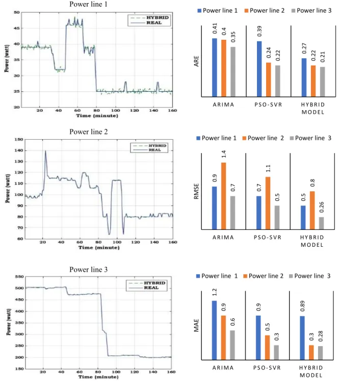
The optimized hybrid model that controls the forecasting error based on PSO-SVR-optimized ARIMA method for all three power lines, shows a significant enhancement for energy consumption prediction in the library building containing several energy consuming devices. The detailed indices are shown in Table VI. These results show an improvement of the hybrid model compared to both the basic ARIMA and PSO-SVR optimized ARIMA methods.

To assess the methods accurately, the performance indices of the different models over the three power lines are calculated and shown in Fig 7 according the measures defined above. From the results we see an improvement in the new hybrid optimized method regarding both the power consumption indices and forecasted results. For example, considering the ARE, in line 1, the values are between 41% and 22% for the basic ARIMA method and the PSO-SVR method but are decreased to 21% in the enhanced hybrid method.

In comparing the performance of the three approaches based on RMSE, for line 2 the value of the basic ARIMA method is 1.4575, while that of the PSO-SVR method is decreased to 1.1 and that of the optimized hybrid method is 0.8. Results of improved ARIMA with SVR and PSO are presented that RMSE, MAE and ARE criteria have been improved in PSO-SVR and new hybrid optimized method and overall acquires better results than non-optimized single ARIMA method. Also, SVR with PSO as an evolutionary algorithm is a viable alternative to improve the load forecasting accuracy successfully. As such, it can be used as a suitable method for energy consumption prediction. Overall Fig. 7 shows that the proposed hybrid model has the lowest RMSE, MAE, ARE evaluated on each of the three power lines. This suggests that the improved hybrid method can successfully reduce the error of the predicted values compared to the other two predicting approaches.

_{Power line 1 Power line 1}

Power line 2 Power line 2

Power line 3 Power line 3

Power line 1

Power line 2

Power line 3

Fig. 6. Predicting results of the optimized hybrid model. Fig. 7. Indices of different models in three point-of-use.

0. 41 0. 39 0. 27 0. 4 0. 24 0. 22 0. 35 0. 22 0. 21 A R I M A P S O - S V R H Y B RI D M O DE L AR E

Power line 1 Power line 2 Power line 3

0. 9 0. 7 0. 5 1. 4 1. 1 0. 8 0. 7 0. 5 0. 26 A R I M A P S O - S VR H Y BR I D M O DE L RM SE

Power line 1 Power line 2 Power line 3

1. 2 0. 9 0. 89 0. 9 0. 5 0. 3 0. 6 0. 3 0. 28 A R I M A P S O- S VR H Y B R I D M O DE L M AE

The performance comparison of proposed models on MAPE is stated in Table VII. The average error of proposed hybrid model, PSO-SVR and ARIMA for MAPE are 0.044962, 0.048743 and 0.050376 respectively and the hybrid model is graded first. The results of MAPE show that the hybrid model is more robust than other models.

TABLE VII

MODELS’ PERFORMANCE UNDER MAPE.

Model Power line 1 Power line 2 Power line 3

ARIMA 0.047765 0.049032 0.054331

PSO-SVR 0.046997 0.047145 0.052088

HYBRID MODEL 0.043495 0.044487 0.046906

Additionally, to prove the significance of accuracy improvement of the proposed hybrid model, a statistical t-test was conducted. Paired t-tests were performed separately for three power lines. The t-tests examine the performance of each model based on obtained results. A complete description for the t-tests is explained in [28]. We used the results of each model to compute the t-test statistic, that is, the ratio of the estimate of the magnitude of the slope to its standard deviation. We then calculate the p-value for each t-test on three power lines datasets where the results of this analysis are shown in Table VIII. The tests are obtained at a significance level of 95%. For this purpose, the significance effects have been set as effects with p-values, 0.05. It specifies models that vary considerably in accuracy.

TABLE VIII

P-VALUES FOR PAIRED T-TESTS.

Model PSO-SVR ARIMA

Power line 1 HYBRID MODEL 0.007 0.011 PSO-SVR - 0.182 ARIMA 0.299 - Power line 2 HYBRID MODEL 0.013 0.005 PSO-SVR - 0.243 ARIMA 0.154 - Power line 3 HYBRID MODEL 0.003 0.009 PSO-SVR - 0.315 ARIMA 0.108 -

According to Table. VIII, we can see that our hybrid model has outperformed other models based on a significant level of 95%. There is no high variance between other models. The ARIMA model is highly different from our proposed hybrid model. Overall, according to MAPE measurement, we can see that our hybrid model performs well in terms of prediction accuracy.

In this study, based on several applied methods, it can be supposed that combining linear and nonlinear methods with an optimization framework can demonstrate acceptable results with greater correctness, particularly when both methods offer good predicting strength.

5.Conclusion

In this work, an efficient hybrid prediction mechanism based on PSO-SVR and ARIMA has been proposed for accurate prediction of power consumption of actuation units in intelligent building environments. The main contribution of our prediction model is the hybridization of ARIMA model with an optimized PSO algorithm. In this study, we tried to show impact of PSO-SVR on optimizing parameters. The performance of the optimized hybrid method was assessed on monitored power consumption data of actuator devices from three zones that separately controlled the environment of a library building. The results indicated that the prediction and forecasting ability of new hybrid technique was able to out-perform the existing optimized SVR and the basic non-optimized ARIMA method.

These results show that the new hybrid model is a valuable method of planning and optimizing the ARIMA method in energy consumption prediction under real data. The new hybrid predictive modeling techniques offers several benefits. Firstly, the FNN is able to find the minimum sufficient embedding dimension in the time series data. Secondly, the proposed ARIMA method that is optimized by the PSO-SVR enables to model parameters to optimally adjust when dealing with non-stationary or fluctuating time series data used in predicting energy consumption; The merging of PSO-SVR with ARIMA provides an optimized hybrid method that has achieved consistently better prediction accuracies as has been shown from experimental results based on monitoring different combinations of building control devices powered using three different power lines. The ARIMA combined with PSO-SVR shows more advantages in terms of its computational efficiency. The method proposed in this study is also relatively easy to implement and deploy in different inhabited and functional spaces. More broadly the method can be extremely beneficial as an accurate tool to predict large scale building wide energy consumption that contribute to global energy consumption issues.

The main goal of this system is to streamline power management, monitoring and prediction into one single system such that inefficient power usage on various electrical appliances can be minimized to save on rising power utility costs. There can be various advantages and benefits from implementing such a system, the most obvious being that the cost of energy consumption can be significantly reduced. Moreover, the mobile aspect of our application using Raspberry Pi’s as our core architecture, provides scalability, processing power and a lightweight form factor for each device node that can be accommodated in a small and portable application and easily retrofitted to complement existing building management systems.

References

[1] Conti, J., Holtberg, P., Diefenderfer, J., LaRose, A., Turnure, J. T., & Westfall, L. (2016). International energy outlook 2016 with projections to 2040 (No. DOE/EIA-0484 (2016)). USDOE Energy Information Administration (EIA), Washington, DC (United States). Office of Energy Analysis.

[2] “World Health Organization (WHO) Background Guide 2015.” [Online]. Available: http://www.who.int/gho/urban_health/situation_trends/urban_population_growth_text/en/. [Accessed: 19-Jan-2018].

[3] H. Wang and P. Mancarella, “Towards sustainable urban energy systems: High resolution modelling of electricity and heat demand profiles,” 2016 IEEE International Conference on Power System Technology (POWERCON), 2016.

[4] “Power hungry buildings may jeopardize the Paris Agreement,” Futurism, 15-Dec-2017. [Online]. Available: https://futurism.com/power-hungry-buildings-paris-agreement/. [Accessed: 19-Jan-2018].

[5] H. Hani, I. Packharn, Y. Vanderstockt, N. McNulty, A. Vadher, and F. Doctor. "An intelligent agent based approach for energy management in commercial buildings." In Fuzzy Systems, 2008. FUZZ-IEEE 2008.(IEEE World Congress on Computational Intelligence). IEEE International Conference on, pp. 156-162. IEEE, 2008.

[6] I. Rahat, F. Doctor, B. More, Sh. Mahmud, and U. Yousuf. "Big data analytics: Computational intelligence techniques and application areas." Technological Forecasting and Social Change, 2018.

[7] K. Zhou, C. Fu, and S. Yang, “Big data driven smart energy management: From big data to big insights,” Renewable and Sustainable Energy Reviews, vol. 56, pp. 215–225, 2016.

[8] M. Dayarathna, Y. Wen, and R. Fan, “Data Center Energy Consumption Modeling: A Survey,” IEEE Communications Surveys & Tutorials, vol. 18, no. 1, pp. 732–794, 2016.

[9] S. B. Taieb, R. Huser, R. J. Hyndman, and M. G. Genton, “Forecasting Uncertainty in Electricity Smart Meter Data by Boosting Additive Quantile Regression,” IEEE Transactions on Smart Grid, vol. 7, no. 5, pp. 2448–2455, 2016.

[10] C.-M. Tseng and C.-K. Chau, “Personalized Prediction of Vehicle Energy Consumption Based on Participatory Sensing,” IEEE Transactions on Intelligent Transportation Systems, vol. 18, no. 11, pp. 3103–3113, 2017.

[11] B. Yuce and Y. Rezgui, “An ANN-GA Semantic Rule-Based System to Reduce the Gap Between Predicted and Actual Energy Consumption in Buildings,” IEEE Transactions on Automation Science and Engineering, vol. 14, no. 3, pp. 1351–1363, 2017. [12] S. A. Kalogirou, “Artificial Neural Networks and Genetic Algorithms for the Modeling, Simulation, and Performance Prediction of

Solar Energy Systems,” Assessment and Simulation Tools for Sustainable Energy Systems Green Energy and Technology, pp. 225– 245, 2013.

[13] W. Müller and E. Wiederhold, “Applying decision tree methodology for rules extraction under cognitive constraints,” European Journal of Operational Research, vol. 136, no. 2, pp. 282–289, 2002.

[14] T. Fei, F. Ying, Z. Lin, and L.T. W,” CLPS-GA: A case library and Pareto solution-based hybrid genetic algorithm for energy-aware cloud service scheduling,” Applied Soft Computing, vol. 19, 264-279.2014.

[15] Wang, Shuqing, Zipeng Zhang, and Liqin Xue. "Knowledge acquisition of fuzzy control system based on improved genetic algorithm and neural networks." In Fuzzy Systems and Knowledge Discovery, 2008. FSKD'08. Fifth International Conference on, vol. 5, pp. 95-99. IEEE, 2008.

[16] K. Padmakumari, K. Mohandas, and S. Thiruvengadam, “Long term distribution demand forecasting using neuro fuzzy computations,” International Journal of Electrical Power & Energy Systems, vol. 21, no. 5, pp. 315–322, 1999.

[17] Z. Mohamed and P. Bodger, “Forecasting electricity consumption in New Zealand using economic and demographic variables,” Energy, vol. 30, no. 10, pp. 1833–1843, 2005.

[18] C.-C. Hsu and C.-Y. Chen, “Regional load forecasting in Taiwan––applications of artificial neural networks,” Energy Conversion and Management, vol. 44, no. 12, pp. 1941–1949, 2003.

[19] S. Saab, E. Badr, and G. Nasr, “Univariate modeling and forecasting of energy consumption: the case of electricity in Lebanon,” Energy, vol. 26, no. 1, pp. 1–14, 2001.

[20] G. K. Tso and K. K. Yau, “Predicting electricity energy consumption: A comparison of regression analysis, decision tree and neural networks,” Energy, vol. 32, no. 9, pp. 1761–1768, 2007.

[21] V. Ediger and S. Akar, "ARIMA forecasting of primary energy demand by fuel in Turkey", Energy Policy, vol. 35, no. 3, pp. 1701-1708, 2007.

[22] R. Kavasseri and K. Seetharaman, "Day-ahead wind speed forecasting using f-ARIMA models", Renewable Energy, vol. 34, no. 5, pp. 1388-1393, 2009.

[23] B. Williams and L. Hoel, "Modeling and Forecasting Vehicular Traffic Flow as a Seasonal ARIMA Process: Theoretical Basis and Empirical Results", Journal of Transportation Engineering, vol. 129, no. 6, pp. 664-672, 2003.

[24] T. Van Calster, B. Baesens and W. Lemahieu, "ProfARIMA: A profit-driven order identification algorithm for ARIMA models in sales forecasting", Applied Soft Computing, 2017.

[25] Zhang GP. Time series forecasting using a hybrid ARIMA and neural network model. Neurocomputing 2003;50:159–75. [26] E. de Oliveira and F. Cyrino Oliveira, "Forecasting mid-long term electric energy consumption through bagging ARIMA and

exponential smoothing methods", Energy, vol. 144, pp. 776-788, 2018.

[27] Pappas SS, Ekonomou L, Karamousantas DC, Chatzarakis G, Katsikas S, Liatsis P.Electricity demand loads modeling using AutoRegressive Moving Average (ARMA) models. Energy 2008;33:1353–60.

[28] Li C, Hu J-W. A new ARIMA-based neuro-fuzzy approach and swarm intelligence for time series forecasting. Eng Appl Artif Intell 2012;25:295–308.

[29] L. Suganthi and A. A. Samuel, “Energy models for demand forecasting—A review,” Renewable and Sustainable Energy Reviews, vol. 16, no. 2, pp. 1223–1240, 2012.

[30] N. Amjady, “Short-term hourly load forecasting using time-series modeling with peak load estimation capability,” IEEE Transactions on Power Systems, vol. 16, no. 4, pp. 798–805, 2001.

[31] V. Vladimir. Statistical learning theory. 1998. Vol. 3. Wiley, New York, 1998.

[32] C.Y. Yeh, C.W. Huang, S.J. Lee, A multiple-kernel support vector regression approach for stock market price forecasting, Expert Systems with Applications 38 (2011) 2177–2186.

[33] O. Chapelle, V. Vapnik, O. Bousquet, S. Mukherjee, Choosing multiple parameters for support vector machines, Machine Learning 46 (2002) 131–159.

[34] K. Duan, S. Keerthi, A.N. Poo, Evaluation of simple performance measures for tuning SVM hyperparameters, Neurocomputing 51 (2003) 41–59.

[35] J.T.Y. Kwok, The evidence framework applied to support vector machines, IEEE Transactions on Neural Networks 11 (2000) 1162– 1173.

[36] A. Mariette, and R. Khanna. Efficient learning machines: theories, concepts, and applications for engineers and system designers. Apress, 2015.

[37] G. Jirong, Z. Mingcang, J. Liuguangyan, Housing price forecasting based on genetic algorithm and support vector regression, Expert Systems with Applications 38 (2010) 3383–3386.

[38] C.F. Huang, A hybrid stock selection model using genetic algorithms and support vector regression, Applied Soft Computing 12 (2012) 807–818.

[39] J. Sun, “Energy demand in the fifteen European Union countries by 2010 —,” Energy, vol. 26, no. 6, pp. 549–560, 2001.

[40] S. Barak and S. S. Sadegh, “Forecasting energy consumption using ensemble ARIMA–ANFIS hybrid algorithm,” International Journal of Electrical Power & Energy Systems, vol. 82, pp. 92–104, 2016.

[41] Z. Zhou, F. Xiong, B. Huang, C. Xu, R. Jiao, B. Liao, Z. Yin, and J. Li, “Game-Theoretical Energy Management for Energy Internet With Big Data-Based Renewable Power Forecasting,” IEEE Access, vol. 5, pp. 5731–5746, 2017.

[42] S. Goudarzi, W. H. Hassan, M. H. Anisi, S. A. Soleymani, and P. Shabanzadeh, “A Novel Model on Curve Fitting and Particle Swarm Optimization for Vertical Handover in Heterogeneous Wireless Networks,” Mathematical Problems in Engineering, vol. 2015, pp. 1–16, 2015.

[43] M. Drton and M. Plummer, “A Bayesian information criterion for singular models,” Journal of the Royal Statistical Society: Series B (Statistical Methodology), vol. 79, no. 2, pp. 323–380, Jul. 2017.

[44] V. Vapnik, The nature of statistical learning theory. springer, 2000.

[45] Kennedy J, Eberhart R (1995) Particle swarm optimization. Proceedings of the International Conference on Neural Networks: 1942– 1948.

[46] Vicsek T, Cziro´k A, Ben-Jacob E, Cohen I, Shochet O (1995) Novel type of phase transition in a system of self-driven particles. Physical Review Letters 75:1226–1229.

[47] Harikrishnan, K. P., Rinku Jacob, R. Misra, and G. Ambika. "Determining the minimum embedding dimension for state space reconstruction through recurrence networks." arXiv preprint arXiv:1704.08585, 2017.

[48] Kennel M B, Brown R, Abarbanel H D I. Determining embedding dimension for phase-space reconstruction using a geometrical construction. Phys. Rev. A 1992;45:3403–1.

[49] P. Sen, M. Roy, and P. Pal, “Application of ARIMA for forecasting energy consumption and GHG emission: A case study of an Indian pig iron manufacturing organization,” Energy, vol. 116, pp. 1031–1038, 2016.