Financial Wealth, Consumption Smoothing, and Income Shocks due to Job Loss

Income Shocks due to Job Loss

* _{Free University Amsterdam, Department of Economics, De Boelelaan 1105, 1081 HV Amsterdam,}

The Netherlands. Phone: + 31 20 4446037. Fax: +31 20 4446005. Email: hbloemen@feweb.vu.nl.

** _{OFCE, Sciences-Po, 69 Quay d’Orsay, 75007 Paris, France}

***_{This research project was started as part of the Tilburg TMR project on savings. The authors thank}

participants of the TMR-Workshop on Savings and Pensions (Paris, 2000), as well as participants of the Workshop on Applied Microeconometrics (Tinbergen Institute, Amsterdam 2001) for their comments. The authors are especially grateful to John Micklewright for having made the data available and to two anonymous referees for their comments. All errors are ours.

One of the reasons for setting up an unemployment insurance scheme is to allow job losers to smooth consumption. However, very little is known to date on the consumption smoothing impact of unemployment benefits. Here, we test for the impact of unemploy-ment benefits on changes in household food expenditure of individuals that have recently experienced a job loss, allowing for different levels of household’s financial wealth. We also study the relationship between unemployment benefits and financial wealth of the unemployed. We use for the empirical analysis a unique dataset rich on information on financial assets and debt of the unemployed. We conclude that there is significant hetero-geneity in the consumption responses of job losers to the income shock. For households without financial wealth at the time of job loss, unemployment benefits help smoothing food consumption. The results of estimation also suggest considerable heterogeneity in the relationship between borrowing and the level of benefits. For households running debt before job loss, there is evidence that higher replacement rates lead to postponing of paying off debt.

Keywords: Unemployment, Savings.

1

Introduction

The literature on consumption has generally ignored the potential impact of unem-ployment benefits on consumption smoothing of the unemployed. According to the life cycle theory, an expected income shock will not influence the level of consumption, as individuals will have accumulated a sufficient level of financial wealth and will run down their assets or will borrow if their level of assets is not sufficiently high. The underly-ing assumption is that individuals are not subject to borrowunderly-ing constraints. However, job losers are bound to experience borrowing constraints in reality. For example, credit institutions typically use the individual’s labour market status as a screening device for providing loans. The empirical literature on unemployment benefits has not paid much attention to the consumption behaviour of the unemployed either.1 _{This in spite of the} fact that income shedding motives are a rationale for providing unemployment insurance. Gruber (1997) studied the role played by unemployment benefits in consumption smoothing of the unemployed, and concluded, using PSID data for the United States, that a fall of ten percent points in the replacement ratio leads to a decrease in average food expenditure of 2.5%. Browning and Crossley (2001) specified a theoretical model of the consumption behaviour of the unemployed, which they estimated using data on total consumption for an ‘inflow’ sample of Canadian job-losers. The authors find that a decrease of ten percentage points in the replacement ratio would result in a decrease in total expenditure of 0.8%.2 _{Browning and Crossley (2001) also found that the} replace-ment rate affects consumption only when households hold no assets. A related issue was raised by Gruber (2001) who concluded that a higher replacement rate leads to a smaller decrease in wealth. Hamermesh and Slesnick (1998), investigated the impact of

unem-1 _{The emphasis has always been on the incentive effects of unemployment benefits. More recently,}

empirical studies on the impact of wealth on labour market transitions have appeared, like Stancanelli (1999), Bloemen and Stancanelli (2001), and Bloemen (2002).

2_{This smaller estimate than the one found by Gruber (1997) may be due to differences in the datasets}

used for the estimation, although typically food expenditure is less responsive than total expenditure to income shocks. Gruber (1997) used data from the PSID to estimate his model, while Browning and Crossley (2001) used data drawn from a sample of Canadians, unemployed for over six months. See Gruber (2001) and Browning and Crossley (2001) for more comments on these differences.

ployment benefits on households’ well-being, concluding that unemployment insurance helps to keep the consumption level of households affected by job loss as high as that of other comparable households in the economy.

Here we expand on the existing literature, by providing a separate analysis for the impact of the income shock, respectively, on consumption smoothing, savings and debt behavior of an ‘inflow’ sample of job-losers. We make use of a unique dataset which collects information on income, financial assets, debt and (food) consumption, both at the individual and at the household level, at different points in time, before and after entry into unemployment. This is the ‘Survey of Living Standards during Unemployment (LSUS)’.

The approach followed to model the consumption behaviour of the unemployed is similar to that put forward by Gruber (1997) and Browning and Crossley (2001). We measure the income shock that accompanies the job loss by means of the replacement ratio and we estimate its impact on the level of consumption measured just before job loss and three months after. The life cycle theory provides a natural link between the negative income shock and changes in consumption on the one hand and changes in wealth and debt on the other hand. If the household manages to smooth consumption by running down financial wealth, the income shock affects the level of financial wealth from one period to another but consumption is smoothed. If the household’s stock of wealth is not sufficiently high, the household may want to borrow and may well run into borrowing constraints. While running debt maybe subject to borrowing constraints and restrictions to access credit, cumulating assets should be entirely up to the individual. Here, we allow for a differential impact of the replacement ratio on savings and debt behaviour, by estimating separate models for the changes in financial wealth and debt.

Food expenditure data, used for our analysis, are supposedly less sensitive to an income shock than total consumption expenditure. Individuals experiencing an income shock may cut more substantially on durable expenditure than on food expenditure. For example, they may postpone to buy new clothes or to replace furniture. Browning and Crossley

(2000) deal with this topic extensively.

The structure of the paper is as follows. The next section lays out the theoretical background. The main feature of the data and some exploratory analysis of changes in consumption, financial wealth and debt holdings are presented in Section 3. Results of estimation of the relationship between unemployment benefits and consumption changes are discussed in Section 4. The relationship between changes in financial wealth and debt, respectively, and unemployment benefits is investigated in Section 5 of the paper. Section 6 summarizes the results of various sensitivity checks that were performed to test for the robustness of the empirical estimates. Conclusions are drawn in Section 7.

2

Theoretical background

The life cycle theory of consumption describes the consumption and saving behaviour of individuals that decide on the intertemporal allocation of income to consumption and savings. Assets accumulation and borrowing act as smoothing devices for intertemporal consumption. Uncertainty of future income is taken into account to model consump-tion patterns. In particular, to model the effect of an income shock due to job loss on consumption, the layoff probability can be incorporated into the model.3

Let the intratemporal utility function be denoted by u(ct, dt), which defines utility

in period t as a function of consumption in period t, ct, and the labour market state

occupied, dt (dt = 1 indicating employment, dt = 0 indicating unemployment). The

level of wealth at the beginning of period t is denoted by At. The interest rate and the

rate of time preference are denoted by rand ρrespectively. Wage income, unemployment benefits and other income are indicated bywt,btandµt.4 Thus, the intratemporal budget

constraint reads

ct+At+1 = (1 +r)At+dtwt+ (1−dt)bt+µt (1)

3 _{See, for instance, Blundell, Magnac and Meghir (1997).} 4_µ

tincludes the income of other household members. For the sake of exposition, it is assumed that the

income of other household members is not affected by the job loss of the individual under consideration. We relax this assumption later.

The objective of the individual is the maximization of the expected present value of utility, subject to the budget constraint (1). Blundell et al. (1997) show that the usual Euler equation for consumption remains valid if it is accounted for a layoff rate σt, which

defines the probability that a job loss materializes.5 _{Thus, for an individual, not subject} to liquidity constraints and employed in periodt, we may write

∂u(c1 t,1) ∂ct = 1 +r 1 +ρEt  (1−σ_t) ∂u(cd ∗ t+1 t+1 , d∗t+1) ∂ct+1 +σt ∂u(c0 t+1,0) ∂ct+1   (2)

The supercript for consumption indicates that the utility maximizing level of consumption will in general differ between labour market states, due to differences in income, and in (marginal) utility. The labour market state d∗_t+1 denotes the intertemporal utility maximizing labour market state in period t+ 1. The expectation operator in (2) refers to uncertainty in wages and other income.

The representation of the Euler equation (2) reveals the role of uncertainty in job loss on the individual’s behaviour. The average worker will have a job loss probability that is between zero and one and will save, accordingly, a certain amount every period. If a job loss materializes, the marginal utility of consumption receives a shock, both because of a change in the labour market state (the ‘permanent effect’) and because of the negative shock in income (the ‘benefit effect’). In the absence of liquidity constraints consumption is smoothed by saving or borrowing.6

The standard method of estimating an Euler equation is based on the recognition that the Euler equation establishes a moment condition. The moments are replaced by their sample counterparts and the model parameters may be estimated by GMM. If the sample is not selected on the basis of labour market movements, this is (under certain assumptions) a valid procedure, also in a model which includes uncertainty in the labour market state. In the present context, however, we are interested in the effect of an income

5_{Notice that the layoff rate may also be subject to uncertainty because, for example, of macro shocks}

to the economy. In the exposition we abstract from this type of uncertainty.

6 _{In the one extreme case in which the risk of job loss is zero, no additional savings will be made to}

prepare for the job loss, while in the other extreme in which the individual completely foresees the job loss, for example, if s/he has a fixed term appointment that comes to expiration, the expected income loss is anticipated and may be fully incorporated in the individual savings decision.

shock due to job loss on consumption, and for this purpose we use a sample of individuals experiencing a job loss. Browning and Crossley (2001) discuss this issue extensively. They show that the bias in the moment condition is equal to the permanent shock due to job loss. Their result is an important guideline for the empirical specification, since it suggests that in a regression framework for consumption changes covariates that are related to the permanent shock (i.e. to the change in marginal utility that may come from a change in labour market state) need to be included to serve as controls for the permanent shock to be able to measure the ‘pure’ consumption smoothing effect of the benefit. To this purpose one may include variables that account for previous job characteristics (earnings, tenure, industrial sector) and individual characteristics like age and family composition.

If liquidity constaints are present, the marginal utility of consumption will be affected by the benefit effect. In this respect, Browning and Crossley (2001) argue that the re-placement ratio affects consumption behaviour, and hence enters the regression equation, if households are liquidity constrained. In particular, asset holdings may be used as an indicator of liquidity constraints, but past earnings may also proxy liquidity constraints. The mirror image of consumption behaviour is saving and borrowing behaviour. Saving and borrowing are devices to smooth consumption. Unemployment insurance benefits provide job losers with an alternative or additional smoothing device. Thus, if households are able to smooth consumption completely by running down wealth, we would expect to find a significant impact of the replacement rate on household wealth. Running down wealth can be achieved by running down assets and by borrowing. A precautionary savings motive or liquidity constraints may weaken the possible relationship between the replacement rate and the saving behavior of households.

To make more explicit the relation between the income shock due to job loss on the one hand and the saving and borrowing behaviour on the other hand, we may write the budget constraint (1) as

∆At+1 = (rAt+dtwt+ (1−dt)bt+µt)−ct (3)

assets are run down, and/or borrowing takes place. The higher is the replacement rate, the lower will be the need to run down assets or to borrow. In the case of complete liquidity constraints, in which neither assets can be run down nor borrowing is possible, the left hand side of (3) is unaffected and consumption follows completely the income change. Thus, a relationship between the replacement rate and the change in wealth will be absent. In intermediate cases, in which individuals can run down assets, but not sufficiently to smooth consumption, or can borrow a little, the model predicts a weaker relationship between the replacement rate and changes in wealth than in the absence of liquidity constraints. Summarizing, the change in income due to a job loss is divided between a change in consumption and a change in wealth due to the adding up property implied by (3). How this division takes place depends on the extent to which the consumer is liquidity constrained. The precautionary savings motive may be an additional factor that affects this division.7

The theoretical model assumes the existence of perfect capital markets and therefore does not distinguish between saving and borrowing: borrowing is simply treated as nega-tive saving. However, individuals who wish to borrow may be subject to access limitations to the credit market, whereas assets accumulation is up to the individual. Access to debt may proxy liquidity constraints. Therefore, in the empirical analysis we look separately at the relationship between the benefit ratio, changes in the level of financial wealth and debt holdings.

The model presented describes individual consumption behaviour. However, in the data, consumption is observed at the household level and the unemployed in the sample are all household heads. The effect of the income shock experienced by the head of the household on the household’s consumption is likely to be smaller the larger are the other sources of household income. To account for this, Browning and Crossley (2001) use an ‘importance adjusted’ replacement ratio, which is given by the relative change in the unemployed’s earnings multiplied by the ‘importance’ of the head’s earnings (the ratio of

the head’s earnings before job loss to the total household income before job loss). This amounts to including the change in the head’s earnings relative to the total household income.8

3

The data used for the empirical analysis

We make use of a unique dataset which collects information on income, financial assets, debt and (food) consumption, both at the individual and at the household level, at different points in time, before and after entry into unemployment, for an ‘inflow’ sample of the unemployed. This is the ‘Survey of Living Standards during Unemployment (LSUS)’, collected in 1983-84, which is still about the only dataset useful for the purposes of our research, as it is extremely rich on information on financial wealth of the unemployed.9 Can the results of the analysis with the LSUS be generalized to hold at current times? At the time the LSUS survey was carried out, the underlying macro-economic situation was rather different as unemployment hit record levels in the UK. On the other hand, the unemployment benefit system was more or less the same than the one currently in place, at least for the first 6 months to one year of unemployment, and conditions of access to credit for the unemployed have not changed substantially.

The unemployed in the LSUS sample all started their observed unemployment spell in the summer of 1983, when they registered at mainland Great Britain unemployment ben-efit offices, from whose files the survey sample was drawn. A sample of benben-efit claimants

8 _{This procedure is grounded in the literature on household behaviour, from which it can be formally}

derived. The simplest model of household behaviour is the unitary model, which assumes one household utility function and pools together the income of all household members to determine consumption choices. In the collective model, on the other hand, the level of income of each household member contributes to determine their bargaining position within the household and may, therefore, have a separate effect on individual consumption. As information about consumption is available to us only at the household level, it is not possible to identify the unitary model from the collective model.

9 _{The British Household Panel Survey only collects information on individual assets and debt at one}

snapshot point in time, while the LSUS enables one to observe financial wealth before and after entry into unemployment. Moreover, the BHPS covers a population sample and therefore a stock sample of the unemployed rather than an inflow sample of the unemployed. As a consequence, the analysis of consumption smoothing and financial wealth accumulation of the unemployed using the BHPS would need to control for unemployment duration, which is not exogenous to the model. Moreover, the number of observations on unemployed will be much lower for a given wave, so only the pooling of many waves will lead to the same number of observations as LSUS.

with the following characteristics was interviewed: (i) household heads, i.e. married men or single people of either gender; (ii) aged between 20 and 58 years. Only those individuals that remained unemployed for about three months following the start of their unemploy-ment spell were interviewed. All the information in the survey is self-reported by the unemployed. The interviews were conducted personally by the interviewers at the homes of the survey participants. The first interview, conducted three months after the start of their (registered) unemployment spell, contained retrospective questions concerning the situation one month before the start of the unemployment spell.

For our analysis, we selected a subsample of individuals that reported to be employed attk; reported a positive amount of net earnings at tk; participated in the first interview

(at t1, three months after the loss of their jobs); reported positive benefit income at t1, and reported on (food) consumption levels, both at tk and t1. The unemployed reporting no benefit receipts were excluded from the sample as they may be misreporting benefits.10 Moreover, we excluded sample observations with a replacement ratio (based on earnings one month before the first interview and benefits at the first interview) of 200% or more, and observations with reported relative (food) consumpion changes that exceed 200%. Thus, we are left with a sample of 1315 observations.11

We use information on average weekly food expenditure, financial assets and debt of the unemployed at two different points in time: one month before the start of the unemployment spell (labelled timetk) and three months into the spell (labelled time t1). Individuals are unemployed for three months at t1. Changes in consumption, financial wealth and debts from tk to t1 are measured over a four-months period, three months of

10 _{Although registering at benefit offices as just starting an unemployment spell, which followed a job}

spell, they would not be entitled to either insurance or assistance benefits, three months into unemploy-ment. If they had exhausted their entitlement to UI, due to the “link spell rule” or they did not have enough contributions, they should still be able to claim SB benefits (see Stancanelli, 1994, for more details on this).

11 _{The total number of participants in the first survey is 2923. The number of individuals that reports}

to be employed attk is 1747, of which 1470 report a positive amount of earnings. Out of the sample of

individuals that report to be employed and report positive earnings, 1423 report positive benefit income att1. However, 13 observations show a replacement ratio of 2 or larger, and 14 report a relative change in

food consumption larger than 200%. Finally, for 88 observations, the relative change in food consumption fromtk tot1is not observed.

which cover a period of unemployment. Browning and Crossley (2001) use data from a Canadian inflow sample of individuals, unemployed for longer than six months. Gruber (1997) uses data from the PSID, selecting a sample of individuals that were currently unemployed but reported to be employed in the earlier wave.

Reported average weekly food consumption for the LSUS sample was 3125 pennies three months before entry into unemployment, attk, and 2511 pennies three months into

the unemployment spell, att1. Data from the Family Expenditure Survey (FES) for 1982, show that average weekly food consumption expenditure was equal to 3265 pennies for employed households and to 2545 for unemployed households. This validates the LSUS data on food consumption and supports our hypothesis of an income shock to the job losers in the sample.

Total financial wealth is obtained by adding up the amounts of assets reported in the following categories: (i) current account; (ii) deposit account; (iii) building societies, national savings and trustee savings accounts; (iv) stocks, bonds and other securities. Total debt includes the following types of debt holdings: (i) a loan with a bank or a finance house; (ii) an overdraft with a bank or credit card; (iii) any arrears with payments; (iv) money owed to friends or relatives. Total financial wealth and total debt holdings were computed adding up the asset and debt components (listed above) of both the head of the household and the spouse, when present. We control in the analysis for the receipt of redundancy or severance payments, which are paid at the end of the job which precedes the start of the unemployment spell. These payments are higher for jobs with higher wages and are a function of job tenure.12

The replacement ratio is constructed by dividing information on benefit income at t1 by the earnings at tk. The unemployment benefit variable is constructed as the sum

of receipts of Unemployment Insurance benefit (UI), which is conditional mainly on a sufficient contributions record, and Supplementary Benefit (SB), that is means-tested on

12 _{They are normally available only to those unemployed with previous employment spells longer than}

household’s resources.13 _{At the time of the LSUS survey, Unemployment Insurance} bene-fits were flat rate and SB benebene-fits could be claimed as from the start of the unemployment spell. Both UI and SB had additions for dependent spouse and children.14 _Housing ben-efits were not counted into the unemployment benefit variable but entered separately.15

Table 1 presents descriptive statistics for the sample. The percentage of women in the sample is relatively low (5.2%), due to the selection criterion of the sample (e.g. household heads). Most household heads (82.7%) report to be married at time t1. Furthermore, 32.2% of the respondents in our sample report to have no children, and 29% have children younger than six. The percentage of individuals that worked part time before job loss is 3.7%. In the five years preceding the survey, 45.3% had not experienced any spell of unemployment;16 _{25.1% had experienced one spell; 14% two spells and 15.6% more than} two spells. The survey includes information on the skill level and the industrial sector of the previous job. Accordingly, we distinguish three different skill levels. The highest skill level, which includes professional and intermediate workers, applies to 24.4% of the sample respondents. Skilled workers are the largest group, covering 45.5% of the sample, while the semi-skilled and unskilled worker (the lowest skill group) represent 30% of the sample. We compute five indicators for different industrial sectors, covering construction, chemistry and engineering, hotels and services, other manufacturing and other industries.

13 _{Ideally, one would like to have administrative information on benefit receipts. However, Stancanelli}

(1994) found that some consistency checks performed rather well. For example, she found that 71.2% of the unemployed that reported to receive unemployment insurance payments reported payments exactly equal to the official amounts, and 88.2% reported amounts that differed for less than£1 from the official figures.

14 _{Current unemployment benefits in the UK have a very similar structure, with the two benefit}

components, insurance (UI) and assistance (SB) merged into a single benefit payment, the jobseeker allowance.

15 _{Individuals could receive them also when in work. Until April 1983 housing benefit could be paid}

either together with SB benefits or separately by the local authorities. After April 1983, they were paid separately from SB by the local authorities.

3.1

Descriptives of the replacement ratio, consumption and

fi-nancial wealth variables

Table 2 contains sample statistics on consumption, wealth and income variables. The data show that 20% of the households receive a benefit of 2500 pennies per week, which corresponds to the flat rate UB. Over 75% of the observations receives a higher amount, and the empirical distribution does not show any obvious spikes above 2500 so it shows quite some variation in amounts. The mean benefit income is 4020 (with the median quite close to it), which is about 1.6 time the flat rate amount and roughly equal to the flat rate UB plus the UB addition for dependent spouse (1545 pennies per week). Individuals receive more than the flat rate benefits depending (non-linearly) on the number of children, the earnings of the spouse and the amount of wealth, measured at the start of the unemployment spell.

The average replacement ratio in the sample is 0.49. The data used by Gruber (1997) and Browning and Crossley (2001) cover completely exogenous sources of variation in the replacement rate: Gruber (1997) uses variation across states and across time, whereas Browning and Crossley (2001) exploit a change in the benefit system. Since our data covers a period of a few months, no such exogenous source of variation is available. Nevertheless, there is a great deal of variation in replacement rates due to the fact that benefits are partly means-tested, depend on the employment status of spouse, on the number of children and on the amount of contributions accumulated.17

To see how much weight the earnings of the head have in total household income, Table 2 also contains the ratio of the head’s earnings to the total household income attk.

The mean (median) value for this ratio is 0.82 (0.86). The 75% quantile shows a value of 1. Table 2 contains also information on other sources of household income. This includes the income of the spouse, and housing benefits.

A large difference is observed between the mean level of financial assets and the median level. This reflects the skewness of data on wealth. We observe the same for debt. We

17_{At the time of the LSUS two reduced flat rates, equal, respectively, to one half and two thirds of the}

observe a fall in food consumption after inception of the unemployment spell. The mean food consumption at t1, three months after entry into unemployment, is lower than the mean food consumption at tk, one month before unemployment. The same is true for all

the quantiles considered of the distribution of food consumption.

Table 3 illustrates relative food consumption changes. The mean and median relative change show a decrease in food expenditure of 17% following the job loss of the house-hold head. Changes in consumption for two subsamples are reported: (i) the subsample of households that reported positive financial wealth (73.1%) and (ii) the subsample of households that did not receive redundancy or severance payments (72.2%). The per-centage of households reporting a decrease in consumption is smaller (56.3%) for the first subsample, which is consistent with the intuition that households with financial assets are better able to smooth consumption. Since only households reporting positive wealth can run down assets, this is the more interesting subgroup to look at to analyze the change in wealth: setting the subsample reporting positive wealth at time k equal to 100, the per-centage reporting positive wealth has dropped by almost 13% (to 87.3), three months into the unemployment spell. For households that do not receive redundancy payments nor severance pay (72.2% of the sample) the decrease in consumption is slightly larger than for the total sample. The percentage of households reporting a decrease in consumption is also larger for this subsample.

Finally, note that 37.4% of the households report no change in consumption. This could be due to the fact that (i) we look at food consumption, which may be relatively inelastic with respect to shocks in income, (ii) we are looking at a time lapse of four months, which may be too short to observe changes in consumption for some of the households and (iii) rounding errors of households that in their own experience did not change their consumption pattern. Browning and Crossley (2001) also found a peak at zero total consumption change, even though the period over which they measured the change in consumption is 6 months. It is interesting to note that in our sample the peak at zero is larger for the subsample of households that do report positive wealth and smaller

for households without end-of-job payments.

Table 3 shows that the mean level of financial assets increases, while the median level decreases. As some of the households report no financial wealth, we cannot compute the relative change in financial wealth, as we did for consumption. On the other hand, looking at changes in levels is difficult because of the large skewness of the distribution of the differences.18 Therefore, we shall consider the ‘pseudo relative change’, defined as ∆ ln(1 +At), the change in the logarithm of one plus the level of wealth.19 The sample

mean is -0.4. The percentage of respondents reporting positive financial wealth falls from tk to t1. Initially 73.5% of the total sample reports positive financial wealth. Three months after job loss, this percentage falls to 67.5.

For debt the sample mean of the ‘pseudo relative change’ is positive (0.48). Almost half of the households in the sample (48%) reports some positive debt at tk. There is a

clear increase in the number of households running debt three months after the job loss: at t1, 58.4% of the households report some positive debt, which amounts to an increase of 10% points.

4

The impact of benefits on consumption smoothing

As shown earlier (Table 3), the unemployed in the sample experienced on average a decrease in food expenditure of 17%, with small differences for different subsamples of the unemployed. Here we estimate the relationship between the size of the income shock due to the job loss, measured by the replacement ratio, and the change in consumption. The replacement ratio (minus one) is weighted by the importance of the household head’s earnings relative to the total household income before job loss. The dependent variable is the relative change in consumption.

In order to estimate the ‘pure’ effect of unemployment benefits (measured by the replacement ratio) on consumption smoothing, it is important to account for factors that

18 _{The skewness for changes in wealth fromt}

k tot1 is 7.9.

19_{In the literature, the practice of transforming data on assets by adding one and taking the logarithm}

to correct for the scale effects, has been applied quite often. An alternative transformation is the inverse hyperbolic sine, see Burbidge, Magee and Robb (1988).

may influence the marginal utility of consumption in the different labour market states and the lay-off rate, as argued in Section 2. Therefore, we include in the empirical regression variables that are related to the previous job, such as the net earnings before job loss, the skill level, the industrial sector and a dummy variable indicating whether the job was part-time. To measure the labour force attachment of the individual we use information on previous experiences of unemployment in the five years preceding the observed unemployment spell. We would expect this indicator to be inversely related to the lay-off rate, so that individuals that were not unemployed in the past five years may experience a larger fall in consumption. On the other hand, past unemployment may reduce the level of assets. We account for demographic characteristics and household composition variables. We include a dummy for the employment status of the spouse in the year before the job loss of the head. One may also want to include lagged wealth and debt as they capture the financial situation of the household before the job loss. However, these regressors may be correlated with the error term if there is time constant unoberved heterogeneity in, say, preferences.20

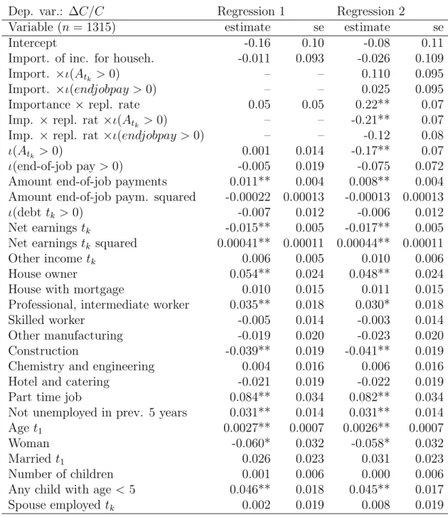
Table 4 contains the regression results. In regression 1, the importance of the head’s earnings in total household income before job loss and the replacement ratio weighted by this importance fraction show no significant effect on the relative change in consumption. We find a positive and decreasing effect for the amount of (lump-sum) end-of-job pay-ments: households which receive a larger amount of end-of-job payments experience on average a lower decrease in consumption. The dummies for positive wealth, positive debt and positive end-of-job payments do not show up significant. The level of net earnings before job loss is found to influence the consumption change negatively, but the marginal effect becomes smaller the larger is the level of net earnings.21

The dummy variable for house ownership without a mortgage is significant: job losers

20 _{We ran all regressions with and without lagged wealth and debt, variables and to find that they}

have hardly any effect on the sign of the coefficient on the replacement rate. In what follows, we present results of estimation without these regressors.

21 _{Higher order terms of net earnings did not have a significant effect on the relative change in}

who are house-owner outright, without a mortgage, experience a lower decrease in con-sumption than the other unemployed. House ownership with a mortgage does not appear to make a significant difference to consumption changes. Households with a head who had a part time job before job loss experience a significantly lower decrease in consumption. The difference between the marginal utility of working part time and the marginal utility of not working at all is likely to be smaller than the difference between the marginal utility of working full time and that of not working. Therefore, the consumption shock can be expected to be smaller for those who worked part time. Households whose head was not unemployed in the past five years experience a lower decrease in consumption, suggesting that this variable captures ability to save. Age has a significant positive ef-fect on the relative change in consumption:22 _{the older is the job loser, the smaller is} the drop in consumption. Age may correlate positively with the financial position of the household. Furthermore, the older the head of the household, the harder it may be for the household to change existing consumption patterns. Finally, we see that the drop in food consumption is smaller for households with young children: this probably indicates that the presence of young children affects the marginal utility of consumption.

Regression 2 in Table 4 estimates a more flexible specification of the relation between changes in consumption and the replacement rate, which allows the impact of benefits on consumption to differ for households reporting a positive amount of assets and/or end-of-job payments, by including cross-effects of the replacement rate with these variables.23 The estimation results indicate that for households who report neither asset holdings nor receipts of end-of-job payments, there is a significantly positive relation between the replacement rate and the relative change in food consumption. For these households, a smaller replacement rate translates into a larger fall in food consumption after the job loss: a drop in the replacement rate of 10% leads, for a household where the head’s earnings

22 _{Age squared turned out not to be significant.}

23_{To make sure that the cross effects do not merely measure differences in the importance of the head’s}

earning in total household income between households with and without financial wealth (and with and without end-of-job payments), we also included cross-effects of the importance weights and these dummy variables.

are the only source of income, to a 2% fall in food expenditure.

This is a somewhat smaller effect than the 2.5% found by Gruber (1997), without distinguishing job losers by their financial situation. It is larger than the 1.3% estimate of the same effect found by Browning and Crossley (2001), for total expenditure and for households reporting no assets before job loss. However, at least qualitatively, the results from these different studies are comparable. In particular, our finding of an insignificant effect for all households might be explained by the much smaller proportion (27%) of households with no wealth in our dataset, than in the sample used by Browning and Crossley (2001) (66%).

5

The impact of benefits on wealth accumulation

be-haviour

The descriptive statistics given in Table 3 show that after entry into unemployment households run down assets. In particular, we observe that the percentage of households running debt increases. The life cycle model of consumption suggests that there is a relation between the size of the income shock and the degree to which households run down assets or borrow. However, a low level of wealth and/or borrowing constraints may impede this relationship. In this section, we analyse whether changes in asset levels and debt holdings are influenced by the size of the replacement rate.

5.1

Changes in financial wealth and the replacement rate

First, we regress the pseudo-relative change in wealth (from period tk to t1) on the re-placement ratio. For this purpurse we restrict the sample to households reporting positive wealth at tk.24,25 The analysis is to some extent comparable to Gruber (2001), who also

relates the logarithm of wealth to the replacement rate, using a regression framework, and

24 _{We do not exclude observations reporting zero wealth att}

1, once they entered unemployment. 25 _{We did an auxiliary Probit analysis to gain some insights into the characteristics of households}

reporting positive wealth. We found that the probability of reporting positive wealth is higher for the unemployed with higher earnings before job loss, a working spouse, fewer unemployment spells in the previous 5 years and a higher level of education.

excluding households reporting zero wealth.

We present results of estimation of our model in Table 5.26 _{The replacement rate does} not show a significant effect on the change in financial wealth. End-of-job payments have a (decreasing) positive effect on financial wealth, allowing households either to dissave less or to increase asset holdings. Age has a significantly positive impact, indicating that older individuals tend to dissave less. Similar findings apply to married people and to those that have not been unemployed in the past five years.

As an alternative for the OLS-regression, we ran an ordered probit regression (see Table 5), distinguishing three groups: households with an increase in financial wealth (31% of the households reporting positive financial wealth attk); households reporting no

change in financial wealth (13%); and households reporting a decrease in financial wealth (56%). The advantage of the ordered probit model is that it is much less sensitive to skewness and noisiness in the dependent variable. The replacement rate again shows no significant effect. Finally, we ran a median regression. This method of estimation is less sensitive to outliers than OLS. Again, we do not find a significant effect of the replacement rate on changes in financial wealth. The same result was found for a regression of changes in financial wealth levels, used as an alternative to the logarithmic transformation.

Various additional sensitivity checks were carried out. For example, we did a regression of changes in saving for the selective subsample of households which reported a decrease in financial wealth. No significant relation between the replacement rate and the decrease in financial wealth could be detected. We also made a distinction between households who reported to have used all their assets from periodtk tot127and households who decreased wealth holdings but not to zero, for which a significant relationship was perhaps more likely to be found. We ran separate regressions of changes in wealth holdings for either subgroup, and also we ran an ordered probit (comparable to the regression in Table 5),

26 _{We have also ran regressions which included (a polynomial in) the level of wealth and debt in the}

right hand side. For the same reason as for the consumption equation, we present results without these variables among the regressors. The qualitative result for the replacement rate effect is not affected by the inclusion or exclusion of these variables.

27 _{There are 122 of such households in the sample, representing 9.3% of the total sample, and 12.6%}

with individuals reporting a decrease in wealth holdings split up in the two subgroups. None of these proved significant.

The theory indicates that the replacement rate has a positive impact on the change in financial wealth if the amount of financial wealth available to the household is sufficiently high (see Section 2). The empirical finding of an insignificant relation may suggest that for most households in the sample the stock of financial wealth is relatively low. Indeed, we saw an increase in the percentage of households reporting no financial wealth after entry into unemployment (table 3). Besides, households may not want to decumulate wealth substantially if they have a precautionary savings motive: if households are risk averse and the length of their unemployment spell is uncertain, they will be more reluctant to decumulate wealth.

5.2

Borrowing, postponement of paying off debt, and the

re-placement rate

Here we regress changes in debt on the replacement ratio, to investigate the ability of households to respond to the income shock. First, we ran a regression (not shown in the table) with the pseudo relative change in debt as the dependent variable and for all house-holds in the sample. The coefficient estimate of the importance weighted replacement ratio did not show up significant, but we found that households reporting end-of-job payments experience, on average, a smaller increase in debt, house owners with a mortgage register an increase in debt higher than the average and households with a larger number of chil-dren experience, on average, a larger change in debt.28 _{Next, we ran a regression where} we allowed the effect of the replacement rate on changes in debt to differ for households (not) reporting debt before job loss. The results of estimation (not shown) indicate that for households running debt before job loss, the change in debt is smaller, the higher the replacement ratio, suggesting that households can postpone paying off debt, the higher is

28 _{The first of these significant results is in line with the results in Table 3. The second, signals easier}

access to credit thanks to house-ownership. The third, is consistent with the result of the consumption regression, which showed that households with more children decrease consumption less: increasing debt may be used to finance this smaller decrease.

their replacement rate. For households reporting no debt before job loss, no significant relationship could be detected. Then, we allowed the impact of the replacement rate on changes in debt to differ for households (not) reporting positive amounts of end-of-job payments, to find that the replacement rate has a significant impact on changes in debt only for households that received end-of-job payments -perhaps signalling some capacity to postpone paying off debt.

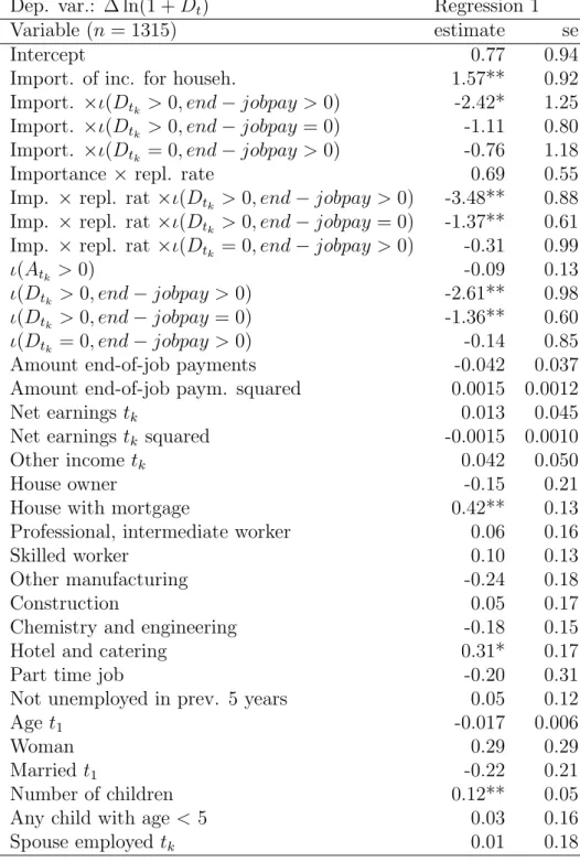
Our preferred regression, shown in Table 6, allows the effect of the replacement rate on changes in debt to vary for (i) households reporting positive end-of-job payments and debt before job loss, (ii) households not reporting any end-of-job payments but running debt before job loss, (iii) households reporting positive end-of-job payments but no debt before job loss and (iv) households not reporting any end-of-job payments nor debt before job loss (set as the reference group). For households of type (i) and (ii), we find that the replacement rate affects significantly the change in debt, a higher replacement rate leading to a smaller change in debt. In particular, the impact of the replacement rate on the change in debt is larger for households reporting some end-of-job payments. For households not reporting any end-of-job payments nor running debt before job loss, no effect of the replacement rate on changes in debt is found.

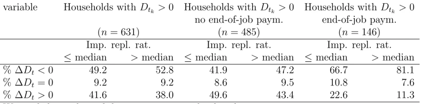
We ran some further tests to check whether the negative effect of the replacement ratio on the change in debt is due to households postponing to pay off debt or borrowing extra debt or a combination of the two. To this end, we split the subsample of households in debt attkinto households with a ‘low’ (smaller than the median) and with a ‘high’ (larger

than the median) value of the importance adjusted replacement rate and we looked at the distribution of changes in debt (see Table 7). Households with a ‘low’ replacement rate appear to be paying off debt relatively less often, and running up debt relatively more often, than households with a ‘high’ replacement rate. This result is more pronounced if we separate out households (not) reporting positive (any) end-of-job payments. There is evidence that households reporting positive end-of-job payments pay off debt relatively more often, but run up debt relatively less often than households not reporting any

end-of-job payments.

As an additional check, we ran two Tobit regressions: in the first, we censored the change in debt for values of zero and lower, implying that we concentrate on the analysis of increases in debt and in the second, we censored the change in debt for values of zero and higher (concentrating on decreases in debt, or, the paying off of debt). Table 8 displays the estimated coefficients on the replacement rate, which show that the results found earlier (table 6) carry over to the separate analysis of increases and decreases in debt. Therefore, we conclude that the negative effect of the replacement rate on changes in debt is due to households both paying off debt and running additional debt.

6

Sensitivity analysis

We ran some additional sensitivity analysis. For consumption changes we ran an ordered probit regression. As shown in Table 3, a number of respondents report no change in consumption from one month before unemployment to three months after. This may be due to rounding or recall error. The ordered probit explicitly accounts for the occurrence of a spike at the point of no change in consumption. It is also less sensitive to inaccuracies in the reported consumption values, since it uses interval-grouped consumption changes.29 We divided the change in relative consumption into five classes, according to the value of the relative change in consumption: (i) a positive value; (ii) zero value; (iii) negative but not lower than -25%; (iv) between -25% and -50%, (iv) between -50% and -75%; (v) lower than -75%. We included the same covariates as in regression 2 in Table 4. The results of estimation indicate that the qualitative conclusions are robust with respect to the method of estimation: all the covariates that have a significant impact in the OLS regression are significant in the ordered Probit and show the same sign.

So far the paper has not dealt with individual differences in expected unemployment duration. Households in a county with a high unemployment rate may expect the un-employment spell to last longer and be more careful in running down assets. Moveover,

29_{However, this decreased sensitivity may come at the loss of information due to the interval-grouping}

access to credit may be harder for the unemployed when the unemployment rate is higher. However, spacial differences in the level of unemployment may be stable over time, so that individuals in areas with higher (lower) unemployment than the rest of the country may (not) have anticipated the job loss and accumulated more (less) assets than the average. We re-ran the regressions for changes in consumption, financial wealth and debt, including the local rate of unemployment among the regressors. We found that the local unemploy-ment rate did not have a significant effect, neither in the model for consumption, nor in the models for financial wealth and debt.

We experimented alternatively with including a measure of the expected duration of the individual unemployment spell. Using the results of estimation of a hazard rate model of unemployment estimated on the same data (Stancanelli, 1999), we computed the predicted hazard rate of moving from unemployment into employment for the household heads in the sample and added it to the regressors.30 The coefficient estimate of the predicted hazard turned out not to be significant in any regression.

To test for the robustness of the estimates on financial wealth, we experimented with using an alternative measure of wealth that included only money held in a current account or a deposit account. This is a more restrictive, though more homogenous, measure of financial wealth. The qualitative results of the analysis of changes in financial wealth did not change either: no impact of the replacement rate on changes in financial wealth could be detected.

7

Conclusions

Allowing job losers to smooth consumption is one of the motivations for the existence of an unemployment insurance benefit system. However, until recently little empirical evidence on the consumption smoothing role of benefits was available. To shed light on

30 _{There are some identification problems with this approach as the same variables which are included}

in the consumption equations are also included in the hazard as the theory provides no exclusion re-strictions. Also, this extended model would imply that individuals can perfectly foresee the duration of their unemployment spell, which is an extreme assumption, under which individuals might also be able to smooth consumption completely.

the impact of unemployment benefits on consumption, the relationship between unem-ployment benefits and, respectively, financial wealth and debt holdings -which notably provide the unemployed with alternative instruments to smooth consumption- also de-serve attention. Liquidity constraints play an important role in the theoretical models that form the background for the empirical analysis.

We have modeled and estimated the effect of an income shock due to the job loss experienced by the head of the household on the household’s consumption, financial wealth and debt behaviour. In our model, the income shock is given by the decrease registered in the income of the household head as measured by the replacement ratio. The consumption variable is the household’s weekly food expenditure.

Using data on a sample of job-losers from the Survey of Living Standards during Unemployment, a longitudinal inflow sample of the unemployed in Great Britain, we find that the average household in our sample experienced a decrease in (food) consumption of 17%, three months into the unemployment spell. We find that following the job loss a smaller number of households reported positive amounts of financial assets and median household assets fell. Instead, the number of households running debt increased.

One could argue that the observed changes in consumption, financial wealth and debt may result from a downward macro-economic trend. However, a comparison of survey respondents over a longer period of time reveals that the consumption levels of job losers recover to the levels preceding the job loss for those re-entering employment, whereas they remain low for individuals who stay unemployed throughout the period. Furthermore, the income shock measured by the benefit replacement ratio is clearly specific to job losers. Information from the FES (1982) suggests that the observed change in consumption is consistent with a change in the labour market state.

If we do not allow for heterogeneity of household behaviour, no significant relation between the replacement rate and changes in food consumption is detected. If we allow the model to differ for households reporting a positive amount of financial wealth and households reporting no possession of any financial wealth, we find that households

re-porting no financial wealth experience a larger decrease in consumption the lower is their replacement rate. This is in line with the interpretation that households reporting no financial wealth are liquidity constrained, which adds to the role of unemployment bene-fits as a consumption smoothing instrument. Furthermore, it is possible that the income shock affects other components of the household total consumption function than food expenditure, which are not looked at in this study.

The quantitative implication of our analysis is that a decrease in the replacement rate of 10% results in a fall in food expenditure of 2%, for households reporting no financial wealth. Gruber (1997), who uses US data, finds a decrease of 2.5% in food consumption for all households in his sample. Browning and Crossley (2001) also found heterogene-ity between households reporting positive financial wealth and households reporting no financial wealth. They find that a cut in the replacement rate of 10% results in a 1.3% fall in total expenditures for households that report a zero amount of assets at job loss.

In addition, we find that households that receive (higher) end-of-job payments experi-ence a lower decrease in consumption. This provides evidexperi-ence that households use other financial resources to smooth (food) consumption, if they can afford it.

According to the theory, if households have a sufficiently high level of financial wealth, they will use it to smooth consumption in response to the downward income shock. Our empirical findings on the impact of the replacement rate on assets decumulation, suggest that either financial wealth is not sufficiently high or households are reluctant to use their financial wealth, as they have a precautionary savings motive and are uncertain about the length of their unemployment spell. On the other hand, we find evidence of heterogeneity in the relationship between the replacement rate and changes in debt. The results of estimation suggest that increases in debt result either from the postponement of paying off debt or from increased borrowing, the change in debt depending on the size of the replacement ratio. The finding of an insignificant relationship for households without debt before job loss may be explained by the binding of borrowing constraints.

References

Bloemen, H.G. and E.G.F. Stancanelli (2001), Individual wealth, reservation wages and transitions into employment, Journal of Labor Economics, Vol. 19, nr. 2. pp. 400-439.

Bloemen, H.G. (2002), The relation between wealth and labour market tran-sitions: an empirical study for the Netherlands, Journal of Applied Econo-metrics, Vol. 17, pp. 249-268.

Browning, M. and T. F. Crossley (2000), Luxuries are easier to postpone: a proof, Journal of Political Economy, Vol. 108, no. 5, pp. 1022–1026. Browning, M. and T. Crossley (2001), Unemployment Insurance Benefit Levels

and Consumption Changes, Journal of Public Economics, vol.80, pp. 1–23. Browning, M. and A. Lusardi (1996), Household Savings: Micro Theories and Micro Facts, The Journal of Economic Literature, vol. 34, pp. 1797–1855. Blundell, R. , T. Magnac and C. Meghir (1997), Savings and labour market transitions, Journal of Business and Economic Statistics, Vol. 15, nr. 2, pp. 153-164.

Burbidge, J.B., L. Magee and A. L. Robb (1988), Alternative transformations to handle extreme values of the dependent variable, Journal of the Americal Statistical Association, Vol. 83 (401), pp. 123-127.

Danforth, J. P. (1979), On the role of consumption and decreasing absolute risk aversion in the theory of job search, in: Lippman, S. A. and Mc Call, J. J. , Studies in the economics of search, North-Holland, Amsterdam. Fortin, B. and G. Lacroix (1997), A test of the unitary and collective models

of household labour supply, The Economic Journal, Vol. 107, no. 443, pp. 933-955.

insurance, American Economic Review, Vol. 87, no. 1, pp. 192–205. Gruber, J. (2001), The wealth of the unemployed, Industrial and Labor

Rela-tions Review, 55(1), October, pp. 79-94.

Hamermesh, D. S. and Slesnick, D.T. (1998), ”Unemployment Insurance and Household Welfare: Microeconomic Evidence 1980-93, ” in: L.J. Bassi and and S. A. Woodbury, Research in Employment Policy, Vol. I, Greenwich, JAI Press, pp. 33-61.

Stancanelli, E. G. F. (1994), The probability of leaving unemployment: some new evidence for Great Britain, PhD. thesis, European University Insti-tute, Florence.

Stancanelli, E. G. F. (1999), Do the rich stay unenployed longer? An empirical study for the UK, Oxford Bulleting of Economics and Statistics, vol. 61, pp. 295–314.

Table 1: Sample statistics: discrete background variables, sample percentages (n = 1315) Gender:

male 94.8%

female 5.2%

Marital status: (timet1)

married 82.7%

unmarried 17.3%

Houseownership and mortgage: (time tk)

houseowner without mortgage 8.1%

houseowner with mortgage 32.5%

renter 59.4%

Skill level:

professional, intermediate worker 24.5%

skilled worker 45.5%

semi-skilled/unskilled worker 30.0% Employment status spouse (time t1)

spouse employed 28.5%

spouse not employed 71.5%

Number of children (timet1)

no children 32.2%

one child 24.0%

two children 26.0%

more than two children 17.8%

Young children (time t1) (age< 5)

no young children 71.0%

young children 29.0%

Worked part time before job loss

part time 3.7% full time 96.3% Industrial sector other manufacturing 12.1% construction 16.3% chemistry engineering 24.9%

hotel and catering 15.8%

other industries 30.9%

# unemployment spells in past 5 years

Table 2: Sample statistics: The distribution of continuous variables

Variable mean quantiles

n= 1315 10% 25% 50% 75% 90% Savingstk £ 1411 0 0 121 700 2642 Savingst1 £ 2310 0 0 30 855 5002 debt tk £ 544 0 0 0 400 1100 debt t1 £ 532 0 0 60 400 1070 net wealth tk £ 867 -776 -170 4 500 5490 net wealth t1 £ 1778 -924 -263 0 701 4830

consumptiontk pennies weekly 3125 1500 2000 3000 4000 5000

consumptiont1 pennies weekly 2511 1200 1800 2500 3000 4000

age t1 38.6 24 28 37 49 55

Net earnings tk pennies weekly 9610 5400 6800 8500 11000 15000

Benefits t1 pennies weekly 4020 2500 2520 4045 4959 6150

replacement ratio 0.49 0.21 0.30 0.44 0.64 0.80

earnings head/total househ. inc. tk 0.82 0.57 0.70 0.86 1 1

Other income tk pennies weekly 2289 0 0 1350 3405 5646

Table 3: Observed relative changes in consumption, financial assets and debt

variable observation total positive no end-of-job

period sample savings payments

(n= 1315) (73.5%) (72.2%) Mean ∆Ct/Ct−1 Time K to 1 -0.17 -0.17 -0.19 Median ∆Ct/Ct−1 Time K to 1 -0.17 -0.17 -0.20 % with ∆Ct/Ct−1 <0 Time K to 1 58.6 56.3 63.0 % with ∆Ct/Ct−1 = 0 Time K to 1 37.4 40.1 32.7 % with ∆Ct/Ct−1 >0 Time K to 1 4.0 3.6 4.3

At: mean savings Time K 1411 1919 946

Time 1 2310 3078 1049

At: median savings Time K 121 306 61

Time 1 30 183 3

Sample % with At>0 Time K 73.5 100 68.3

Time 1 67.5 87.3 58.7

Mean ∆ ln(1 +At) Time K to 1 -0.40 -0.76 -0.93

% with ∆At<0 Time K to 1 41.2 56.0 46.5

% with ∆At= 0 Time K to 1 32.8 13.0 41.0

% with ∆At>0 Time K to 1 26.0 30.9 12.5

Dt: mean debt Time K 544 573 577

Time 1 532 558 635

Dt: median debt Time K 0 0 20

Time 1 60 50 105

Sample % with Dt>0 Time K 48.0 46.2 51.1

Time 1 58.4 55.7 65.6

mean ∆ ln(1 +Dt) Time K to 1 0.48 0.43 0.76

% with ∆Dt<0 Time K to 1 24.5 25.1 22.9

% with ∆Dt= 0 Time K to 1 42.2 44.6 37.0

Table 4: OLS regression for changes in consumption

Dep. var.: ∆C/C Regression 1 Regression 2

Variable (n = 1315) estimate se estimate se

Intercept -0.16 0.10 -0.08 0.11

Import. of inc. for househ. -0.011 0.093 -0.026 0.109

Import. ×ι(Atk >0) – – 0.110 0.095

Import. ×ι(endjobpay >0) – – 0.025 0.095

Importance × repl. rate 0.05 0.05 0.22** 0.07

Imp. ×repl. rat ×ι(Atk >0) – – -0.21** 0.07

Imp. ×repl. rat ×ι(endjobpay >0) – – -0.12 0.08

ι(Atk >0) 0.001 0.014 -0.17** 0.07

ι(end-of-job pay>0) -0.005 0.019 -0.075 0.072

Amount end-of-job payments 0.011** 0.004 0.008** 0.004

Amount end-of-job paym. squared -0.00022 0.00013 -0.00013 0.00013 ι(debt tk>0) -0.007 0.012 -0.006 0.012

Net earnings tk -0.015** 0.005 -0.017** 0.005

Net earnings tk squared 0.00041** 0.00011 0.00044** 0.00011

Other income tk 0.006 0.005 0.010 0.006

House owner 0.054** 0.024 0.048** 0.024

House with mortgage 0.010 0.015 0.011 0.015

Professional, intermediate worker 0.035** 0.018 0.030* 0.018

Skilled worker -0.005 0.014 -0.003 0.014

Other manufacturing -0.019 0.020 -0.023 0.020

Construction -0.039** 0.019 -0.041** 0.019

Chemistry and engineering 0.004 0.016 0.006 0.016

Hotel and catering -0.021 0.019 -0.022 0.019

Part time job 0.084** 0.034 0.082** 0.034

Not unemployed in prev. 5 years 0.031** 0.014 0.031** 0.014

Age t1 0.0027** 0.0007 0.0026** 0.0007

Woman -0.060* 0.032 -0.058* 0.032

Married t1 0.026 0.023 0.031 0.023

Number of children 0.001 0.006 0.000 0.006

Any child with age < 5 0.046** 0.018 0.045** 0.017

Table 5: Regression for changes in savings, individuals reporting positive savings initially

Dep. var.: ∆ ln(1 +At) OLS Ordered probit Median regression

Variable (n = 967) estimate se estimate se estimate se

Intercept -4.62** 1.20 -1.81** 0.70 -2.53** 1.07

Import. of inc. for househ. 2.64** 1.14 1.00* 0.65 1.71* 1.01

Importance ×repl. rate 0.19 0.56 0.19 0.32 -0.07 0.50

ι(end-of-job pay>0) 0.88** 0.23 0.34** 0.13 0.32 0.20

Amount end-of-job payments 0.25** 0.06 0.24** 0.05 0.32** 0.06

Amount end-of-job paym. squared -0.0071** 0.0026 -0.0062** 0.0019 -0.01 0.00

ι(debt tk >0) 0.24 0.15 0.13 0.09 0.07 0.13

Net earnings tk -0.15 0.07 -0.067 0.043 -0.15** 0.06

Net earnings tk squared 0.0024 0.0016 0.0007 0.0011 0.0026* 0.0014

Other income tk 0.11* 0.06 0.02 0.04 0.07 0.06

House owner 0.09 0.26 0.21 0.16 0.18 0.23

House with mortgage -0.14 0.17 -0.09 0.10 0.16 0.15

Professional, intermediate worker 0.08 0.22 0.07 0.13 0.11 0.19

Skilled worker -0.08 0.18 -0.17 0.11 -0.19 0.16

Other manufacturing -0.44* 0.24 -0.32** 0.15 -0.24 0.21

Construction -0.25 0.24 -0.04 0.14 0.13 0.21

Chemistry and engineering -0.24 0.20 -0.08 0.12 0.12 0.17

Hotel and catering -0.80** 0.23 -0.49** 0.14 -0.58** 0.20

Part time job -0.05 0.42 -0.34 0.25 -0.03 0.37

Not unemployed in prev. 5 years 0.38** 0.17 0.36** 0.10 0.24* 0.15

Age t1 0.040** 0.008 0.010** 0.005 0.03** 0.01

Woman 0.16 0.39 0.11 0.23 -0.15 0.34

Married t1 0.57** 0.28 0.11 0.17 0.33 0.25

Number of children -0.02 0.07 0.03 0.04 0.04 0.06

Any child with age < 5 -0.11 0.22 -0.07 0.13 -0.28 0.19

Spouse employed tk 0.14 0.23 0.20 0.14 0.18 0.20

Table 6: OLS regression for changes in debt

Dep. var.: ∆ ln(1 +Dt) Regression 1

Variable (n= 1315) estimate se

Intercept 0.77 0.94

Import. of inc. for househ. 1.57** 0.92

Import. ×ι(Dtk >0, end−jobpay >0) -2.42* 1.25

Import. ×ι(Dtk >0, end−jobpay= 0) -1.11 0.80

Import. ×ι(Dtk = 0, end−jobpay >0) -0.76 1.18

Importance× repl. rate 0.69 0.55

Imp. × repl. rat ×ι(Dtk >0, end−jobpay >0) -3.48** 0.88

Imp. × repl. rat ×ι(Dtk >0, end−jobpay= 0) -1.37** 0.61

Imp. × repl. rat ×ι(Dtk = 0, end−jobpay >0) -0.31 0.99

ι(Atk >0) -0.09 0.13

ι(Dtk >0, end−jobpay >0) -2.61** 0.98

ι(Dtk >0, end−jobpay = 0) -1.36** 0.60

ι(Dtk = 0, end−jobpay >0) -0.14 0.85

Amount end-of-job payments -0.042 0.037

Amount end-of-job paym. squared 0.0015 0.0012

Net earnings tk 0.013 0.045

Net earnings tk squared -0.0015 0.0010

Other income tk 0.042 0.050

House owner -0.15 0.21

House with mortgage 0.42** 0.13

Professional, intermediate worker 0.06 0.16

Skilled worker 0.10 0.13

Other manufacturing -0.24 0.18

Construction 0.05 0.17

Chemistry and engineering -0.18 0.15

Hotel and catering 0.31* 0.17

Part time job -0.20 0.31

Not unemployed in prev. 5 years 0.05 0.12

Aget1 -0.017 0.006

Woman 0.29 0.29

Married t1 -0.22 0.21

Number of children 0.12** 0.05

Any child with age <5 0.03 0.16

Table 7: Observed changes in debt for households running debt initially, for ‘high’ and ‘low’ values of the importance weighted replacement rate

variable Households with Dtk >0 Households withDtk >0 Households with Dtk >0

no end-of-job paym. end-of-job paym.

(n= 631) (n = 485) (n= 146)

Imp. repl. rat. Imp. repl. rat. Imp. repl. rat.

≤ median >median ≤ median > median ≤ median >median

% ∆Dt<0 49.2 52.8 41.9 47.2 66.7 81.1

% ∆Dt= 0 9.2 9.2 8.6 9.5 10.8 7.6

% ∆Dt>0 41.6 38.0 49.6 43.4 22.6 11.3

We used the median of the importance weighted replacement rate for the subsample of households running debt at tk

Table 8: One-sided (Tobit) regression for changes in debt

Dep. var.: ∆ ln(1 +Dt) ∆Dtk >0 ∆Dtk <0

Variable (n= 1315) estimate Estimate

Importance× repl. rate 2.1* —

Imp. × repl. rat ×ι(Dtk >0, end−jobpay >0) -6.8** -2.6**

Imp. × repl. rat ×ι(Dtk >0, end−jobpay= 0) -3.3** -1.4*