Public Expenditures, Taxes, Federal Transfers, and Endogenous Growth

Public Expenditures, Taxes, Federal Transfers, and

Endogenous Growth

Liutang Gong2

Guanghua School of Management, Peking University, Beijing, China, 100871 and

Heng-fu Zou

CEMA, Central University of Finance and Economics, Beijing, China 100081 Shenzhen University, Wuhan University, and The World Bank

ABSTRACT

This paper extends the Barro (1990) model with single aggregate government spending and one flat income tax to include public expenditures and taxes by multiple levels of government. It derives the rate of endogenous growth and, with both simulations and special examples, examines how that rate changes with respect to federal income tax, local taxes, and federal transfers. It also discusses the growth and welfare-maximizing choices of taxes and federal transfers.

Keywords: Public expenditures; Taxes; Federal transfers; Endogenous growth.

JEL classification #: E0, H2, H4, H5, H7, O4, R5

1. Introduction

In an endogenous growth model, Barro (1990) has examined the effects on economic growth of aggregate government spending, including both aggregate public consumption and aggregate public investment. Subsequent work has extended Barro's analysis by looking into the composition of government expenditures and economic growth. For example, Easterly and Rebelo (1993) and Devarajan, Swaroop, and Zou (1998) have studied the growth effects of public spending on education, transportation, defense, and social welfare. Glomm and Ravikumar (1994), Hulten (1994), and Devarajan, Xie, and Zou (1998), among many others, have paid particular attention to the

1_{We are indebted to the Professors Cuong Le Van and Myrna Wooders for their useful comments and help in revising}

this paper. This research was sponsored by the National Science Foundation for Distinguished Young Scholars (70725006).

2_{Mailing address: Liutang Gong, Guanghua School of Management, Peking University, Beijing, 100871, China. Tel:}

association between infrastructure and output growth.3

However, the structure of public expenditures and taxes among different levels of government has a fundamental impact on economic growth in light of the arguments related to fiscal federalism; see Oates (1972, 1973). In fact, the proper assignment of expenditures and taxes among federal and local governments and the proper design of intergovernmental transfers are prerequisites for efficient and equitable public service provision at both the national and local levels. One of the most important goals in establishing a sound intergovernmental fiscal relationship is to promote both local and national economic growth (see also Rivlin 1992, Bird 1993, Gramlich 1993, and Oates 1973).

In view of the important link between the design of intergovernmental fiscal relationships and economic growth, it is natural for us to extend the Barro model and provide an analytical framework for both theoretical and empirical research on the growth effects of public expenditures, taxes, and federal transfers in a federation or in multiple levels of government. This is the main task of our paper.

The remainder of this paper is organized as follows. Section 2 extends the Barro model with one aggregate government spending and one flat income tax to include: (1) public expenditures by both the federal government and local governments; (2) various taxes by both the federal government and local governments; and (3) a federal transfer to a locality4. Section 3 derives the rate of endogenous growth. With both simulations and special examples, section 4 examines the change in the rate of endogenous growth with respect to federal income tax, local income tax, and federal transfers. Section 5 derives the optimal federal government income tax rate, local government income tax rate, and the federal matching transfer for the locality. Section 6 presents a more general model with local government consumption tax and property tax. Section 7 concludes the paper.

2. The Model

Following Arrow and Kurz (1970), Barro (1990), and Turnovsky (2000), we

3_{Of course, the empirical analyses in many of these studies have followed the much-cited work of Aschauer (1989).}

4_{The setup of our model is also very different from the dynamic analysis of Zou (1994, 1996) in quite a few respects.}

First, the focus here is the rate of endogenous growth instead of the traditional long-run analysis of the steady state; second, the representative agent's utility and production function are defined on both federal and local spending instead of only on local spending; third, federal taxation, federal transfer, and federal spending are fully integrated into the

introduce public expenditures by the federal government and local governments into the representative agent's utility function and production function. Federal spending is denoted by f , local public spending by s, and private consumption by c. The instantaneous utility of the representative agent is given by u c f s( , , ), which has the

following properties:

0, 0, 0, 0, 0, 0.

c f s cc ff ss

u  u  u  u  u  u  (1) To derive analytical solution for the endogenous growth rate, we extend the utility function of Barro (1990) as follows

1 ₁ 1 ₁ 1 ₁ ( , , ) 1 1 1 c f s u c f s        _  _  _       , (2)

where  0 is the inverse of the elasticity of intertemporal substitution.

The representative agent seeks to maximize a discounted utility, as given by

0 ( , , ) , t

U _ u c f s e dt



The agent has access to the extended Arrow-Kurz-Barro neoclassical production function

( , , ),

y y k f s (4) where y is output and k is private capital stock.

The role of government services in both the utility function and the production function was introduced to dynamic analysis of public investment and growth by Arrow and Kurz (1970). The approach to endogenous growth models was popularized by Barro (1990). In recent studies on fiscal decentralization and growth, the Arrow-Kurz-Barro approach to preferences and technology has been extended to different public expenditures by multiple levels of government; see Brueckner (1996), Davoodi and Zou (1998), and Zhang and Zou (1998) for examples. Again, the production function is assumed to have the following standard properties:

0, 0, 0, 0, 0, 0.

k f s kk ff ss

y  y  y  y  y  y 

In this paper, the production function takes the CES form,

1

( ) ,

y kfs  (5)

where , , , and  are positive constants with     1.

The federal government levies an income tax at the rate of f, and a typical local

government levies a local income tax5 (as in the case of state income tax in the United States) at the rate of _s. The federal government also makes a transfer to the local government in the form of a matching grant for local public spending at the rate of g. If both levels of government maintain balanced budgets, then their budget constraints can be written as f f  y gs (6) and , s s y gs (7) respectively. Hence, federal public spending, f , equals total income tax, fy, minus the

transfer to the local government, gs. Local government spending is financed by its income tax, _sy and the grant it receives from the federal government, gs.

Given the tax rates of the two levels of government, the budget constraint of the representative agent can be written as

(1 _{f s}) ( , , ) .

dk _{y k f s k c}

dt      (8) The representative agent chooses a consumption path and a capital-accumulation path to maximize his discounted utility in equation (3) subject to constraint (8), and with his initial capital stock given by k(0)k₀.

The Hamiltonian associated with the optimization problem is defined as

( , , ) ((1 _{f s}) ( , , ) ),

Hu c f s    y k f s k c

where  is the costate variable, and it represents the marginal utility of wealth. Now, the first-order conditions are

( , , ) _, u c f s c     (9) ( , , ) [(1 f s) ], d y k f s dt     k         (10)

and the transversality condition (TVC) is

5_{In the following section, we extend the model to a more general framework with consumption tax}

c

lim t 0.

t ke



 

  (11) Specifically, for the utility function in equation (2) and the production function in equation (5), we rewrite equations (9) and (10) as follows:

c  (12) and 1 _{1 1} 1 {(1 f s)( ) }. c k f s k c                         (13) Equation (12) states that the marginal utility of wealth equals the marginal utility of consumption at an optimum. Equation (13) is the familiar Euler equation for consumption with multiple government services and tax rates.

3. The Balanced Growth Rate

Suppose that the economy is on the balanced growth path where private consumption, private capital, federal government expenditure, local government expenditure, and output all grow at the same rate denoted as , i.e,

. c k f s y c k f   s y       (14)

Substituting condition (14) into equations (8) and (13), we obtain

1 ₁ 1 {(1 f s) ( ( ) ( ) ) } c f s c k k                      (15) and 1 (1 f s)( ( ) ( ) ) . k f s c k k k k                    (16) From equation (15), we have

1 ( ) ( ) ( ) . (1 f s) f s k k                      (17)

Substituting equation (17) into equation (16), we derive the consumption-capital ratio as 1 1 (1 )( ) . (1 ) f s f s c k                        (18)

On the other hand, from government budget constraints (6) and (7), and combining

with equation (16), we obtain 1 1 ( ) 1 (1 ) s f s s k g                (19) and 1 1 ( )( ) . 1 (1 ) f s f s f g k g                  (20)

Using equations (19) and (20), we have

1 1 1 1 ( ) ( ) {( )( ) } 1 (1 ) { ( ) } . 1 (1 ) f s f s s f s f s g k k g g                                          (21)

Substituting equation (21) into equation (17) yields the explicit solution for the growth rate : 1 1 ₁ (1 ) 1_{[ ].} (1 ( ) ( ) ) 1 1 f s s s f g g g         _{ }    _{  }            (22)

Equation (22) states that the growth rate is an explicit function of f, s, g, , , , , , and  .

For the endogenous growth rate  to be positive in (22), it is required that

1 1 ₁ (1 ) . (1 ( ) ( ) ) 1 1 f s s s f g g g                         (23)

At the same time, the TVC (11) gives

1 1 1 (1 ) (1 ( ) ( ) ) 1 1 (1 )[ f s ]. s s f g g g                 _          (24)

Equations (23) and (24) present the condition for endogenous growth.

Now, the optimal growth paths for capital accumulation, k t( ), consumption, c t( ),

federal government spending, f t( ), local government spending, s t( ), and output, y t( )

are derived as follows

( ) (0) , ( )t (0) ,t ( ) (0) , ( )t (0) ,t ( ) (0) ,t

k t _k e c t _c e f t _ f e s t _s e y t _y e ₍₂₅₎

where the initial capital stock k(0) is given, but the initial federal spending f(0), local

determined by the model.

First, from equations (6) and (7), we obtain

(0) (0) 1 sy s g    (26) and (0) ( ) (0). 1 s f g f y g      (27)

Now, from equation (5), we have

(0) (0) ( ) (0) ( ) (0) . 1 1 s s f g y k y y g g  _ _{  }    _     

Thus, we obtain the initial output as a function of the initial capital stock, k(0) as

follows: 1 1 (0) (0) . 1 ( gs) ( s ) f g g k y          _  _     (28)

With y(0) given in equation (28), f(0) and s(0) can be determined by

equations (26) and (27), respectively; c(0) can be determined by the budget constraint of

the agent:

(0) (1 _{f s}) (0) ( ) (0).

c    y    k (29) With the aid of explicit solutions for the growth rate, we can analyze the effects on growth of the federal government's income tax, the local government's income tax, and the federal government's matching transfer. Using the explicit paths of the capital accumulation, consumption, and government's spending, we can derive the social welfare function, and then we can derive the optimal tax rate and government transfer to maximize the social welfare. We will process these in the next section.

4. Effects of Taxes and Federal Transfers

Differentiating equation (22) with respect to the federal government income tax rate,

f

 , local government's income tax rate, s, and the federal matching grant for locality,

g, we have 1 ₁ 1 1 1 1 1 1 1 1 1 (1 )(1 ) ( ) 1 [ ] (1 ( ) ( ) ) (1 ( ) ( ) ) s s s s s g f s f g g g f _{f g g f g g}                         _{     }              _{ }  _{     } , (30)

1 1 1 1 1 1 1 1 1 1 1 1 1 1 1 [ ( ) ( ) ] 1 1 (1 ( ) ( ) ) (1 ( ) ( ) ) s s s s s s g f f s g g g g g s _{f g g f g g} g                            _{  }  _{  }                  _{  }  _{     } , (31) and 1 2 1 1 1 1 1 1 (1 ) 1 1 [ ( ) ( ) ] 1 (1 ( ) ( ) ) s s s s g f g g f s g g f g g g                    _{  }               _  _{  } . (32)

Equations (30), (31), and (32) state the ambiguous effects on growth of the federal government income tax rate, _f, local government's income tax rate, _s, and the federal matching grant for locality, g. For the intuition, we present some numerical solutions.

(Insert Figure 1 about here)

Figure 1 shows the relationship between the rate of endogenous growth, , and the federal government's income tax rate, f, when the following base values are used for

the structure of local government taxation and federal transfer: a local income tax at 10 percent:  _s 0.10, and a federal matching grant at 50 percent: g0.5. We assume the following values for preference and technology parameters:  0.5,  0.05,  0.05,

2

  , and  0.4. For the parameters of  and  , which represent the marginal productivity of federal government spending and local government spending, respectively, we consider three cases:   0.25;  0.35,  0.15; and  0.15,  0.35. In all three cases, Figure 1 presents typical Laffer curves relating the growth rate to federal income tax. In the case of equal marginal productivity of federal government expenditure and local government expenditure, given local tax, federal transfer, and all other parameters in our model, a rise in federal income tax will increase the growth rate before the tax rate hits around 13 percent. In fact, when the federal income tax rate rises from zero to 10 percent, the growth rate rises from zero percent to almost 4.4 percent. Further increases in the federal income tax rate above 13 percent will reduce the growth rate. Just before the federal income tax rate reaches a high of 60 percent (note that the local income tax rate is assumed to be 10 percent), the growth rate is around zero.

The explanation for this Laffer curve is as follows. A change in federal income tax has three effects. First, a higher federal income tax directly reduces the return on private capital and the growth rate directly. Second, a larger tax revenue implies higher federal

expenditure, which is assumed to increase both private utility and private productivity. The rising productivity of private capital raises the growth rate. Third, at the same time, a larger tax revenue can lead to a larger federal transfer to local government, whose public services are also utility- and productivity-enhancing. When the federal income tax rate is initially very small, the second and third forces dominate. When the federal income tax is already high, the first force dominates.

For the effects of federal government expenditure and local government expenditure, we find that as the marginal productivity of local government expenditure increases, the growth rate decreases before the critical point of federal government income tax rate

0.30

f

  . The critical point of that rate, which reaches the maximum growth rate, decreases. In fact, from equation (22), we have

1 1 (1 ) (( ) ( ) 1 1 1 1 _. (1 ( ) ( ) ) 1 1 s s f s f s s f g g g g g g                    _{  }      _     _{  }   （33）

Thus, when 0  1， we have

sgn( ) sgn(( ) ( ) ) 1 1 s s f g g g      _         .

In this special case, (1 ) 0.3 1 s g g   

 . Hence, when  f 0.3, we have 0

     ; and when 0.3 f

  , we have __ 0. This is shown in Figure 1.

(Insert Figure 2 about here.)

Figure 2 shows a similar picture of the relationship between the growth rate, , and local income tax rate, s using the following base values for the structure of federal

income tax, local taxes other than local income tax, and federal transfer: a federal income tax at 20 percent:  _f 0.20, and a federal matching grant at 50 percent: g0.5. We also assume the following values for preference and technology parameters:  0.5,  0.05,

0.05

  ,  2, and  0.4; and consider three cases:   0.25;  0.35,  0.15; and  0.15,  0.35. We find Laffer curves similar to those in Figure 1.

For the equal marginal productivity of federal and local government expenditure, as the base federal income tax is already at a relatively high rate of 20 percent, the growth

rate is rising with local income tax until s reaches about 5 percent. When the local

income tax rate is set at 20 percent, the growth rate is zero. Because the local government receives a matching grant from the federal government at a rate of 30 percent, and because it also raises tax revenues from consumption tax and property tax, the local government can still finance its productive public expenditures without resorting to income tax. This is why the growth rate in Figure 2 is still above 3 percent even though local income tax is zero.

We present similar effects of federal government expenditure and local government expenditure, in this case (1 ) 0.0667

1 f g g   

 . We find that as the marginal productivity of

local government expenditure increases, the growth rate decreases before the critical point of the government income tax rate  _s 0.0667 . The critical point of local

government income tax rate, which reaches the maximal growth rate, decreases. (Insert Figure 3 about here.)

Figure 3 relates the growth rate, , to the federal matching grant for locality, g, based on a federal income tax of 20 percent and a local income tax at 10 percent. Again, we assume the following values for preference and technology parameters:  0.5,

0.05

  ,  0.05,  2, and  0.4; and consider three cases:   0.25;  0.35, 0.15

  ; and  0.15,  0.35.

We obtain three different effects on growth of a federal matching grant for the local government: when the marginal productivity of federal government spending is larger than the marginal productivity local government spending, i.e.   , the federal government matching transfer will decrease the growth rate. When the two government have the same marginal productivity, there is a non-evidence effect of the matching transfer on growth before g0.5. When local government expenditure has relatively larger marginal productivity, we find the contrasting solution whereby as the federal matching transfer increases, the growth rate increases before g0.6.

We find that the effects of a federal matching transfer on growth can be negative when it is too large (say, g0.6) . We have selected the tax base for the local government income tax rate as  _s 0.1, and thus the local government has already

obtained an amount of revenue from its income tax. If the matching transfer is too high, then the federal government should pay for the major part of local government expenditure, and the local government's income tax will be in surplus. This will harm economic growth.

Similarly, we can show the effects of the marginal productivity of local government expenditure under the selected parameters, with the critical point 1

3 f s f s g          . Thus,

when g_g_{, the effect of local government expenditure on growth is negative; when,} g_g_{, the effect is positive.}

5. Optimal Taxes and Transfers 5.1 Growth Maximization and Welfare Maximization

In the last section, we numerically presented the relationships among _f, _s, g, and the growth. Recall that Barro (1990) shows that maximizing social welfare is equivalent to maximizing the rate of growth, and the optimal tax rate equals the marginal contribution of government expenditure. To compare our solutions with that of Barro (1990), we reexamine the conclusions we have drawn by using the special production function. In this section, we specify the production function as the Cobb-Douglas production function, which amounts to set 0 in the CES production function, namely,

y k f s   , (34) where , , and  are positive constants with     1.

Hence, the explicit balanced growth rate expressed in equation (22) has the following form, 1 [(1 ) ( ) ( ) ] 1 1 s s f s f g g g                       . (35)

On the other hand, if we substitute the growth paths (25) for consumption, federal spending, and local government spending into the utility function in (2), the agent's welfare is given as

1 (1 ) 1 (1 ) 1 (1 ) 0 1 1 1 (0) 1 (0) 1 (0) 1 [ ] 1 1 1 (0) (0) (0) 3 , ( (1 ) )(1 ) (1 ) t t t t c e f e s e U e dt c f s                              _                    



where we have used the TVC (11) to obtain  (1  ) 0.

Here, f(0) and s(0) are still determined by equations (26) and (27). y(0) is

determined by substituting equations (26) and (27) into equation (34), i.e,

(0) ( ) ( ) (0) 1 1 s s f g y k g g            . (37)

Then, c(0) can be determined by equation (29).

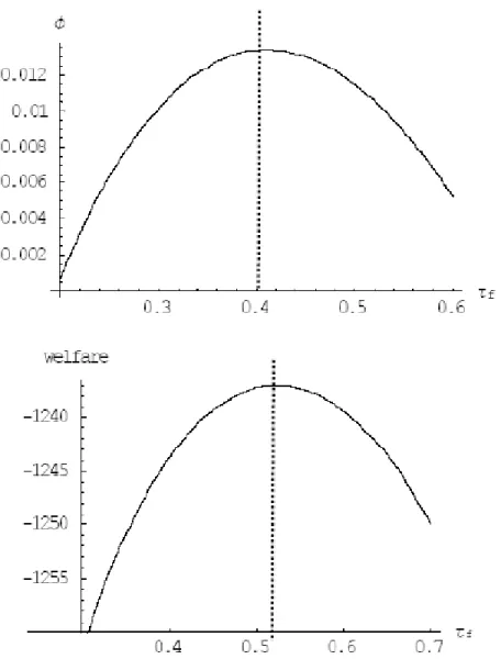
(Insert Figure 4 about here!)

It is simple to see that in equation (36) the agent's welfare is an increasing function of the economic growth rate6, . However7, because c(0), f(0), and s(0) also depend

on f, s, and g, welfare maximization may not be equivalent to growth maximization.

This is shown in Figure 4, where we select the parameters as:  0.5, 0.35,  0.15,

0.05

 ,  0.05,  1.1, g0.5, and s 0.05. We find that the optimal federal

income tax rate, which maximizes growth is around 0.4. However, the optimal federal

income tax rate, which reaches the maximum welfare, is around 0.5. Therefore, growth- and the welfare-maximizing taxes are not equivalent in this case.

5.2 The Growth-maximizing Taxes

We now focus on finding the optimal taxes for growth maximization. In fact, differentiating equation (35) with respect to f, s, and g yields

1 1 ( ) ( ) [ ( ) (1 ) ] 0 1 1 1 s s s f f f s f g g g g g         _{     }                 , (38)        

6_{In fact, differentiating on equation (36) with respect to  yields}

1 1 2 ( ( )) [ ( ) ( )] ( (1 ) ) U                         _  _  _{ }  _      . Therefore, we have U 0     when   .

1 1 1_{( ) ( ) { ( )( )} 1 1 1 1 1 (1 )[ ( )( ) ( ) ]} 1 1 1 1 0, s s s s f f s s s f s f g g g g g g g g g g g g          _{  }                                 (39) and 1 1 1 (1 ) ( ) ( ) [ ( ) ( ) ] 0. 1 1 1 1 1 s s s s f s f f g g g g g g g g          _{      }    _{       }       (40) Thus, we have ( ) (1 ) 1 s f f s g g          , (38’) ( ) (1 )[ ( ) ( )] 1 1 1 s s s f f s s f g g g g g g                 , (39’) and ( ) 1 1 s s f g g g          . (40’)

Equation (40') yields the same expression as equations (38') and (39'). Hence, we know that optimal choices of f, s, and g are interdependent. The choice of the

federal matching grant is endogenous in the following sense: once g is chosen from the interval (0,1), federal income tax and local income tax are determined by (38') and (39'). From equations (38') and (39'), we obtain the optimal tax rates as8

f g

    (41) and

s g

    , (42) for the federal government and local government, respectively.

Once g is given in the interval (0,1), the federal and local income taxes are

determined by their productiveness and the matching rate multiplied by the productivity of local public spending. The aggregate optimal tax rate is just the sum of the

8_{The Jacobian matrix at the optimal taxes can be derived as}

2 2 1 1 1 1 1 1 1 1 1 1 1 (1 ) ( ) ( ) ( ) ( ) g g g g g g                                                 _{  }            .

productiveness of federal and local expenditures:

s f

     . (43) With the choices of tax rates and transfer specified in equations (41) and (42), the growth-maximizing growth rate is

2 1_[   _]             .

We should say something about the effects of optimal government matching transfer and effects of the matching transfer on the growth. In the last section, we showed the government matching transfer can affect growth but the optimal choices of government matching transfer and the tax rates are interdependent. This occurs because, from equations (6) and (7), we have

( _{s f})

f  s   y.

The government transfer becomes an independent variable. We can also derive the equation with only the federal government income tax rate and government matching transfer; thus, the local government income tax rate becomes an independent variable.

The effects of government matching transfer in the last section are based on the selected federal and local income tax rates. Thus, we obtain the effects shown in Figure 3. In addition, given the local income tax rate, from equations (38') and (40') we can determine the optimal choices for the government matching transfer and federal income tax rate.

6. A More General Framework

We can extend our analytical framework to a more general one and consider more tax rates. The same set up is used for the federal government but we introduce two more taxes for the typical local government. It now levies three taxes: a local income tax (such as the case of state income tax in the United States) at the rate of s, a consumption tax

c

 and a property tax (capital tax in our model) _k. The federal government also makes a transfer to the local government in the form of a matching grant for local public spending at the rate of g. If both levels of government maintain balanced budgets, then budget constraints (6) and (7) can be written as

f

and

s k c

s y k c gs , (45) respectively.

Hence, the federal government public spending, f , is equal to its total income tax,

fy

 , minus its transfer to the local government, gs. The local government's spending is financed by its income tax, sy, its property tax, kk, its consumption tax, cc, and the

grant it receives from the federal government, gs.

In a similar way, we derive a highly nonlinear equation for the growth rate :

1 ₁ ( ( , , , , , , , , , , , )) (1 ) k f s k c f s g      _{            }            , (46) where      ( , , , , , , , , , , , )f s k c g      is given by 1 1 1 1 1 1 ( , , , , , , , , , , , , ) 1 {[( ) ]( ) 1 1 1 (1 ) } { ( ) 1 1 1 1 (1 ) 1 ( ) 1 1 1 (1 ) f s k c f s c k f s c f s k c k s k c f s f s k c k c f s g g g g g g g g g g g g                                      _                                                                 1 1 } . c k c g             

Note that  appears on both sides of equation (46). Therefore, the growth rate is implicitly defined as a function of f , s, k, c, g,  , , ,  ,  , and  .

For the endogenous growth rate to be positive, we must impose 0, and from the TVC

(1 ) 0

    ,

which is also the condition for a bounded discounted utility over the infinite horizon. Given such an extended framework with government expenditures and taxes by two levels of government and intergovernmental transfer, we cannot hope that growth-maximizing choices of tax rates and the transfer rate will be consistent with the welfare-maximizing ones. The simple case in Barro's (1990) analysis whereby growth maximization coincides with welfare maximization disappears here. In fact, when both a local consumption tax and a local property tax are present, welfare is a complicated function of the growth rate, which in turn is a complicated function of various taxes and

the federal transfer, as shown in equation (46).

7. Conclusion

This paper has extended the Barro (1990) model with single aggregate government spending and one flat income tax to include public expenditures and taxes by multiple levels of government. We have derived the rate of endogenous growth under quite general specifications of preferences and production technology. With simulations, we have examined how the rate of endogenous growth changes with respect to federal income tax, local income tax, and federal transfer. We have also discussed growth-maximizing choices of income taxes and federal transfer. In addition, we extend our model to a more general framework including a local consumption tax and local property tax. A preliminary simulation analysis has shown that the local property tax has the largest negative impact on the rate of economic growth, whereas a local consumption tax is always growth enhancing. This finding contrasts with that of Rebelo (1991), who shows that a consumption tax has no effect on the growth rate.

The model in this paper sets up a positive framework for evaluating how the assignment of taxes and expenditures among different levels of government and intergovernmental transfers affect economic growth. Our analysis also sheds light on the role of intergovernmental transfers in regional economic growth. If a local government has sufficient revenue base, federal transfers seem to reduce the growth rate. Even if local revenue is not sufficient, the rise in the rate of federal transfer increases the growth rate to a very modest degree. Of course, the model is also useful for normative discussions of the welfare- and growth-maximizing choices of taxes, transfers, and expenditures in the context of fiscal federalism.

In future, we will add two more dimensions: one will be to follow Arrow and Kurz (1970) and introduce public consumption and public capital accumulation at both the federal and local levels into the endogenous growth model; the other will be to formulate a game-theoretical growth model and allow strategic interactions between the federal government and multiple local governments in the choices of taxes, public expenditures, and intergovernmental transfers.

References

Arrow, K., and M. Kurz (1970) Public Investment, the Rate of Return and Optimal Fiscal Policy,Johns Hopkins University Press.

Aschauer, D. (1989) “Is government spending productive?” Journal of Monetary Economics 23, 177-200.

Barro, R.J. (1990) “Government spending in a simple model of endogenous growth” Journal of Political Economy 98, S103-S125.

Bird, R. (1993) “Threading the fiscal labyrinth: Some issues in fiscal decentralization” National Tax Journal 46, 207-227.

Brueckner, J. (1996) “Fiscal federalism and capital accumulation” Mimeo. University of Illinois at Urbana-Champaign.

Davoodi, H. and H. Zou (1998) “Fiscal decentralization and economic growth: A cross-country study” Journal of Urban Economics 43, 244-257.

Devarajan, S, V. Swaroop, and H. Zou (1996) “The composition of government expenditure and economic growth” Journal of Monetary Economics 37, 313-344.

Devarajan, S, D. Xie, and H. Zou (1998) “Should public capital be subsidized or provided?” Journal of Monetary Economics 41,319-331.

Easterly, W. and S. Rebelo (1993) “Fiscal policy and economic growth: An empirical investigation” Journal of Monetary Economics 32, 417-458.

Glomm, G. and B. Ravikumar (1994) “Public investment in infrastructure in a simple growth model” Journal of Economic Dynamics and Control 18, 1173-1187.

Gramlich, E. (1993) “A policy maker's guide to fiscal decentralization” National Tax Journal 46 229-235.

Hulten, C. (1994) “Optimal growth with infrastructure capital: Theory and implications for empirical modeling” Mimeo. University of Maryland.

King, R.G. and S. Rebelo (1990) “Public policy and economic growth: Developing neoclassical implications” Journal of Political Economy 98, S126-S150.

Oates, W. (1972) Fiscal Federalism, New York, Harcourt Brace Jovanovich.

Oates, W. (1993) “Fiscal decentralization and economic development” National Tax Journal 46, 237-243.

Rebelo, S. (1991) “Long-run policy analysis and long-run growth” Journal of Political Economy 99, 500-521.

Rivlin, A. (1992) Reviving the American Dream: The Economy, the States, and the Federal Government, Brookings Institution, Washington, D.C.

Turnovsky, S. (2000) Methods of Macroeconomic Dynamics, MIT Press.

Zhang, T. and H. Zou (1998) “Fiscal decentralization, public spending, and economic growth in China” Journal of Public Economics 67, 221-240.

Zou, H. (1995) “Dynamic effects of federal grants on local spending” Journal of Urban Economics 36, 98-115.

Zou, H. (1996) “Taxes, federal grants, local public spending, and growth” Journal of Urban Economics 39, 303-317.

Figure 1: Growth rate versus federal government income tax rate. The parameters are:  0.5, 0.4, 0.05,  0.05,  2, g0.5, and s 0.1; in the case of

  : 0.35,  0.15;   :  0.25,  0.25;   : 0.15, 0.35.

Figure 2: Growth rate versus local government income tax rate. The parameters are:

0.5

 , 0.4, 0.05,  0.05,  2, g0.5, and  _f 0.2; in the case of   :

0.35

Figure 3: Growth rate versus federal government matching grant for locality g. The parameters are:  0.5,  0.4,  0.05,  0.05,  2, _f 0.2, and _s 0.1; in the case of   :  0.35,  0.15;   : 0.25,  0.25;   :  0.15, 0.35

Figure 4: Growth maximization and welfare maximization. The parameters are:

0.5