and climate variability in vineyard regions
Andrew Sturman
1*, Peyman Zawar-Reza
1, Iman Soltanzadeh
2, Marwan Katurji
1, Valérie Bonnardot
3,
Amber Kaye Parker
4, Michael C. T. Trought
5,
Hervé Qu
é
nol
3, Renan Le Roux
3, Eila Gendig
6and Tobias Schulmann
71Centre for Atmospheric Research, University of Canterbury, Christchurch, New Zealand 2MetService, Wellington, New Zealand
3LETG-Rennes COSTEL, UMR 6554 CNRS, Université Rennes 2, Rennes, France 4Department of Wine, Food and Molecular Biosciences, Lincoln University, Lincoln, New Zealand
5Plant & Food Research Ltd., Marlborough Wine Research Centre, Blenheim, New Zealand 6Department of Conservation, Christchurch, New Zealand
7Catalyst, Christchurch, New Zealand
This article is published in cooperation
with the ClimWine international conference held in Bordeaux 11-13 April 2016. Guest editor: Nathalie Ollat
Grapevines are highly sensitive to environmental conditions, with variability in weather and climate (particularly temperature) having a significant influence on wine quality, quantity and style. Improved knowledge of spatial and temporal variations in climate and their impact on grapevine response allows better decision-making to help maintain a sustainable wine industry in the context of medium to long term climate change. This paper describes recent research into the application of mesoscale weather and climate models that aims to improve our understanding of climate variability at high spatial (1 km and less) and temporal (hourly) resolution within vineyard regions of varying terrain complexity. The Weather Research and Forecasting (WRF) model has been used to simulate the weather and climate in the complex terrain of the Marlborough region of New Zealand. The performance of the WRF model in reproducing the temperature variability across vineyard regions is assessed through comparison with automatic weather stations. Coupling the atmospheric model with bioclimatic indices and phenological models (e.g. Huglin, cool nights, Grapevine Flowering Véraison model) also provides useful insights into grapevine response to spatial variability of climate during the growing season, as well as assessment of spatial variability in the optimal climate conditions for specific grape varieties.
Keywords: WRF model, weather and climate, grapevine response, Marlborough, New Zealand Abstract
Received 10 July 2016; Accepted : 18 October 2016 DOI: 10.20870/oeno-one.2016.0.0.1538
100 -OENO One, 2017, 51, 2, 99-105
©Université de Bordeaux (Bordeaux, France)
A. Sturman et al.
Introduction
It is well known that the temporal and spatial variability
of weather and climate within vineyard regions has an
important influence on grapevine response and therefore
wine production (quality and quantity). To understand
the potential consequences of climate change for
viticulture in regions of complex terrain it is important to
investigate this influence across a range of time and space
scales in order to appropriately manage future risks to the
local wine industry. However, many vineyard regions
have a poor record of meteorological, as well as
phenological, observations. We therefore need to explore
other ways of investigating the variation of weather and
climate across wine-producing regions and its influence
on the grapevine at the vineyard scale. Physics-based
mesoscale atmospheric numerical models are tools that
can be used to provide a good understanding of the
fine-scale variability of weather and climate across a vineyard
area, even in regions of complex terrain (Bonnardot and
Cautenet, 2009; Soltanzadeh
et al.
, 2016). These models
have been used to address a range of other applied
problems, including dust and air pollution dispersion,
wild fire behaviour and wind energy resource assessment
(Purcell and Gilbert, 2015; Alizadeh Choobari
et al.
,
2012; Simpson
et al.
, 2013; Sturman
et al.
, 2011; Titov
et al.
, 2007).
The key research question addressed in this paper is
therefore: what can mesoscale numerical models tell us
about weather/climate variability at vineyard scale and
its influence on grapevine response? This question is
addressed by applying an internationally well-known
mesoscale atmospheric model to New Zealand’s most
important vineyard region.
Research methodology
The main feature of this research is the application of the
Weather Research and Forecasting (WRF – Skamarock
et al.
, 2005) model to simulate local weather/climate in
vineyard regions in complex terrain for both short term
weather forecasting in support of frost protection and
spraying activities, as well as longer term investigation
of the spatial and temporal variability of vineyard scale
climate. In the latter case, the aim is to demonstrate the
usefulness of atmospheric mesoscale models for:
- identifying the major influences on local weather and
climate (sea breezes, foehn effect, cold air drainage and
ponding, etc.) in vineyard regions, essentially identifying
the main contributions to the climate component of the
terroir.
- investigating the influence of local and regional
weather/climate on grapevine response and climate risk
factors for viticulture through the coupling of mesoscale
models with bioclimatic and crop models.
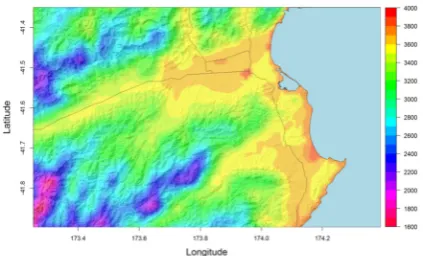
Marlborough region
Marlborough is the most important wine-producing region
of New Zealand, producing more than 70 % of the wine
exported from the country. It is located in the northeastern
part of the South Island in a region of complex terrain,
with significant relief and altitudes reaching more than
1500m in a number of places (Figures1 and 2). The main
vineyard areas are mostly located on the lower-lying flood
T
!""#
$"""#
%"""# &'()*+,-./01-(23/4 2222256718/,9
:;6#-6<2=/>/1/,/< ?/'@-1-2A(8/,9B
C*+>@8/,9
?/'1/>*
22?/'+/+/D/ :=/+>',)*+*6E@B
F/,>-+)6+4
F-,>+/82G>/E*
3/42*H2I8-,>4
?/'D/+/ =/+8)*+*6E@ C-8(*,
T
Figure 2 - Distribution of vineyards within the Marlborough region in 2011, with the locations of weather stations operating between 2013 and 2015.
The filled circles are sites of long-term records, these were supplemented by the red sites for the study period. Vineyard map
provided by the Marlborough District Council.
Figure 1 - The location of vineyard regions in New Zealand (after Sturman and Quénol 2013).
plains of the two main valleys of the Wairau and Awatere
rivers.
Sauvignon blanc is the dominant grape variety planted in
the region, following by Pinot noir, Chardonnay and Pinot
gris (Figure 3).
WRF model setup
The WRF was set up using a four-level nested grid
configuration, as shown in Figure 4a, for computational
efficiency. The model was run twice per day producing
hourly predictions of meteorological parameters such as
air temperature and pressure, wind speed and direction,
and atmospheric humidity at 1 km resolution over the
Marlborough region (Figure 4b).
Initial assessment of the WRF model performance through
comparison with automatic weather station data in
Marlborough suggests that there is a cold bias of between
0.5 and 1.0 °C. Potential cold bias of model predictions
has previously been recognized (Steele
et al.
, 2014; Hu
et al.
, 2010), and needs to be allowed for when interpreting
analysis of spatial patterns across the region. This cold
bias will be the subject of further research so that
appropriate adjustments can be made.
In addition to seasonal maps of key variables (average
daily maximum, minimum and mean temperature), maps
of accumulated degree-days were derived from hourly
temperature predictions two metres above ground level
(Parker
et al.
2011, 2013), as shown in Figure5. Seasonal
maps of using the parameters of the GFV model for a
temperature summation (base temperature of 0 °C, start
date of 29 April) and other bioclimatic indicators were
also produced.
It should be mentioned that the GFV model was not
developed to provide a degree-day accumulation over the
whole growing season, but to set temperature sum
thresholds at which a given grape variety reaches a given
phenological stage (flowering or véraison). Although the
results produced here do not strictly reflect the original
rationale of the GFV model, it is still possible to derive a
temperature summation for the growing season (as shown
in Figure 5), allowing analysis of inter-annual and
intra-regional patterns of heat accumulation.
Results
1. Coupling WRF model output with bioclimatic
indices
By coupling the WRF model output with bioclimatic
indices and phenological models it is possible to provide
a spatial analysis of the suitability of a vineyard region to
a range of different grapevine varieties. As shown in
Figure 6, the key indices/models examined in this paper
are:
- Mean growing season temperature (1 October to 30
April);
- Huglin index (1 October to 31 March);
- Grapevine Flowering Véraison model (29 August to
30 April).
The three maps in Figure6 show significant commonality.
For example, the influence of the complex terrain of the
region is clearly evident in all three maps, with altitude
and distance from sea having an important influence on
the thermal environment of the region. However, some
- 101 - ©Université de Bordeaux (Bordeaux, France)OENO One, 2017, 51, 2, 99-105
Figure 3 - The breakdown of vineyard area in the Marlborough region by grape variety in 2016.
Figure 4 - The WRF nested grid configuration, showing terrain height, a) for all four grid domains (27, 9, 3 and 1 km resolution), and b) the high-resolution domain.
and Pinot gris (Figure 3).
I
Figure 5 - Example map of temperature summation over the Marlborough region from 29 August 2013 to 30 April
2014 calculated according to the GFV model using a threshold of 0 °C
and based on WRF model temperatures.
and Pinot gris (Figure 3).
differences also occur between the maps, with the mean
growing season temperature and the GFV temperature
summation (Figures 6a and c) picking out the warming
effect of the sea along a narrow strip near the coastline,
while the Huglin index (Figure 6b) indicates greater
accumulated heat in the central part of the Wairau Valley.
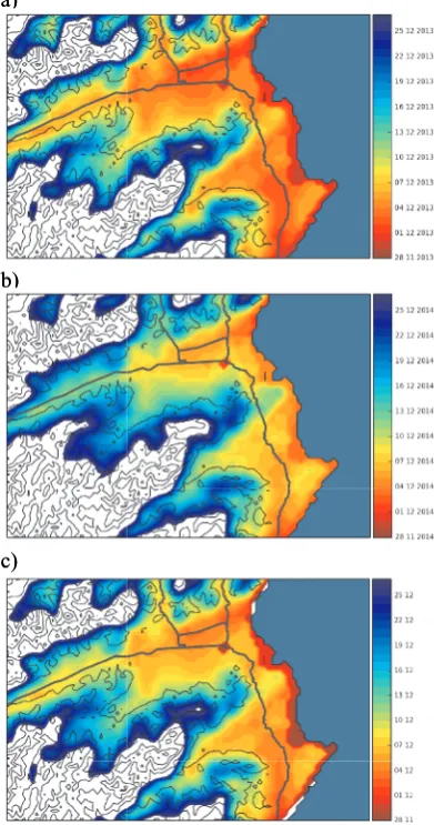
2. Integration of WRF with the GFV model: 50 %
flowering/véraison dates
The GFV model has the following parameters (daily
degree-day accumulations) that can be used for prediction
of flowering and véraison for Sauvignon blanc: F* =1282
(50 % flowering); 2528 (50 % véraison), where F* is the
critical temperature sum (threshold = 0 °C, starting on
the Northern Hemisphere 60th day of the year - 29 August
in the Southern Hemisphere). The WRF model output
can be used with the GFV model to map the timing of
flowering and véraison across vineyard regions, as shown
for Marlborough in Figure 7.
Figures 7a and b illustrate the extent of inter-seasonal
variability in the development of flowering across the
region. Using a combination of WRF model output and
the GFV model, the development of key phenological
phases can be mapped across a region of complex terrain
like Marlborough, to provide the basis for predicting
the magnitude and timing of harvest for different parts of
the region.
3. Optimal mean growing season temperatures for
key Marlborough grape varieties
The WRF-predicted spatial variation in mean growing
season temperature (GST) can also be mapped and
compared with published optimal ranges of values
102 -OENO One, 2017, 51, 2, 99-105
©Université de Bordeaux (Bordeaux, France)
A. Sturman et al.
a)
b)
c)
a)
o
s
a
b)
b)
c)
e
.
e
y
n
n
a
t
g
n
a)
b)
c)
o
s
a
b
a)
b
b)
c
c)
e
.
e
y
n
n
a
t
g
n Figure 6 - Maps of: a) mean growing season
temperature, b) Huglin index, and c) GFV temperature summation, based on the 2008-9 to 2013-14 growing
seasons
in the Marlborough region.
associated with different grape varieties (Jones, 2006 and
2007):
- Pinot gris [13 – 15.2 °C],
- Chardonnay [14.2 – 17.2 °C],
- Pinot noir [14 – 16.2 °C],
- Sauvignon blanc [14.8 – 18 °C].
(approximate values extracted from graphs in Jones, 2006
and 2007)
In Figure8, the different mean growing season temperature
ranges considered optimal for the four most important
Marlborough grape varieties are plotted using the same
colour scale, so that the red colours at either end of the
scale indicate marginal regions, while the blues and greens
represent the most optimal areas for each grape variety.
Based on the WRF-derived temperatures and published
optimal temperature ranges for grape varieties, the most
optimal grape variety for the Marlborough region appears
to be Pinot noir, rather than Sauvignon blanc, which is by
far the dominant variety in the region. There are three
possible reasons for this anomalous result. First, the cold
bias of the WRF model tends to suggest that both
Sauvignon blanc and Chardonnay are less optimal than
they really are, while Pinot noir and Pinot gris appear to
be more optimal.
Second, the ranges of GST used to represent optimal
growing conditions for the different grape varieties are
based on typical values of GST obtained from regions
where those varieties are currently successfully grown
(Jones, 2006 and 2007). This rather assumes that the
present-day thermal environment is the main reason for
the grapes being located where they are, when in fact
historical and cultural factors may also be important.
Third, Marlborough, and in particular the Awatere Valley,
produces a grassy style Sauvignon blanc. The grapes are
harvested at a lower level of ripeness (at a higher
3-isobutyl-2-methoxy-pyrazine content) than in other parts
of the world where Sauvignon blanc is produced, and this
creates a distinctive wine style.
Conclusions
The application of mesoscale weather/climate models to
vineyard regions such as Marlborough (in New Zealand)
provides improved knowledge of the unique features of
the weather/climate (sea breezes, foehn winds,
mountain/valley winds, cold air ponding, etc.) and their
contribution to the local ‘terroir’. Models such as WRF
can also be used to investigate the relationship between
weather/climate and key phases of grapevine development
at vineyard scale within wine-producing regions.
Variability of climate can be investigated across vineyard
regions at high resolution using such models, allowing
- 103 - ©Université de Bordeaux (Bordeaux, France)OENO One, 2017, 51, 2, 99-105
Figure 8 - Maps of optimal mean GST ranges for the main Marlborough grape varieties:
a) Pinot gris, b) Chardonnay, c) Pinot noir and d) Sauvignon blanc, based on WRF model output for 2008-2014.
S
T
!
a)
b)
c)
d)
!
!
!
!
!
!
!
a)
!
!
!
!
!
b)
!
!
!
!
!
!
!
!
!
!
c)
!
!
!
!
!
d)
!
!
!
!
!
!
identification of optimal/marginal areas for winegrape
production and climate risk assessment based on various
bioclimatic indices. Such analysis can also be used to
assess the robustness of vineyard regions to longer term
climate change, including how much change would be
required to make a region unsustainable with respect to
specific grape varieties.
The use of the WRF model to assess the suitability of
specific grape varieties in the Marlborough region suggests
that we need to investigate the origin and nature of the
cold bias in model predictions in order to provide more
accurate simulations of near-surface temperatures and
hence bioclimatic indices. It is also important to improve
understanding of the relationship between climate
parameters such as average growing season temperature
and grapevine response to be able to better assess the
future of quality wine production in specific areas in
response to changing climate. It is therefore important
that future work addresses the limitations identified in
combining WRF modelled temperatures with bioclimatic
indices by coupling WRF with phenophase models at a
higher temporal and spatial resolution.
The suitability of grape varieties to specific areas also
depends on the style of wine. For example, Marlborough
Sauvignon blanc is generally harvested at a commercial
soluble solids (SS) of 20.5 to 21.5 °Brix. Other regions
and styles may require a higher SS and therefore take
longer to achieve that target. It may therefore be more
logical to base suitability of grape varieties on the
temperature summation it takes to reach a particular SS
target (based on the GFV model).
The effects of manipulation of the grapevine environment
at vineyard scale should also be integrated into more
comprehensive modelling systems, as the effects of
variations in the regional climate could be offset by
vineyard management techniques (Webb
et al.
, 2012).
In conclusion, it should be noted that Global Climate
Models (GCMs) provide only a general idea of the
larger-scale changes in climate likely to occur in vineyard regions
over future decades (as discussed by Hannah
et al.
, 2012
and 2013, and van Leeuwen
et al.
, 2013). It is evident
that downscaling GCM output to the regional and local
scales is fraught with difficulty in regions of complex
terrain as the interaction of hemispheric and synoptic
scale processes with local and regional topography can
introduce significant spatial variation in response to large
scale forcing (Sturman and Quénol, 2013). It is therefore
important that methods of dynamical and statistical
downscaling be improved to allow more realistic
assessment of the impacts of climate change on vineyard
regions, in order to develop appropriate and effective
adaptation strategies.
Acknowledgements: The research team are grateful for the funding provided for this research by the Ministry for Primary Industries (New Zealand), and ongoing support of the Department of Geography at the University of Canterbury, Plant & Food Research and the Marlborough Wine Research Centre, Lincoln University, and the COSTEL Laboratory at the University of Rennes 2 (France). James Sturman’s assistance with the final graphics is also much appreciated. We would also like to thank the organisers of the ClimWine2016 Symposium for the opportunity to present our work.
References
Alizadeh Choobari, O., Zawar-Reza, P. and Sturman, A. 2012. Atmospheric forcing of the three-dimensional distribution of dust particles over Australia: A case study.Journal of Geophysical Research – Atmospheres, 117, D11206, 19 pp., doi: 10.1029/2012JD017748
Bonnardot, V. and Cautenet, S. 2009. Mesoscale atmospheric modelling using a high horizontal grid resolution over a complex coastal terrain and a wine region of South Africa. Journal of Applied Meteorology and Climatology, 48, 330-348.
Hannah, L., Roehrdanz, P.R., Ikegami, M., Shepard, A.V., Shaw, M.R., Tabor, G., Zhi, L., Marquet, P.A. and Hijmans, R.J. 2013. Climate change, wine, and conservation. Proceedings of the National Academy of Sciences, 110, 6907-6912.
Hu, X.M., Nielsen-Gammon, J.W. and Zhang, F. 2010. Evaluation of three planetary boundary layer schemes in the WRF model. Journal of Applied Meteorology and Climatology, 49, 1831–1844.
Jones, G.V. 2006. Climate and Terroir: Impacts of Climate Variability and Change on Wine. In: Fine Wine and Terroir – The Geoscience Perspective. Macqueen, R.W., Meinert, L.D. (eds) Geoscience Canada Reprint Series Number 9; Geological Association of Canada; St. John’s, Newfoundland, 247pp.
Jones, G.V. 2007. Climate Change and the Global Wine Industry.Australian Wine Industry Technical Conference, Adelaide, Australia. July 28-August 2, 2007, 8pp. Parker, A.K., García de Cortázar-Atauri, I., Chuine, I.,
Barbeau, G., Bois, B., Boursiquot, J-M., Cahurel, J-Y., Claverie, M., Dufourcq, T., Gény, L., Guimberteau, G., Hofmann, R.W., Jacquet, O., Lacombe,T., Monamy,C., Ojeda,H., Panigai, L., Payan, J-C., Rodriquez Lovelle,B., Rouchaud, E., Schneider, C., Spring, J-L., Storchi, P., Tomasi, D., Trambouze, W., Trought, M., and van Leeuwen, C. 2013. Classification of varieties for their timing of flowering and veraison using a modelling approach. A case study for the grapevine speciesVitis vinifera L. Agricultural and Forest Meteorology, 180, 249-264.
Parker, A. K., García de Cortázar-Atauri, I., van Leeuwen, C., and Chuine, I. 2011. General phenological model to characterise the timing of flowering and veraison ofVitis viniferaL. Australian Journal of Grape and Wine Research, 17, 206-216.
104 -OENO One, 2017, 51, 2, 99-105
©Université de Bordeaux (Bordeaux, France)
energy-wind-mapping-maldives-mesoscale-wind-modeling-report-1-interim-wind-atlas-maldives Simpson, C.C., Pearce, H.G., Sturman, A.P. and Zawar-Reza,
P. 2013. Verification of WRF modelled fire weather in the 2009/10 New Zealand wildland fire season. International Journal of Wildland Fire, 23, 34-45. http://dx.doi.org/10.1071/WF12152.
Skamarock, W.C., Klemp, J.-B., Dudhia,J., Gill, D.O., Barker, D.M., Wang, W. and Powers, J.-G. 2005. A description of the Advanced Research WRF Version 2. NCAR Tech Notes-468+STR.
Soltanzadeh, I., Bonnardot,V., Sturman, A.Quénol,H., Zawar-Reza, P.2016. Assessment of the ARW-WRF model over complex terrain: the case of the Stellenbosch Wine of Origin district of South Africa. Theoretical and Applied Climatology, DOI 10.1007/s00704-016-1857-z Steele, C.J., Dorling, S., von-Glasow, R. and Bacon, J. 2014.
Modelling sea-breeze climatologies and interactions on coasts in the southern North Sea: implications for offshore wind energy. Quarterly Journal of the Royal Meteorological Society, 141, 1821–1835.
Environment, 409, 810-821.
Sturman, A., and Quénol, H. 2013. Changes in atmospheric circulation and temperature trends in major vineyard regions of New Zealand. International Journal of Climatology33, 2609-2621, DOI: 10.1002/joc.3608. Titov, M., Sturman, A.P. and Zawar-Reza, P.2007. Application
of MM5 and CAMx4 to local scale dispersion of particulate matter for the city of Christchurch, New Zealand. Atmospheric Environment, 41, 327-338. van Leeuwen, C., Schultz, H.R., Garcia de Cortazar-Atauri, I.,
Duchêne, E., Ollat, N., Pieri, P., Bois, B., Goutouly, J. P., Quénol, H., Touzard, J.-M., Malheiro, A.C., Bavarescok, L. and Delrot, S. 2013. Why climate change will not dramatically decrease viticultural suitability in main wine-producing areas by 2050. Proceedings of the National Academy of Sciences, 110, E3051-2.
Webb, L.B., Whetton, P.H., Bhend, J., Darbyshire, R., Briggs, P.R. and Barlow, E.W.R. 2012. Earlier wine-grape ripening driven by climatic warming and drying and management practices. Nature Climate Change, 2, 259-264.