Potential of manuka and kanuka for the mitigation of nitrous oxide emissions from NZ dairy farms

(1)

Lincoln

University

Digital

Dissertation

Copyright

Statement

The

digital

copy

of

this

dissertation

is

protected

by

the

Copyright

Act

1994

(New

Zealand).

This

dissertation

may

be

consulted

by

you,

provided

you

comply

with

the

provisions

of

the

Act

and

the

following

conditions

of

use:



_you

_will

_use

_the

_copy

_only

_for

_the

_purposes

_of

_research

_or

_private

_study



you

will

recognise

the

author's

right

to

be

identified

as

the

author

of

the

dissertation

and

due

acknowledgement

will

be

made

to

the

author

where

appropriate



you

will

obtain

the

author's

permission

before

publishing

any

material

from

the

dissertation.

(2)

Potential of manuka and kanuka for the mitigation of nitrous oxide

emissions from NZ dairy farms

A dissertation

submitted in partial fulfilment

of the requirements for the Degree of

Bachelor of Science with Honours

at

Lincoln University

by

Roshean Fitzgerald

Lincoln University

2012

Supervisors:

(3)

Abstract of a dissertation submitted in partial fulfilment of the

requirements for the Degree of Bachelor of Science with Honours.

Abstract

Potential of manuka and kanuka for the mitigation of nitrous oxide emissions

from NZ dairy farms

by

Roshean Fitzgerald

Nitrous oxide (N2O) is a greenhouse gas with a global warming potential 298 times that of carbon

dioxide. Since pre-industrial times, atmospheric levels of N2O have increased from 270 to 319 ppb.

More than a third of emissions are anthropogenic, most of which are due to agriculture. This loss of nitrogen as N2O represents an important economic loss to the agricultural industry. N2O is primarily

produced in soils via the processes of nitrification and denitrification, both of which are biologically driven processes. It is possible that these processes may be perturbed by plants, such as the New Zealand natives: Leptospermum scoparium (manuka) and Kunzea ericoides (kanuka) that are known to contain antimicrobial compounds. Potentially, the strategic planting of manuka or kanuka on NZ dairy farms may reduce N2O emissions. This study aimed to test whether manuka and kanuka

affected soil microbes and specifically altered the production of N2O.

A greenhouse pot trial was conducted using Lolium perenne (perennial ryegrass pasture), manuka and kanuka plants to test whether the latter two reduced the N2O fluxes from the soil when ~200 kg

N ha-1_{dairy shed effluent was added as a nitrogen source. A closed-chamber method was developed}

using 20 L plastic buckets to enable collection of gas samples from the whole pot system. N2O

concentrations were determined using gas chromatography fitted with an electron capture detector. A preliminary trial indicated that manuka plants may reduce N2O fluxes from soil. However, a

full-scale trial did not produce measurable N2O fluxes. This was attributed to the high volume to soil

surface area (0.17 m3_{:0.02 m}2_{) of the chambers used, meaning they provided insufficient sensitivity}

to determine the low N2O fluxes.

Following the unsuccessful greenhouse study, a field trial was carried out using an already established method of field N2O collection. Again a closed-chamber method was used, but, these

chambers had a much lower volume to soil surface area ratio (0.26 m3_{:0.18 m}2_{). N}

(4)

soil beneath 5 year-old kanuka trees were compared with bare ground soil (control) treated with either water or dairy shed effluent. Soil samples were taken from adjacent plots which received the same treatments. For effluent-treated plots, N2O fluxes were higher from the control compared with

kanuka plots; cumulative fluxes were 65 and 13 mg N2O-N m-2, respectively. Soil nitrate levels were

higher under kanuka than control plots, mean values were 17.1 and 3.3 µg g-1_{soil, respectively.}

These findings may indicate an inhibition of denitrification beneath kanuka.

A further experiment demonstrated that 7 days after inoculation, soil Escherichia coli levels in manuka and kanuka pots (average 8 000 cfu g-1_{) were reduced compared with pasture control pots}

(65 000 cfu g-1_).

These experiments demonstrate that manuka and kanuka affect the functioning and survival of soil microorganisms and reduce N2O emissions under some conditions. Further research should focus on

elucidating the mechanisms responsible for this inhibition, and test the range of environmental conditions where these plants may be used effectively.

Keywords:Leptospermum scoparium, Kunzea ericoides, Lolium perenne, N2O, antimicrobial, nitrogen

(5)

Acknowledgements

Firstly I would like to acknowledge my supervisor Brett Robinson who has been very supportive throughout the study, for meeting with me on a regular basis to discuss results and progress, and for being so enthusiastic about the study. To my other supervisors: Timothy Clough, and Nicholas Dickinson thank you for all your help, guidance and advice along the way.

A huge thank you to Hannah Franklin for your help with sample collection and set up of both the nitrous oxide trials, I truely valued your advice and your friendly company, particularly out in the field. I appreciate your interest and enthusiasm for the study and thank you for always being there to bounce ideas off and have discussions.

I would like to thank the technicians who provided friendly and useful advice, and for analysis of samples: Manjula Premaratne, Qian Liang, Lynne Clucas, Leanne Hassall. Thank you Neil Smith for your technical expertise in setting up and providing me with a data logger as well as your help with the development of the nitrous oxide collection chambers for pot experiments. For their useful ideas which helped develop the collection chambers for the pot experiment, thank you Carole Barlow, and Stephen Moore . Rob Sherlock thank you for your ideas and guidance, they were much appreciated. I would like to thank the greenhouse staff Brent Richards and Leona Meachen for their help and for accomodating this experiment.

Thank you to the team at the Centre for Soil and Environmental Research (CSER), particularly Roger Atkinson, and Trevor Hendry for lending us equipment for the field trial, your friendly advice and for being so accomodating.

Thank you Jennifer Prosser, and Jacqui Horswell from Environmental Science and Research (ESR) for supplying advice, help and equipment for the antimicrobial experiment.

I would like to thank the New Zealand Agricultural Greenhouse Gas Research Centre (NZAGRC) and DairyNZ for providing scholarships for my tuition fees and living costs.

(6)

List of Tables

Table 1.1 Summary of potential effects manuka and/or kanuka planted on dairy farms may have on the cycling of nitrogen. ... 4 Table 2.1 Relative (%) comparison of essential oils from manuka (Leptospermum scoparium) and

kanuka (Kunzea ericoides). From Maddocks-Jennings et al. (2005). ... 18 Table 2.2 GC-MS identification of % peak area contributions of components of commercial

essential oils of manuka (Leptospermum scoparium) and kanuka (Kunzea ericoides). From Porter and Wilkins (1998). ... 18 Table 3.1 Soil chemical properties for the Templeton silt loam. Values in brackets represent the

standard error of the mean (n = 3). From Knowles et al. (2011)... 25 Table 3.2 Initial and final manuka and kanuka dry weight yields (g) ± standard error of the mean. .... 36 Table 4.1 Statistical analysis output of significant N2O flux data showing degrees of freedom (d.f.)

for the number of levels (k) and error d.f., and the variance ratio (F), and P-values

(10)

List of Figures

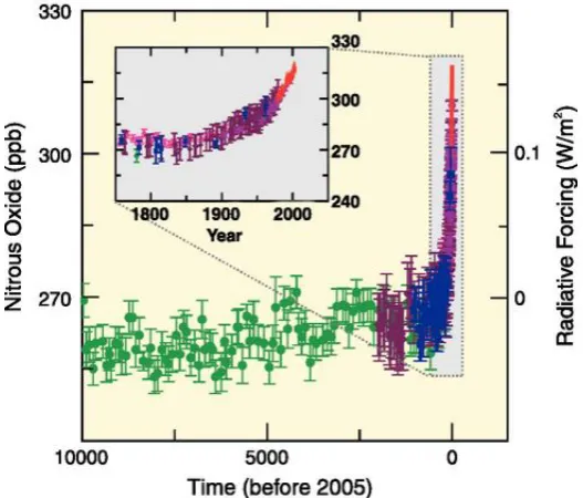
Figure 1.1 Atmospheric concentrations of N2O over the last 10 000 years and since 1750 (inset)

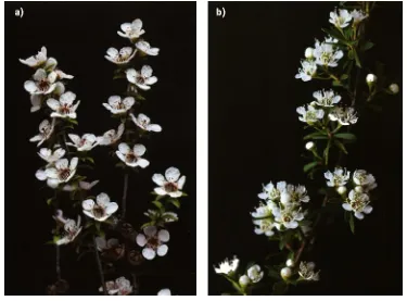
from ice cores and corresponding radiative forcings. From IPCC (2007a). ... 1 Figure 1.2 a) Manuka flowers, leaves and large fruit capsules. b) Kanuka foliage and flowers. From

Wardle (2011). ... 3 Figure 1.3 a) Structural formula of Nitrapyrin. b) Structural formula of α-pinene. ... 4 Figure 1.4 The nitrogen cycle in agricultural systems showing sources of nitrogen loss (blue and

red) and potential sites of inhibition by manuka and kanuka (green). Adapted from McLaren & Cameron (1996). ... 6 Figure 2.1 Schematic diagram of factors affecting: (i) the rate of nitrification and denitrification;

(ii) the N2/N2O ratio of denitrification; and (iii) N2O diffusion from soil (√, affected by

this factor; –, not affected by this factor; ?, unclear if affected by this factor). Shaded boxes represent biological processes. From de Klein et al. (2008). ... 8 Figure 2.2 Chemical structure of leptospermone

(3,5-hydroxy-4-(2-methyl-1-oxopentyl)-2,2,6,6,-tetramethyl-4-cyclohexane-1,3-dione) (Maddocks-Jennings et al., 2005)... 17 Figure 2.3 Nitrous oxide emissions and potential inhibition by the planting of manuka and kanuka,

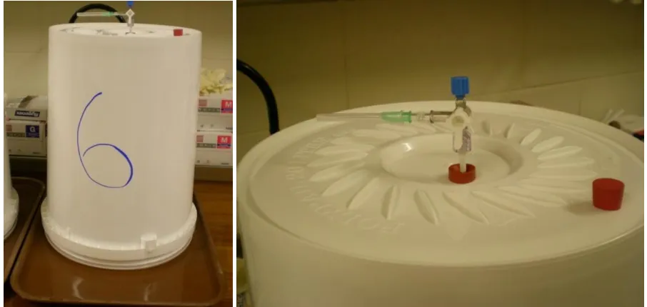
compared with pasture. ... 19 Figure 3.1 Gas collection chamber setup for nitrous oxide measurements (left). Gas collection

valve and needles in top of chamber (right)... 21 Figure 3.2 The hardware associated with the SRI 8610 Gas Chromatograph. ... 22 Figure 3.3 Method testing measurements taken 15 and 30 minutes following the injection of 2 µL

L-1 _{of N}

2O standard into the collection chamber. Error bars are standard error of the

mean (n = 3). ... 22 Figure 3.4 Method testing measurements taken at 15, 30, 60, 120, 180, 240 and 300 minutes

following the injection of 1 µL L-1 _{of N}

2O standard into the collection chamber. Error

bars are standard error of the mean (n = 6). ... 23 Figure 3.5 Method testing measurements taken at 15, 30, and 60 minutes following the injection

of 0.5 µL L-1 _{of N}

2O standard into the collection chamber compared to a blank

(ambient air). Error bars are standard error of the mean (n = 3). ... 24 Figure 3.6 Pots in the greenhouse on 19 December 2011 (left), and 31 January 2012 (right). ... 25 Figure 3.7 Effluent application to pots, 26-30 April 2012. ... 26 Figure 3.8 Experimental setup, showing plants in greenhouse ready to be sampled (left) and

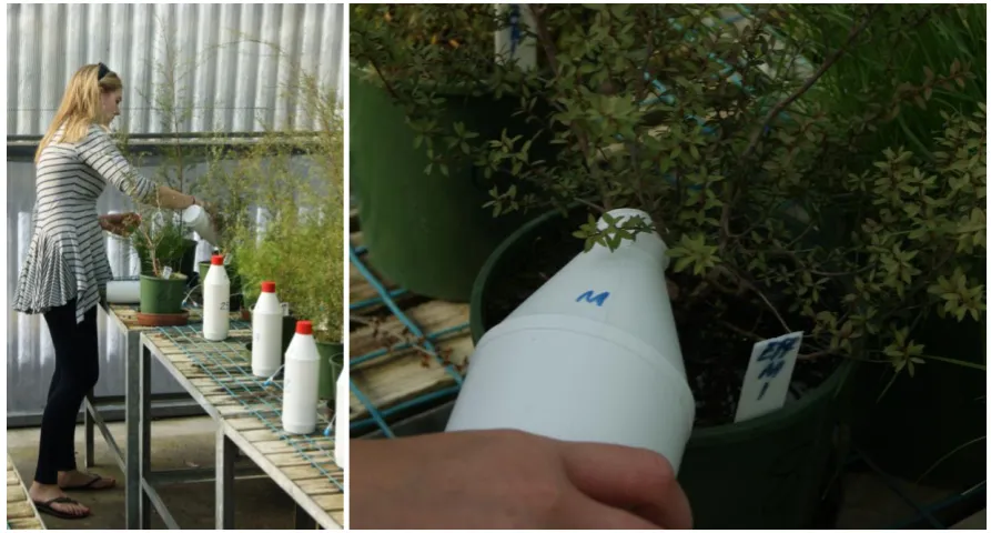
sample chambers in position during gas sampling (right). ... 27 Figure 3.9 HydrosenseTM_{moisture probe used to determine soil moisture content (left). Data}

logger setup for temperature probes (right). ... 29 Figure 3.10 Preliminary nitrous oxide fluxes (µg N2O-N m-2 h-1) beneath plant species: pasture (P),

manuka (M), kanuka (K) following application of ~200 kg N ha-1_{dairy shed effluent.}

Error bars are standard error of the mean (n = 3). ... 31 Figure 3.11 Preliminary N2O concentrations (µL L-1) for blank (B), pasture (P), manuka (M), and

kanuka (K) species following application of ~200 kg N ha-1_{dairy shed effluent. Error}

bars are standard error of the mean (n = 3). ... 31 Figure 3.12 Examples of the results obtained from the nitrous oxide (N2O) concentrations (µL L-1)

(11)

Figure 3.13 Percentage (%) distribution of R2_{values obtained by linear regression of N} 2O

concentrations against time sample taken. ... 32

Figure 3.14 Relationship between nitrate (NO3-) concentration (mg NO3--N L-1 soil) extracted in soil water and time since treatment application, for pasture (P), manuka (M), and kanuka (K) species treated with effluent. Error bars are standard error of the mean. ... 33

Figure 3.15 Soil pH under the control and effluent treatments and species pasture (P), manuka (M) and kanuka (K). Error bars are standard error of the mean (n = 3). See section 3.3.8 for a description of how average pH and standard errors were calculated. ... 34

Figure 3.16 Estimated moisture content (%) in pots at 1, 7 and 14 days after treatment application for pasture (P), manuka (M) and kanuka (K) species treated with a) control and b) effluent. Error bars are standard error of the mean (n = 5). ... 35

Figure 4.1 a) Map showing field site location, Lincoln University Dairy Farm. b) Map of the field site showing plots: control (bare soil) plots (), and kanuka plots (). ... 40

Figure 4.2 Native plantation field site (Lincoln University Dairy Farm) at various stages of its development. ... 41

Figure 4.3 Bare soil sites with (left) and without (right) gas collection chambers. ... 42

Figure 4.4 Kanuka sites with (left) and without (right) gas collection chambers... 42

Figure 4.5 Field gas collection chamber setup. ... 43

Figure 4.6 Collection of gas samples. ... 44

Figure 4.7 Gas sampling syringe and needle setup. ... 44

Figure 4.8 Nitrous oxide (N2O) fluxes (µg N2O-N m-2 h-1) for control (bare soil) (C) plots and kanuka (K) plots treated with either water (W) or effluent (E). Error bars are standard error of the mean (n = 5). ... 46

Figure 4.9 Soil pH of field moist soil with time for control (bare soil) (C) plots and kanuka (K) plots treated with either water (W) or effluent (E). Error bars are standard error of the mean (n = 5). See section 3.3.8 for a description of how average pH and standard errors were calculated. ... 47

Figure 4.10 Soil gravimetric moisture content (%) of field moist soil with time for control (bare soil) (C) plots and kanuka (K) plots treated with either water (W) or effluent (E). Error bars are standard error of the mean (n = 5). ... 48

Figure 4.11 Soil nitrate-N per gram of soil with time for control (bare soil) plots (C) and kanuka (K) plots, applied with either water (W) or effluent (E). Error bars are standard error of the mean (n = 5). ... 48

Figure 4.12 Soil ammonium-N per gram of soil with time for control (bare soil) plots (C) and kanuka (K) plots, applied with either water (W) or effluent (E). Error bars are standard error of the mean (n = 5). ... 49

Figure 5.1 Experimental setup of pots in the greenhouse on 17 January 2012. ... 53

Figure 5.2 UV light used to score EC + MUG vials negative (far left) or positive (four to the right) for E. coli. ... 54

Figure 5.3 Survival of E. coli under three contrasting plant species: pasture (P), manuka (M), and kanuka (K) as measured 1, 3 and 7 days after application of E. coli to the surface of the soil. Error bars are standard error of the mean (n = 3). ... 55

(12)

Figure 5.5 Soil moisture content (%) of soil from beneath pasture (P), manuka (M), and kanuka (K) plant species. Error bars are standard error of the mean (n = 3). ... 57 Figure 6.1 Schematic showing potential planting locations of manuka or kanuka on a New Zealand

(13)

Chapter 1 Introduction

1.1 Nitrous oxide (N

2

O)

Nitrous oxide (N2O) is a GHG which has a global warming potential 298 times that of carbon dioxide

(van Zwieten et al., 2009). Since pre-industrial times, N2O levels in the atmosphere have risen from

270 to 319 ppb (Figure 1.1) (IPCC, 2007a). More than a third of all N2O emissions are anthropogenic

and are primarily due to agriculture (IPCC, 2007a). In New Zealand, there has been a 25.5% increase in N2O emissions from agricultural soils since 1990, caused by nitrogen fertiliser use and an increase

in animal excreta (Ministry for the Environment, 2012). The loss of nitrogen in the form of N2O

represents an important economic loss to producers and consumers of agricultural products (van Zwieten et al., 2009).

Figure 1.1 Atmospheric concentrations of N2O over the last 10 000 years and since 1750 (inset)

from ice cores and corresponding radiative forcings. From IPCC (2007a).

N2O is produced in the soil by several processes that may occur simultaneously within different

microsites of the same soil (Baggs, 2008). Most N2O evolved from soils is produced by biological

(14)

Nitrification involves the oxidation of ammonia (NH3) to nitrate (NO3-) which is carried out by

autotrophic bacteria and archaea in aerobic conditions (DeLuca et al., 2009). These include: ammonia-oxidising bacteria, autotrophic nitrite oxidising bacteria, ammonia oxidising archaea-bacteria, and heterotrophic nitrifying bacteria and fungi (de Klein et al., 2008). However in low oxygen concentrations nitric oxide (NO) and N2O can be formed as by-products of NH4+ oxidation

(Kim & Hollocher, 1983).

Denitrification is the process by which NO3- or nitrite (NO2-) is reduced to dinitrogen gas (N2), of

which both NO and N2O are obligate intermediates. This occurs in the absence of oxygen and is

carried out by heterotrophic facultative anaerobes (which can use both O2 and NO2- or NO3- as

electron acceptor). The four enzymes involved are: nitrate reductase, nitrite reductase, nitric oxide reductase and nitrous oxide reductase (van Zwieten et al., 2009; Uchida, 2010). Figure 1.4 illustrates soil processes resulting in losses of nitrogen (N) from agricultural systems. The loss pathways with negative environmental consequences are NO3- leaching and gaseous losses of N2O.

1.2 Inhibition of the nitrogen cycle by plants

For many years it has been hypothesized that plants release compounds from their root systems that are capable of inhibiting the nitrification process. A bioassay experiment with exudates from a tropical pasture grass Brachiaria humidicola showed a strong inhibitory effect on Nitrosomonas

europaea (a nitrifying bacteria) function and were shown to inhibit nitrification in air-dried and then

rewetted soil. Results showed that the release of biological nitrification inhibition (BNI) compounds had no negative effect on soil microbial populations or plant growth promoting microorganisms, though effectiveness of BNI varied with soil type (Gopalakrishnan et al., 2009). Sorghum (Sorghum

bicolor) has been shown to have significant BNI capacity, the active constituent was identified as

methyl 3-(4-hydroxyphenyl) propionate. BNI compound release from roots is a physiologically active process, stimulated by the presence of ammonium. This may be a useful tool for decreasing the emission of nitrogenous greenhouse gases such as N2O from soil and reducing off-farm impacts

associated with NO3- leaching (Zakir et al., 2008).

1.2.1 Manuka and kanuka

(15)

easily dispersed by wind. Manuka is the most abundant New Zealand shrub, and often forms closed stands up to 8 m tall. Kanuka often co-dominates with manuka in seral shrubland but can grow to 20 m tall (Wardle, 2002).

Figure 1.2 a) Manuka flowers, leaves and large fruit capsules. b) Kanuka foliage and flowers. From Wardle (2011).

Inhibition of the nitrogen cycle by manuka and kanuka

Currently there are no studies on nitrification inhibition caused by manuka or kanuka plants. However, inhibition by monoterpenes with a similar molecular structure to the known nitrification inhibitor: nitrapyrin was suggested as a factor in the extremely low nitrification rates observed in coastal redwood forests. One of these: α-pinene, has been found in manuka and kanuka essential oils (Table 2.2). α-pinene significantly inhibited the growth of Nitrosomonas europaea in batch culture experiments (Ward et al., 1997). This nitrification inhibition demonstrated by one of the constituents of manuka and kanuka essential oils provides promising evidence to support the hypothesis that these plants may be natural nitrification inhibitors. The molecular structures of both nitrapyrin and α-pinene are shown in Figure 1.3. Clough et al. (2010) detected α-pinene in Pinus radiata biochar used in their experiments. This indicated that this compound remained after the biochar manufacturing process of pyrolysis. Thus biochar produced from manuka and kanuka could be mixed into agricultural soils on a larger scale to further reduce the effects of NO3- leaching and N2O

(16)

(17)

Water extracts of manuka, were found to significantly reduce the growth of five pathogenic bacterial strains potentially found in biosolids (Prosser, 2011). These were Salmonella typhimurium, Listeria

monocytogenes, Escherichia coli, Campylobacter jejuni and Clostridium perfringins. However, when

soil was taken from underneath a long-standing manuka forest, effects of the antimicrobial ability on the bacteria from biosolids were not observed. In an attempt to explain this the author suggested that the components that gave rise to the antimicrobial activity in manuka were quickly degraded in the soil; or that manuka plants released antimicrobial agents from roots continuously, which did not remain stable in the soil (Prosser, 2011).

In soils, much of the N cycle is biologically driven by soil bacteria. If the antimicrobial properties of manuka and kanuka are demonstrated in the field, then it is possible that these could have an inhibiting affect on the N cycle in the soil. Figure 1.4 illustrates the many potential sites at which manuka and kanuka could interfere with the N cycle due to inhibition or antimicrobial activity. For example, inhibition of nitrifying bacteria such as Nitrosomonas, Nitrosospira, or Nitrobacter would reduce the amount of nitrogen present as NO3- in the soil and thus reduce its potential to be leached

but is also likely to reduce N2O emissions by reducing the substrate of denitrification. The inhibition

of mineralisation of organic N compounds to NH4+, which can be taken up by plants, would reduce

the negative environmental effects of N, but at the same time less N would be available for plant uptake. Inhibition of denitrifying bacteria would likely reduce the amount of N2O emitted though

(18)

(19)

Chapter 2 Background

Part A

2.1 Greenhouse gases (GHGs)

Greenhouse gases (GHGs) are atmospheric gases that absorb and re-emit long-wave radiation back to the earth’s surface (Pinares-Patino et al., 2009). These are critically important for the regulation of the earth’s surface temperature, as without them, the average temperature would be -19 o_{C instead}

of the current 14 o_{C (IPCC, 2007b)}_{. ‘Warming of the climate system is unequivocal, as is now evident}

from observations of increases in global average air and ocean temperatures, widespread melting of snow and ice, and rising global average sea levels’ (IPCC, 2007a). The IPCC states that ‘most of the observed increase in global average temperatures since the mid-20th_{century is very likely due to the}

observed increase in anthropogenic GHG concentrations’. They go further to state that in fact, it is likely that increases in GHG concentrations alone would have caused more warming than what is currently observed because some warming has been offset by volcanic and anthropogenic aerosols (IPCC, 2007a). New Zealand is the only developed country where agricultural GHG emissions play a major role in its national emission profile (contributing 47.1% (Ministry for the Environment, 2012)). New Zealand has signed up for the Kyoto Protocol and has to take responsibility for its greenhouse gas emissions above 1990 levels. Thus in order to reduce future total GHG emissions there is a need to find ways to mitigate agricultural emissions.

2.2 Factors affecting N

2

O fluxes

The regulation of N2O emissions is very complex, and involves both proximal and distal factors.

Proximal factors include: the rate of nitrification and denitrification, the ratio of the end products of denitrification and the diffusion of N2O through the soil profile (de Klein et al., 2008). These are

affected by distal factors which include those of soil aeration and moisture status, and factors which affect denitrification such as mineral N (particularly NO3-), carbon availability, soil pH and

temperature (Figure 2.1).

Soil aeration affects both the processes of nitrification and denitrification as well as the diffusion of N2O through soil. It is a function of rainfall or irrigation, soil compaction and grazing management (de

(20)

(21)

soluble carbon content of soils and denitrification rate has been shown (Sherlock, 1992). The surface layers of permanent pastures are rich in organic matter with potential for denitrification when fertilised or when urine and dung are deposited. Oxygen depletion can also result from high carbon (C) substrate and thus enhance denitrification. It has been suggested that decomposition of plant litter, animal faeces, and root exudates from the perennial plant cover maintain moderate to high levels of available C in grazed pasture soils for denitrification. The accessibility of C supply to bacteria regulates denitrification. Organic C decreases with depth, and often limits denitrification in subsoils. Limited supply of C is likely to cause partial denitrification resulting in the release of NO and N2O

intermediate gases. As C availability increases the N2O:N2 ratio decreases (Bolan et al., 2004).

Increased N2O fluxes have been observed under peat soils compared with mineral soils and with the

application of sewage sludge materials, containing high levels of water soluble carbon, to land (Sherlock, 1992).

Soil pH affects both the rate of nitrification and denitrification as well as the ratio of N2O:N2

produced by denitrification. Although the range for denitrification of is broad, neutral pH conditions (pH 6-8) are optimal for most denitrifying bacteria (Bolan et al., 2004). In contrast to this, a study by Simek et al. (2002) found no simple relationship between denitrifying enzyme activity (DEA) and soil pH as high DEA was found both in acid and alkaline soils. They also found that the populations of soil denitfiers were adapted to their natural soil pH. In acidic conditions denitrification tends to slow down, but can still occur at pH values as low as 3.5. The mechanism for pH affect on denitrification is unclear. The proportion of N2O increases as pH decreases and N2O is often the dominant product of

denitrification in acid soils. This has been suggested to be due to the presence of increasing amounts of NO2- at lower pH levels (Bolan et al., 2004). A study by Clough et al. (2003) investigated whether

liming could mitigate N2O fluxes from soils amended with urine. It was found that the main effect of

lime was to promote nitrification, which markedly affected N2O fluxes with pH 6.1 (with 500 kg N ha-1

synthetic urine) producing more N2O than any other pH. No optimum soil pH was found for the

higher N treatment of 1000 kg N ha-1_{and denitrification was not found to be enhanced. Sherlock}

(1992) described the optimal pH for nitrification and denitrification to be between 7.0 and 8.0. It was stated that while most of New Zealand’s soils used for pastoral grazing have a pH less than optimal for denitrification, under these more acidic conditions it may be N2O rather than N2 which is the

(22)

Soil temperature affects denitrification through its effect on microbial activity which in general, increases with increasing temperature up to 30 o_{C (Sherlock, 1992; Bolan}_{et al.}_{, 2004). However,}

denitrification can occur at a wide range of soil temperatures between 0 and 75 o_{C. Indirect effects of}

temperature on denitrification include that of O2 solubility and diffusion in water effects.

Temperature is thought to cause temporal fluctuations in denitrification. The optimum temperature for denitrification could differ in different regions. Soil temperature can limit denitrification during winter. In New Zealand, a relatively high denitrification rate is often observed during winter where the soil temperature is below 10 o_{C, this is associated with high soil moisture contents. The N}

2O:N2

ratio produced by denitrification has been shown to decrease with soil temperature (Bolan et al., 2004) particularly below 15 o_{C (Sherlock, 1992). Thus the maximum N}

2O fluxes may not coincide

seasonally with maximum denitrification rates if denitrification goes to completion. Under field conditions, N2O release rates show a diurnal pattern which closely follows the fluctuations in soil

temperature (Sherlock, 1992).

2.2.1 Sources of N

2

O

Animal waste

Grazing ruminants utilize relatively little of the N in feed and 75-90% of their dietary N is recycled back into the system via urine and dung. The proportion of N excreted in urine increases as the N content of the diet increases (de Klein et al., 2008). Ruminant urine is considered to be a major source of N2O emissions in grazed pastoral soils, of which the main N component is urea (CO(NH2)2),

this is rapidly hydrolysed to ammonium (NH4+) (Uchida, 2010). The emission factor (N2O emitted as

percentage of N voided) is generally greater for urine than for dung, with median values of 1.5% and 0.2% for cattle urine and dung respectively (de Klein et al., 2008).

Effluent

Dairy farm effluent (DFE) comprises of animal faeces, urine, and wash-down water collected at the milking shed. This is collected daily during the milking season and sprayed onto grazed dairy pastures (Clough & Kelliher, 2005). The intensification of dairying has increased the production of dairy farm effluent. N2O emissions from effluent application to land tend to be lower than from urine patches,

as the N is applied more evenly to the soil, rather than in concentrated urine patches although N2O

emissions from soil manure applied to pastures were similar to those of urine patches (de Klein et al., 2008). Cameron et al. (2002) found that when DFE was applied at 300 or 600 kg N ha-1_y-1_{in spring,}

8.4-12.2% was lost by denitrification. Dairy effluent has been positively correlated with N2O

(23)

emissions, which were particularly high when effluent was applied to recently grazed wet soils (Luo

et al., 2008; Bhandral et al., 2010).

Nitrogenous fertilisers

N2O emissions also occur immediately following application of N fertiliser before this N is utilised by

the plant/animal system. The emission factor for N fertiliser is affected by the rate, type and timing of N fertiliser applications, with N2O emissions generally increasing exponentially with the amount of

N applied. The type of fertiliser had a relatively small impact with estimated emission factors ranging from 0.8 to 1.1%, and the mean global emission factor for N fertiliser used at typical application rates calculated as 0.9% (de Klein et al., 2008).

Indirect emissions

Indirect emissions from excreta and fertiliser N can occur through N that is lost from the system via NO3- leaching or runoff, NH3 volatilisation and subsequently emitted from surface waters or following

re-deposition of NH3 to land (de Klein et al., 2008). Other indirect emissions include those from

human consumption of crops followed by municipal sewage treatment, and those emitted during some food processing operations. Atmospheric deposition of NOxand NH4+ from NH3 can fertilize

soils and surface waters and thus enhance the production of N2O (Mosier et al., 1998). Oxidation of

atmospheric NH3 and subsequent reaction of the intermediate NH2 radical with NO2 can also lead to

the indirect production of N2O (Mosier et al., 1998).

Cultivation

Large N2O emissions can occur following cultivation of soils with high organic matter content

(Histosols). Enhanced emissions due to cultivation are estimated at 2-15 kg N2O-N ha-1 y-1 of

cultivated Histosol and occur as a result of mineralisation of the N-rich organic matter. The rate at which mineralisation occurs relates to the quality of the N in the soil, the drainage status, management practices and climatic conditions (Mosier et al., 1998).

2.2.2 N

2

O methods of measurement from soil

N

2

O gas sample collection

A brief review of N2O literature showed the most common method of N2O measurement to be the

(24)

defined period of time and taking samples of gas at various intervals. Chambers were made out of a variety of materials including PVC (Clough & Kelliher, 2005; Collins et al., 2011), metal insulated with polystyrene foam (Di & Cameron, 2012), Perspex (Ambus et al., 2007) and stainless steel (Li et al., 2012). These varied in size and shape with some being circular (Smith et al., 2008; Bhandral et al., 2010; Luo et al., 2010; Collins et al., 2011; Di & Cameron, 2012) and others square (Kelly et al., 2008;

Li et al., 2012). The headspace height ranged from 10 – 45 cm, but the most common height was

around 10 – 15 cm (Ambus et al., 2007; Collins et al., 2011; Di & Cameron, 2012; Li et al., 2012). Sampling intervals varied significantly with samples taken every 15, 20, 30, 40, 60, 120, and 180 minutes in some studies to determine N2O fluxes, depending on the purpose of the study. Water

troughs at the bottom of the chamber were commonly used to provide a gas tight seal (Luo et al., 2010; Di & Cameron, 2012). Laboratory incubation studies were also common, where soil was placed into jars and gas tight lids were used to collect gas samples (Azam et al., 2002; Wrage et al., 2005; Jezierska-Tys & Frqc, 2007; Pereira et al., 2010). Other studies used intact soil columns in the lab (Clough & Kelliher, 2005; Ambus et al., 2007) or lysimeters out in the field (Luo et al., 2010).

An alternative to the closed-chamber method was a continuous flowing method (Kelly et al., 2008). The flow rate was 3 L of gas per minute and the automated chambers were linked directly to the gas measurement system (Fourier transform infrared spectrometer). Measurements were taken continuously from the air stream of each chamber for 30 minutes, with the chambers sampled sequentially for 24 h each day.

N

2

O chemical analysis

In the majority of the studies, gas chromatography with an electron capture detector was used to determine the N2O concentrations in the samples which were then converted into a flux (Azam et al.,

2002; Wrage et al., 2005; Ambus et al., 2007; Jezierska-Tys & Frqc, 2007; Smith et al., 2008; Bhandral

et al., 2010; Collins et al., 2011; Di & Cameron, 2012; Kammann et al., 2012; Li et al., 2012). Other

methods included continuous flow mass spectrometry (Clough & Kelliher, 2005), a Fourier transform infrared spectrometer (Kelly et al., 2008), and a trace gas analyser fitted internal filters (Pereira et al., 2010).

Statistical analysis of N

2

O data

Most commonly ANOVA was used with 5% LSDs (Clough & Kelliher, 2005; Wrage et al., 2005; Zaman

et al., 2008; Bhandral et al., 2010; Pereira et al., 2010), and data were quite often log transformed

(25)

(26)

Part B

2.3 Native plants in NZ farm systems

Wide-scale removal of natural ecosystems has resulted from the introduction of agriculture into pristine environments. In New Zealand, remnants of the original vegetation are still common (Wilson, 1992). It is estimated that over the last 150 years more than 50% of New Zealand’s land cover has been converted to grazing land (Nazra, 2011). New Zealand’s 1997 State of the Environment report noted that ‘Biodiversity decline is New Zealand’s most pervasive environmental issue, with 85% of

lowland forests and wetlands now gone, and at least 800 species and 200 subspecies of animals, fungi and plants considered threatened’. New Zealand dairy farmers receive little or no support for environmental initiatives and are dependent on milk payments for most of their income. Therefore dairy farmers prioritize production to the neglect of environmental care and conservation of native biodiversity (Jay, 2005). For example, in Canterbury, farms are particularly depauperate in native vegetation. Fire associated with Polynesian settlement resulted in the replacement of native forest by shrub and grassland. Following European settlement in the 1840s, a combination of fire and cultivation saw the majority of the plains converted to an agricultural landscape within 50 years. Today they are characterised by fields of cereal crops; ryegrass, clover pasture; windbreaks and plantations of coniferous and Eucalyptus species (Norton & Miller, 2000). The estimated area of the Canterbury Plains covered in native vegetation is less than 0.5% and native birds have almost completely gone due to habitat removal (Walls, 2009). Ecologists and conservationists aim to create a greenway – a network of patches and corridors for native wildlife which spans across the Canterbury Plains from the mountains to the sea (Walls, 2009).

2.3.1 Intensification of agriculture

Significant intensification of dairy farming from 1990 to 2011 is illustrated by an 80% increase in dairy cattle in New Zealand (from 3 440 815 to 6 175 061) (Statistics New Zealand, 2011). This combined with a 15% decrease in land area in grassland (1990 to 2010) (Statistics New Zealand, 2011), a 10% increase in milk solids (MS) production per cow and a 26% increase in MS per hectare, shows the extent of intensification which has been aided by the use of nitrogenous fertilisers and irrigation. Up until the 1990s, pasture production was dependent on the use of phosphorous fertilisers with some potash and N from fixation by legumes. The use of nitrogenous fertilisers has resulted in a diminished role of legumes for the supply of nitrogen. Intensive livestock production on grasslands has been the subject of considerable research to lower N2O emissions (Pinares-Patino et al., 2009). One of the

(27)

urine patches per hectare associated with a greater stocking rate. The New Zealand economy is reliant upon the dairy industry, as it represents around 25% of export earnings (Burke & Verkerk, 2010). So there is no question that dairy farming is a necessity in New Zealand. However, improvements to the industry could be made in terms of the environment to ensure that the land, lifestyles and clean green image of New Zealand and its people are maintained.

2.3.2 Native plants on NZ dairy farms

As part of the Emissions Trading Scheme (ETS), increased tree planting and more effective management of animal waste, have been suggested as ways in which GHG emissions can be reduced (Ministry for the Environment, 2011). Incorporation of native plants onto dairy farms or as riparian margins may help to meet these requirements.

Another benefit of having native vegetation on dairy farms is improved public perception. A study in the Catlins, Otago, showed farmers had a practical, utilitarian attitude towards remnants of natural ecosystems on farms. However, a growing appreciation of the aesthetic values of native forest on farms was noted amongst some of the landholders, and attitudes were slowly changing (Wilson, 1992). In the Waikato many dairy farmers regarded native forest favourably, although the proportion of farmers who actively conserved their forest was small (Jay, 2005).

(28)

2.4 Manuka and kanuka

Manuka is able to grow on a wider range of soils, and on generally less fertile soils than kanuka (Wardle, 2002). The two main ecological roles of manuka in New Zealand vegetation include: permanent dominance of extreme environments, and as a seral or pioneering species (Stephens et al., 2005). The leaves of both species are unpalatable to grazing mammals (Wardle, 2002) so are not usually eaten by livestock. Manuka is non-poisonous to humans (Sykes, 2002) and no toxicity information in relation to livestock was found. Two species of Kunzea are recognised in New Zealand and both are endemic. K. ericoides is widely distributed and occurs either as a shrub or tree depending on the site. K. sinclairii is restricted to Three Kings and Great Barrier Islands where it grows as a prostrate or straggling shrub, often forming extensive thickets (Wardle, 2011). K. ericoides

is the species discussed here.

2.4.1 Antimicrobial compounds in manuka and kanuka

Many compounds have been identified to be present in manuka and kanuka products and essential oils. Some of these have been found to exhibit antimicrobial activity and include: triketones, and monoterpenes.

Triketones

Triketone-enriched oils are commercially valuable because of their antibiotic activity (Douglas et al., 2001), and thus the economic value of sources of such oils is clear. Manuka essential oils contain β -triketones and variances in composition have been noted depending on the age of the plant (Maddocks-Jennings et al., 2005). Naturally occurring β-triketones from manuka include isoleptospermone and other triketones from plants of the Myrtaceae family include flavesone, leptospermone and grandiflorone (van Klink et al., 1999). Christoph et al. (1999) found oil characterising triketones, namely leptospermone, flavesone, and isoleptospermone amounted to about 20% of the composition of manuka oil. The antimicrobial activity of manuka oil has been associated with a fraction containing three major and three trace triketones by Porter and Wilkins (1998).

Leptospermone

(29)

(30)

Table 2.1 Relative (%) comparison of essential oils from manuka (Leptospermum scoparium) and

kanuka (Kunzea ericoides). From Maddocks-Jennings et al. (2005).

L. scoparium (North Island) L. scoparium (South Island) K. ericoides (North Island) K. ericoides (South Island)

α-pinene 1.3 6.3 61.6 72.4

β-pinene 0.5 0.4 0 0.7

Myrcene 0 1.7 - 0.3

p-Cymene 0 0.7 2-5 2.9

Other monoterpenes 33 2.4 <3 <8

Sesquiterpenes 10.5-34 70 <2 7

1,8-Cineole 0 <7 6 5.1

Globulol 0 0 0 0

Terpinen-4-ol 0 0 0 0

Viridiflorol Trace 0 3.2 ?

Geraniol 0 7.2 0 0

Linalool ?Trace 6-20 0 1.4

α-Terpineol ? 0-1.3 1.1 0

Caryophyllene <3 8.3 0 0

Humulene ?Trace 5.5 0 0

Eudesamol isomers 0 10.11 0 0

Leptospermone 10-20 0 0 0

Iso-leptospermone 2-7 0 0 0

Calamenene >9 1.5 0 1.1

Table 2.2 GC-MS identification of % peak area contributions of components of commercial

essential oils of manuka (Leptospermum scoparium) and kanuka (Kunzea ericoides).

From Porter and Wilkins (1998).

Component Manuka oil Kanuka oil

α-pinene (%) 1.3 55.5

β-pinene (%) 0.1 0.6

Myrcene (%) 0.2 0.1

Isoleptospermone 4.6

Leptospermone 15.54

2.4.2 Manuka and kanuka potential effect on N

2

O emissions

As the majority of N2O is produced biologically by soil bacteria, and manuka has demonstrable

(31)

Figure 2.3 Nitrous oxide emissions and potential inhibition by the planting of manuka and kanuka, compared with pasture.

2.5 Potential further benefits of manuka and kanuka on farms

If antimicrobial effects are found in the field, potential benefits of strategically incorporating manuka or kanuka onto dairy farms could include: reduced N2O emissions, and reduced nitrate leaching

(32)

Chapter 3 Nitrous Oxide Greenhouse Experiment

3.1 Introduction

This Chapter describes a proof-of-concept experiment set up in a greenhouse at Lincoln University. In greenhouse experiments, variability can be reduced that may occur in the field (e.g. soil, climate, pest, heterogeneity, weeds etc.). However, experimental methodology for N2O measurement has not

been well developed for greenhouse pot trials. Thus a large portion of this Chapter consists of method development and testing.

3.2 Aim

The aim of this experiment was to develop a method to accurately determine the N2O fluxes from

soil in pots planted with manuka or kanuka seedlings as well as pasture.

3.3 Methods

3.3.1 Development of method for collection of N

2

O samples from pots

A closed-chamber system of N2O measurement was used because it allows smaller fluxes to be

measured due to the gases emitted by the soil not being continually diluted with external air and less time is required to enrich an air sample beyond the minimum detectable concentration. Hutchinson and Mosier (1981) stated that soil cover methods offer the most useful approach to field measurement of N2O emissions from soil as they can measure smaller fluxes, avoid the potential

error associated with sub-ambient pressure, and minimizes disturbances of the study site that might alter its N2O emission rate. Similar circumstances are required for pot experiments in the greenhouse

which is why this method was chosen for the current experiment.

Collection chambers were set up to measure the N2O production from the entire pot system. This

(33)

rubber septum through which the sampling needle apparatus was inserted. The sampling needle apparatus consisted of a Baxter three-way large bore stopcock with rotating male luer lock adaptor, a 1.6 by 40 mm BD MicrolanceTM_{(white), and a 0.8 by 0.38 mm BD PrecisionGlide}TM_{(green) needle}

joined with a male luer couple (Figure 3.1).

Figure 3.1 Gas collection chamber setup for nitrous oxide measurements (left). Gas collection valve and needles in top of chamber (right).

Samples were collected by placing a 6 mL Exetainer® (Labco Limited, UK) with a septum in the lid onto the green needle. A syringe attached to a Baxter three-way large bore stopcock with rotating male luer lock adaptor and green needle was also inserted into the septum of the Exetainer®. A 20 mL sample of gas was drawn out of the chamber and discarded to flush the ambient air out of the Exetainer®. Next 20 mL was drawn out and pumped 3 times to mix before the 20 mL sample was drawn out, the valve to the chamber was closed and 15 mL of the sample was pumped into the Exetainer®.

3.3.2 Measurement of N

2

O

Immediately prior to analysis, gas samples were brought to ambient atmospheric pressure. Nitrous oxide concentration was determined using gas chromatography (GC) (SRI 8610 gas chromatograph; SRI Instruments, CA, USA) fitted with a 63_{Ni electron capture detector (ECD) (Figure 3.2) and linked to}

(34)

Figure 3.2 The hardware associated with the SRI 8610 Gas Chromatograph.

3.3.3 Method testing and results

To test the reliability of the N2O collection vessels, a 2 µL L-1 standard of N2O was injected into three

chambers. See Appendix B for calculation used to make up standards. Samples were collected 15 minutes and 30 minutes after injection of the standard. No difference (F1,4=0.36;P=0.582) in N2O

concentration was shown between these two times (2.2 µL L-1_{) (Figure 3.3).}

0 1 2

3

15 30

N

2

O

c

o

n

cen

tr

at

io

n

(µL

L

-1

)

Time (minutes)

Figure 3.3 Method testing measurements taken 15 and 30 minutes following the injection of 2 µL

L-1 _{of N}

2O standard into the collection chamber. Error bars are standard error of the

(35)

Method testing to examine the samples collected 15, 30, 60, 120, 180, 240, and 300 minutes after injection of N2O standard to 1 µL L-1 N2O showed consistency. No difference between samples taken

at each time was found (F6,35=0.81;P=0.572) and the average N2O concentration was 2.77 µL L-1

(Figure 3.4). Figure 3.5 shows the results of method testing after injection of N2O standard to make

0.5 µL L-1_N

2O compared with blanks of ambient air injected into the chamber, 15, 30 and 60 minutes

following injection. Average N2O concentrations were 0.39 and 0.88 µL L-1 for the blank and the 0.5

µL L-1_N

2O injected standard, respectively. Again, no difference between N2O concentrations at each

time was observed (F2,11=2.22;P=0.155).

0 1 2 3

15 30 60 120 180 240 300

N2

O

c

o

n

cen

tr

at

io

n

(µL

L

-1)

Time (minutes)

Figure 3.4 Method testing measurements taken at 15, 30, 60, 120, 180, 240 and 300 minutes

following the injection of 1 µL L-1 _{of N}

2O standard into the collection chamber. Error

(36)

0.0 0.5 1.0

0 0.5

N2

O

c

o

n

ce

n

tr

at

io

n

(µL

L

-1 )

N2O standard concentration (µL L-1)

15 minutes

30 minutes

60 minutes

Figure 3.5 Method testing measurements taken at 15, 30, and 60 minutes following the injection of

0.5 µL L-1 _{of N}

2O standard into the collection chamber compared to a blank (ambient

air). Error bars are standard error of the mean (n = 3).

3.3.4 Soil collection and experimental setup

Templeton silt loam topsoil (top 20 cm) was sourced from the Lincoln University Dairy Farm (43°38’11.70”S, 172°26’17.00”E), previous studies have shown this to have a pH of 5.0, C content of 2.0%, and N content of 0.18% (Table 3.1) (Knowles et al., 2011).

The soil was homogenised using a concrete mixer to break up the large clumps, some roots were removed during this process. Lime was added at a rate of 6.25 g lime L-1_{soil to raise the pH to around}

(37)

Table 3.1 Soil chemical properties for the Templeton silt loam. Values in brackets represent the

standard error of the mean (n = 3). From Knowles et al. (2011).

Templeton

pH 5.6

CEC (cmolc kg-1) 12.4 (0.5)

C (%) 2.0 (0.1)

N (%) 0.18 (0.01)

P (mg kg-1₎ _{518 (25)}

S (mg kg-1₎ _{193 (15)}

Ca (mg kg-1₎ _{3005 (101)}

Mg (mg kg-1₎ _{855 (11)}

K (mg kg-1₎ _{1401 (119)}

Na (mg kg-1₎ _{136 (4)}

Cd (mg kg-1₎ _{0.4 (0.1)}

Cr (mg kg-1₎ _{11.6 (0.4)}

Cu (mg kg-1₎ _{4.5 (0.1)}

Pb (mg kg-1₎ _{12.0 (0.1)}

Zn (mg kg-1₎ _{43 (1)}

Pots were arranged as a completely randomised block design in the greenhouse (Figure 3.6). The experimental blocks were the replicates, of which there were five.

Treatments included: Templeton silt loam (Control, C)

Templeton silt loam + effluent application (Effluent, E)

Figure 3.6 Pots in the greenhouse on 19 December 2011 (left), and 31 January 2012 (right).

Effluent properties and collection

(38)

to application. Chemical analysis of the effluent following collection showed that it contained 450 mg N L-1_.

Application

Dairy shed effluent was applied at a rate of 200 kg N ha-1_{to each pot (Figure 3.7). This was carried}

out over a period of 5 days from 26-30 April 2012. The pots were allowed to dry out prior to effluent application to allow the soil to absorb the added volume of liquid and minimise leaching losses out of the bottom of the pots. The calculation used for an application rate of 200 kg N ha-1_{with effluent}

containing 450 mg N L-1_was:

200 kg N ha-1_{/10 000 m}2_ha-1_{x 1 000 000 mg kg}-1_{x 0.0201 m}2 _{= 402 mg N pot}-1

402 mg N pot-1_{/450 mg N L}-1_effluent _{= 0.9 L effluent pot}-1

Figure 3.7 Effluent application to pots, 26-30 April 2012.

N

2

O gas sampling

(39)

Figure 3.8 Experimental setup, showing plants in greenhouse ready to be sampled (left) and sample chambers in position during gas sampling (right).

Calculation of N

2

O Flux (µg N

2

O-N m

-2

h

-1

)

The following equations derived from Muller (1995) were used to calculate the N2O flux (µg N2O-N

m-2_h-1_{) from the concentration (µL L}-1_{) given after GC analysis:}

Equation A, when: (C1-C0)/(C2-C1) ≤ 1

𝐶₂− 𝐶0 𝑉×𝑃 𝑀𝑁2

𝑅 𝑇_𝐾+𝑇℃ 𝐴×𝑡2

Equation B, when: (C1-C0)/(C2-C1) > 1

𝑉 𝐶1− 𝐶0 2 2𝐶1− 𝐶2− 𝐶0

𝑙𝑛 𝐶1− 𝐶0 𝐶2− 𝐶1

𝑃𝑀𝑁2

𝑅 𝑇_𝐾 +𝑇℃ 𝐴×𝑡1

where:

C0, C1, C2 = N2O concentration [µL L-1] at times t0, t1, t2 respectively

P = atmospheric pressure [atm] = 1 V = chamber volume [L]

R = gas constant [L atm K-1_mol-1_{] = 0.08205746}

TK = absolute temperature at 0oC [K] = 273.15

ToC = air temperature [oC]

A = soil surface area [m2_]

t2 = total cover period [h]

t1 = t2/2 [h]

(40)

3.3.5 Rhizon sampling

Installation

Rhizon samplers (19.21.21 RHIZON MOM, Rhizosphere Research Products, Wageningen, The Netherlands) were installed at a depth of 5 cm into the side of each pot. These had a 10 cm porous part (2.5 mm diameter) with a bulb tip (2.8 mm diameter), glass fiber strengthener wire, 12 cm tubing PVC/PE, and a male luer lock. To install these, a 4 mm hole was drilled through the pot with an electric drill, and a metal rod of similar diameter to the rhizon samplers pushed through to make way for the sampler. Once the porous part of the rhizon sampler was pushed inside the pot, the outside was sealed with silicon sealant. Samplers were left to stabilise for one month before collection commenced.

Sample collection

Soil water samples were collected on 2, 8, and 15 May 2012 using rhizon samplers. To do this, a 30 mL syringe was attached to the rhizon sampler, this was drawn out to 22 mL and held in place by a wooden stopper to create a vacuum. The suction provided caused the soil water to be removed from the pot and collected in the syringe. The syringes were left on for 24 hours. After this they were dismantled, any soil water collected was transferred into 30 mL plastic sample vials which were then frozen until analysis.

Sample analysis for NO

3-

and NH

4+

Soil water samples were naturally defrosted overnight at room temperature prior to analysis. Soil water nitrate (NO3-) and ammonium (NH4+) were analysed using a Flow Injection Analyser (FIA)

(Alpkem Flow Solution 3000 twin channel with Alpkem Winflow 4.03 software; Alpkem, O.I. Analytical, TX, USA). Further details of this methodology can be found in Nitrate/nitrite in soils by Cd

reduction: Method Abstract (O.I. Analytical) and TKN by Gas Diffusion and FIA: Method Abstract (O.I.

Analytical). NO3- and NH4+ concentrations (mg L-1) were converted to mg per litre of soil by

multiplication with the estimated moisture content.

3.3.6 Moisture content estimation

Pots were weighed prior to both N2O sampling and rhizon sampling to estimate moisture content.

After all measurements had been completed, the pots were weighed again and a HydrosenseTM

(41)

to determine the moisture content across a range of pot weights following wetting and drying periods. A standard curve was made and used to estimate moisture content by pot weight throughout the experiment.

Figure 3.9 HydrosenseTM_{moisture probe used to determine soil moisture content (left). Data logger}

setup for temperature probes (right).

3.3.7 Temperature data

Four temperature probes were set up, one in each plant species at 10 cm soil depth and one air temperature sensor set in the shade (Figure 3.9). A data logger was used to collect temperature information every 10 minutes during the N2O measurement periods. Hourly and daily average

temperatures were also recorded throughout the experiment. Air temperature data were used in the N2O flux calculations (Equations A and B).

3.3.8 Soil pH

(42)

added. This was stirred and left to stabilise overnight. Soil pH was read on a pH meter (S20 SevenEasyTM_{pH; Mettler-Toledo, Switzerland) following calibration with pH 4 and pH 7 buffer}

solutions. Soil pH data were transformed into hydrogen ion (H+_{) concentration via the equation pH =}

-log[H+_{] to calculate means, this was then transformed back to pH values. Error bars were also}

calculated in this way, the standard error of the mean (SEM) (SEM = standard deviation/√(n)) of the H+_{was added and subtracted from the mean to give the standard error range, which was converted}

back to the pH scale and difference between this and the mean gave values used for the error bars.

3.3.9 Plant harvest

Prior to the experiment commencing, on 7 December 2011, a manuka and a kanuka plant were destructively harvested to determine the approximate initial size of the plants. These were oven dried at 70 o_{C for 48 hours to give dry weight.}_{During the destructive harvest on 11 September 2012,}

plant shoot and root material were harvested, placed into paper bags and oven dried at 70 o_{C for 48}

hours to give dry weight.

3.3.10 Statistical analysis

Method testing data (for Figure 3.3 and Figure 3.4) and preliminary N2O flux data were analysed for

significance using one-way analysis of variance (ANOVA). Method testing data for Figure 3.5 were analysed for significance using a two-way ANOVA with time and standard injected as factors. Soil water NO3- and NH4+ data were log transformed to give normal distribution then analysed for

significance using a repeated measures ANOVA. For soil pH, H+_{data were analysed for significance}

using a one-way ANOVA. Estimated soil moisture content data were also analysed for significance using a repeated measures ANOVA. Where data were significant, Fisher’s protected least significant difference (LSD) test (P<0.05) was the post hoc test used to identify differences between treatment means. All statistical analyses were carried out in Genstat 14.1 (VSN International Ltd., UK).

3.4 Results

3.4.1 N

2

O Fluxes

–

Preliminary Trial

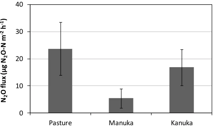
Though not statistically significant, due to low replication (n = 3) (F2,6=1.69;P=0.261), preliminary

experiments indicated a trend showing reduced N2O fluxes from soil planted with manuka (Figure

(43)

0

10 20 30 40

Pasture

Manuka

Kanuka

N

2

O

fl

u

x

(µ

g

N

2

O

-N

m

-2

h

-1

)

Figure 3.10 Preliminary nitrous oxide fluxes (µg N2O-N m-2 h-1) beneath plant species: pasture (P),

manuka (M), kanuka (K) following application of ~200 kg N ha-1_{dairy shed effluent.}

Error bars are standard error of the mean (n = 3).

y = 0.0042x + 0.3192

R² = 0.8045

y = 0.0259x + 0.3192

R² = 0.9982

y = 0.008x + 0.3204

R² = 0.918

y = 0.0125x + 0.3217

R² = 0.9964

0.30

0.35

0.40

0

1

2 N

2

O

c

o

n

cen

tr

at

io

n

(µL

L

-1

)

Time (h)

B

P

M

K

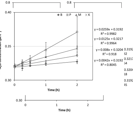
Figure 3.11 Preliminary N2O concentrations (µL L-1) for blank (B), pasture (P), manuka (M), and

kanuka (K) species following application of ~200 kg N ha-1_{dairy shed effluent. Error}

bars are standard error of the mean (n = 3).

3.4.2 N

2

O Fluxes

Examination of raw N2O concentration data showed high variability and a lack of a linear relationship

with the time the samples were taken following chamber closure (Figure 3.12). A large proportion of R2_{values from a linear regression were low (39% were}_≤_{0.3) (Figure 3.13). Thus it was not possible to}