Multi-scale analysis of carbon stocks and process indicators in the agro-ecosystem of Canterbury, New Zealand

(1)

Lincoln

University

Digital

Thesis

Copyright

Statement

The

digital

copy

of

this

thesis

is

protected

by

the

Copyright

Act

1994

(New

Zealand).

This

thesis

may

be

consulted

by

you,

provided

you

comply

with

the

provisions

of

the

Act

and

the

following

conditions

of

use:



you

will

use

the

copy

only

for

the

purposes

of

research

or

private

study



_you

_will

_recognise

_the

_author's

_right

_to

_be

_identified

_as

_the

_author

_of

_the

_thesis

_and

due

acknowledgement

will

be

made

to

the

author

where

appropriate



_you

_will

_obtain

_the

_author's

_permission

_before

_publishing

_any

_material

_from

_the

thesis.

(2)

Multi-scale analysis of carbon stocks and process indicators in the

agro-ecosystem of Canterbury, New Zealand

A thesis

submitted in partial fulfilment

of the requirements for the Degree of

Doctor of Philosophy

at

Lincoln University

by

Johannes Welsch

(3)

ii

Abstract of a thesis submitted in partial fulfilment of the

requirements for the Degree of Doctor of Philosophy

Abstract

Multi-scale analysis of carbon stocks and process indicators in the

agro-ecosystem of Canterbury, New Zealand

by

Johannes Welsch

Increasing interest in characterising carbon dynamics in the agricultural landscape has been driven by the clear need for greenhouse gas mitigation strategies in response to global climate change. However, little quantitative information is available about carbon stocks and processes in agro-ecosystems. Better understanding of carbon stocks and processes is of particular importance in New Zealand, where farmland occupies large areas across the country and ongoing change in farming practices, land management and intensification are affecting carbon stocks and processes and ultimately, agricultural sustainability. This study aimed to quantify and understand variation in above- and below-ground carbon stocks and processes in shelterbelts and paddocks at multiple scales within the agro-ecosystem of

Canterbury, New Zealand. In an initial pilot study across four farms showed that variability in above- and below-ground carbon stocks among-farms was smaller than between shelterbelt and paddocks. Using this knowledge to determine appropriate sampling intensity, I quantified carbon stocks and processes within shelterbelts across 34 farms, focussing particularly on understanding how within-shelterbelt-scale (e.g. soil moisture, pH), shelterbelt-scale (e.g. shelterbelt type, age, and tree biomass), farm-scale (e.g. land use) and landscape-scale (e.g. soil type) factors was related to variability of these variables. Total above- and below-ground carbon pools in shelterbelts were similar for exotic and native shelterbelts (152.6 ± 131 t C ha -1_{and 110.8 ± 128 t C ha}-1_{, respectively [mean ± standard errors]), although native shelterbelts}

(4)

iii and exotic shelterbelts. Most variability in carbon stocks was explained at the shelterbelt scale by shelterbelt type, age and size, whereas farm scale played a minor role and soil type was unimportant. Carbon cycle processes varied primarily at the shelterbelt and paddock level. Leaf litter decomposition and microbial activity were twice as high and invertebrates were more active in native shelterbelts compared to exotic shelterbelts, and variability in these indicators were best explained by within-shelterbelt factors (e.g., soil moisture, pH, organic and labile carbon) and shelterbelt characteristics (age, biomass, and vegetation type). Therefore, above-ground shelterbelt-scale factors drive carbon cycle process indicator rates and biological activity in the Canterbury agro-ecosystem, rather than land use or landscape factors. These field data were used in GIS-based spatial carbon model which expored and evaluated a number of agricultural land use, cover and management scenarios and their impact on soil carbon stocks over the enxt 10 years (2014 – 2024) in combination with quantifying the amount of shelterbelt area needed to offset the potential soil carbon loss. While the model default settings predicted an increase in soil carbon stocks, the literature based alternative scenarios, commonly predicted a decrease of 10%, 6%, 34% in soil carbon stocks in the alternative dairy, sheep and beef and arable scenarios. This study shows that native shelterbelts in agro-ecosystems have considerable potential for increasing carbon pools and enhancing carbon cycle process, particularly as they age through time. Contrary to current assessments, this study was not able to provide definate evidence on the effect of further intensification and land clearing on carbon stocks in Canterbury. Future studies should include long-term investigation of carbon stocks and processes across a wider variety of shelterbelt and farm types.

(5)

iv

Acknowledgements

There are a number of people who made this thesis possible and who deserve a big thank-you. First and foremost are my farmers. They provided the foundation for this work by providing me access to their farms and sharing their thoughts, experience and opinions about my topic. All of them have a very busy lives and, at the same time, they were very open and generous with their time, insight and hospitality. I sincerely enjoyed the opportunity to visit their farms, gain a new insight into rural New Zealand and to see their beautiful farms.

Secondly, the staff and students at Lincoln University who provided time and support in a number of ways; but first of all to my supervisors, Dr. Bradley Case, Dr. Hannah

Buckley, Dr. Niklas Lehto, Dr. Eirian Jones and Dr. Roddy Hale. I really appreciated their guidance, feedback and ongoing encouragement and interest in my topic.

Thirdly, I’d like to thank the Brian Mason – Scientific and Technical Trust, James Bruce-Smith Scholarship and Lincoln University for financial support of my research. The Department of Soil and Physical Sciences at Lincoln and the New Zealand Agricultural Greenhouse Gas Research Centre also provided substantial in-kind support.

The support of a number of people in and around Lincoln University: Sandy, Miles, Candice, Caitriona, Bernadette, Roger, Janette and Crile, with their support with lab

equipment, analysis, and discussions and feedback on earlier versions of the thesis. There were many friends and postgraduate students who also accompanied and helped me along the way – Sarah, Vikki, Mike, Carina, Richard, Meike, Sini, Kate, John, Peter, Kelsey, Nick, Ben, Sophie, Sebastian, Maiki, Kirsty and Brooke, who provided friendship, intellectual

(6)

v

List of Tables

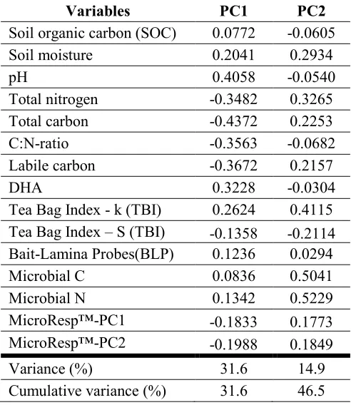
Table 2-1: Summary of general soil, climate and vegetation characteristics of shelterbelts and adjacent paddocks sampled at the four sheep farm study sites, as shown in Figure 2-1. ... 35 Table 2-2: Principal component axis loadings for shelterbelt data and the variance explained. The

table shows the loadings for carbon stocks, carbon cycle processes and soil

characteristic variables. PC scores are shown for each axis. ... 47 Table 2-3: Principal component axis loadings for paddock data and variance explained. The table

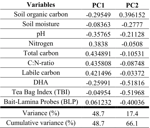
shows the loadings for carbon stocks, carbon cycle processes and soil characteristic variables with the bold PC scores for each axis. ... 49 Table 2-4: Soil carbon stocks and processes across the four farm sites and two cover types

(paddocks and shelterbelts). Samples were collected from paddocks and shelterbelts at each of the farm sites. ANOVA was used to compare means for each cover type (paddock and shelterbelt; df = 1; F-values, P-value) and the differences between the farm sites (A, B, C, D; df = 3; F-values, P-value). Microbial C and N were not

analysed for the paddock sites. Dehydrogenase enzyme activity (DHA). ... 51 Table 2-5: Mean (± standard deviation) soil organic carbon stock (SOC), soil characteristics (pH

and soil moisture) and dehydrogenase enzyme activity (DHA) within paddocks and shelterbelts (total df = 59, treatment df = 2 (excluding DHA; total df = 35, treatment df = 2). The reduced number of variables is due to fewer variables analysed per sample point per site due to cost. ... 53 Table 2-6: Power analysis results for soil carbon stock, soil characteristics and processes, The

table shows the number of samples necessary to have a 80% or 90% chance of

detecting the differences for shelterbelt and paddock site separately. ... 56 Table 3-1: Summary of all farms by land use (beef, crop, dairy and sheep), soil order (G - grey;

B - brown; P - pallic; R - recent), general farm number, shelterbelt type and botanical name of shelterbelt species. The farm code links back to Figure 3-1, a) for their location. ... 69 Table 3-2: Summary of biomass compartments (above-ground tree biomass, coarse-woody

debris, herbaceous biomass, litter, root estimates and soil). This is followed by indicating the different ways each compartment is sampled and which measurements are taken and used for further analysis. ... 72 Table 3-3: Summary of all tree, shrub and plant species in this study, common name, botanical

name, order, family, stem tissue densities over bark (Holdaway et al., 2014) used for analysis and the allometric or total biomass equation references ... 73 Table 3-4: Summary of all multi-model inference models used for analysis with the soil carbon

stocks. The list contains the different candidate models used and the variables within each model are listed. Shelterbelt and paddock model sets differ as the paddock sites did not have above-ground woody vegetation or age of shelterbelt. ... 79 Table 3-5: Summary of all 34 study farms and ordered by shelterbelt type (exotic or native) and

grouped by land use. The farm code (refer to Figure 3-1), and shelterbelt

characteristics are given. Shelterbelt characteristics include age, diameter at breast height (DBH; mean ± one standard deviation (SD)), height, number of rows and spacing of trees. In addition, the soil characteristics, pH and soil moisture, are included for each shelterbelt type as site-level means ± one standard deviation (SD). ... 81 Table 3-6: Model selection results for soil carbon stocks under shelterbelts and a set of candidate

models; models are ranked based on AICc with the most informative mode (lowest AICc) at the top. For each model are a number of parameters shown, including the candidate model names, the number of model parameters (K), the second-order Akaike information criterion (AICc), the distance from the best model (ΔAICc), the Akaike weight (wi), log likelihood (LL), the fixed/marginal effects alone (R2m_{) and the} fixed and random/conditional effects combined (R2C_{); bolded models are within two} AICc of the top model and considered equally informative. ... 90 Table 3-7: Model selection results for soil carbon stocks under paddock and a set of candidate

(10)

ix AICc) at the top. For each model are a number of parameters are shown, including the candidate model names, the number of model parameters (K), the second-order Akaike information criterion (AICc), the distance from the best model (ΔAICc), the Akaike weight (wi), log likelihood (LL), the fixed/marginal effects alone (R2m_{) and the fixed} and random/conditional effects combined (R2C_{); bolded models are within 2 AICc of} the top model and considered equally informative. ... 96 Table 4-1: Summary of carbon cycle process measures, indicating what measurements were taken and used for analysis for each process in shelterbelt and paddocks; ‘X’ indicates where each process was sampled ... 113 Table 4-2: Derivation and description of four scales comprising the hierarchical spatial analysis

framework used in the mixed-effects modelling for shelterbelt and paddock ... 118 Table 4-3: Multi-model inference models used for analysis with the carbon cycle processes in

shelterbelts and paddocks. The list contains the different candidate models used and the variables within each model are listed. Shelterbelt and paddock model sets differ as the paddock sites did not have above-ground woody vegetation effects, such as age or biomass of shelterbelt. ... 121 Table 4-4: Model selection results for above- and below- ground carbon cycle processes

considering above-ground shelterbelt vegetation cover (native and exotic woody vegetation) and a set of candidate models; models are ranked based on AICc with the most informative mode (lowest AICc) at the top. Shown for each model are a number of parameters, including the model names, the number of model parameters (K), the second-order Akaike information criterion (AICc), the distance from the best model (ΔAICc), the Akaike weight (wi), log likelihood (LL) and the regression coefficient of variation (R2_{); bolded models are within two AICc of the top model and are considered} equally informative. Dehydrogenase enzyme activity (DHA), Bait-Lamina Probes (BLP) and Tea Bag Index (TBI). ... 128 Table 4-5: Model selection results for carbon cycle processes in paddocks and a set of candidate

models; models are ranked based on AICc with the most informative mode (lowest AICc) at the top. Shown for each model are a number of parameters including the model names, the number of model parameters (K), the second-order Akaike information criterion (AICc), the distance from the best model (ΔAICc), the Akaike weight (wi), log likelihood (LL) and the regression coefficient of variation (R2_{); bolded} models are within two AICc of the top model and considered equally informative. Dehydrogenase enzyme activity (DHA), Bait-Lamina Probes (BLP), Tea Bag Index (TBI). ... 137 Table 5-1: Summary of land cover types with the assigned factor values and rationale taken

directly from the New Zealand Greenhouse Gas Inventory (MfE, 2013). The factor values express the effect on soil carbon capacity and change for land cover (re-classed LCDB data) ... 152 Table 5-2: Summary of land use classes with factor value and rationale. The land use classes, factor

values and rationale are derived from the New Zealand Greenhouse Gas Inventory (MfE, 2013); The land use factor values express the effect on soil carbon capacity and change

for land use (re-classed Agribase data). 151

Table 5-3: Summary of default values for management and rationale of various land cover types derived from the New Zealand Greenhouse Gas Inventory (MfE, 2013). The factor values express the effect on soil carbon capacity and change for land cover (re-classed LCDB

data). 151

Table 5-4: Summary of different land cover changes and management effects on soil carbon stocks per decade for dairy, sheep and beef and arable farming (‘↔’ no change, ‘↘_{’ decrease and} ‘↗’ increasing effect on soil carbon stock). 154 Table 5-5: Summary of all scenarios for the three farming types (dairy, sheep and beef, arable

farming), a short scenario description and indicating which factor values were used for

land use, land cover and management. 156

(11)

(12)

xi

List of Figures

Figure 1-1: Above- and below-ground carbon stock compartments (left) and carbon cycle

processes (right) in a terrestrial ecosystem ... 22 Figure 2-1: The map shows the four farm sites and main soil types within the Canterbury region.

The green dots show the locations of the four study sites (A, B, C and D). The inset map shows the location of the study area within the South Island of New Zealand. ... 33 Figure 2-2: Bird’s-eye view of the within- shelterbelt and adjacent paddock sampling design for

carbon stocks and processes both above- and below-ground at the farm scale. The transect shows both the shelterbelt and the paddock transects over 100 m at a 25 m distance from the shelterbelt edge. The close up sampling design below shows three sampling rows, the different sample points and the sample types at each point: red dots indicate the sample site for soil carbon, chemistry sample sites; orange circles indicate the Bait-Lamina Probes (BLP) and the Tea Bag experiment sites; dark blue circles indicate total carbon and nitrogen, microbial C and N and MicroResp™ sample points; green circles indicate biomass sample points; the dotted line signifies the shelterbelt centre line. ... 37 Figure 2-3: A comparison of: a) soil moisture (%); and b) pH (mean ± 2 standard errors) across

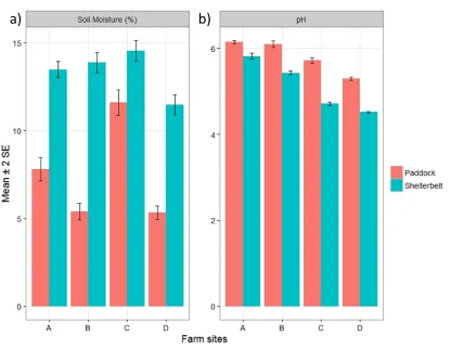
four farm sites (A, B, C and D) between paddocks and shelterbelts (N = 120 for each variable, and N = 30 per farm) ... 45 Figure 2-4: PCA ordination of MicroRespTM_{soil carbon profiling in shelterbelts at the four farm}

sites (A, B, C, D). Points represent the individual sampling points in each shelterbelt (N = 7 plus one bulk sample) (Figure 2-2). Ellipses highlight the centre and dispersion of samples in the ordination space (using the standard error of the weighted average of scores). A further description of the inter-farm site variation is provided in the text. The first and second axes account for 41.4% and 23.7% of the data variation,

respectively. ... 46 Figure 2-5: PCA ordination of carbon stocks, carbon cycle processes and soil characteristic

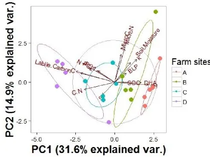
variables in shelterbelts at the four farm sites (A, B, C, D). Points show the clustering of the farm sites and the variables investigated with arrows. Ellipses highlight the 50% centroids and the dispersion of samples in the ordination space. A further description of the variation is provided in the text. The first and second axes account for 36.6% and 17.2% of the variation, respectively... 48 Figure 2-6: PCA ordination plot for carbon stock and carbon cycle process data in paddocks

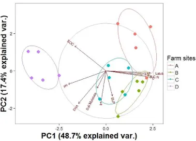
across four study sites (A, B, C, D). Points show the clustering of the farm sites and the variables investigated with arrows. Ellipses highlight the 50% centroids and dispersion of samples in the ordination space. A further description of the variation is provided in the text. The first and second axes account for 48.7% and 17.4% of the variation, respectively. ... 50 Figure 2-7: Mean (± 2 standard errors) soil carbon stocks (a - d) and carbon cycle processes (e - i)

for paddocks and shelterbelts at each of the four farm sites (A, B, C and D). The number of samples per cover type within farm is included in brackets; microbial N and C were not sampled in paddocks. Dehydrogenase enzyme activity (DHA), soil organic carbon (SOC), Tea Bag Index (TBI), Bait-Lamina Probes (BLP). ... 52 Figure 2-8: Mean (± 2 standard errors) soil organic carbon (SOC), soil moisture, pH and

dehydrogenase enzyme activity (DHA) variability between the rows in paddocks and shelterbelts across all four farm sites (A, B, C, D). The four variables were sampled in paddocks and shelterbelts sites in rows 1, 2 and 3 (Figure 2-2). The number of samples per row is included in brackets. ... 54 Figure 3-1: Maps showing: (a) the location and distribution of all 34 farm sites, coloured by land

(13)

xii Figure 3-2: Bird’s-eye view of within shelterbelt and adjacent paddock sampling design for carbon

stock compartments above- and below-ground at the farm scale. The transect shows both the shelterbelt and the paddock transect over 100 m in 25 m distance from the shelterbelt edge; the close up sampling design below shows the different sample points and sample types: red dots are soil carbon samples sites (total-, organic- and labile-carbon) and soil properties (soil moisture and pH); dark blue circles are bulk density, tree dimensions (dbh, height), coarse-woody debris, herbaceous and litter sample sites. ... 71 Figure 3-3: Comparison of carbon stocks (t ha-1 _{± 2 standard error) within native and exotic}

shelterbelts. The carbon stocks were quantified for six ecosystem pools (tree biomass, coarse-woody debris (CWD), herbaceous vegetation, litter, roots, soils and Total), among different shelterbelt types of native and exotic species and four contrasting land use types (crop, beef, dairy, sheep); Data table was added in Appendix B 1. ... 85 Figure 3-4: Comparison of total, organic and labile carbon stocks (mean t ha-1 _{± 2 standard errors)}

between native and exotic shelterbelts and the adjacent paddocks. The soil carbon stocks were quantified across all 34 farms; Data table was added in Appendix B 2. ... 86 Figure 3-5: Variance partitioning of random effects for three soil carbon stocks across four nested

scales in: a) paddocks[black and orange represent within-paddock scales]; b) shelterbelts; c) only native shelterbelts; and d) only exotic shelterbelts (Figure 3-1). The figures shows the random effects for total carbon, soil organic carbon and labile carbon and at which scale the variance resides: soil region scale, farm scale, shelterbelt scale and within-shelterbelt scale. ... 88 Figure 3-6: Model average predicted total soil carbon value (n = 243) for farm types (lines)

coloured by the shelterbelt types (exotic, native) for: a) pH; b) age; c) soil moisture; and d) shelterbelt biomass, as generated from shelterbelt model sets (Table 3-6), including a model-average estimate ± unconditional standard error; points are

observed data coloured for native and exotic shelterbelts. ... 92 Figure 3-7: Model average predicted soil organic carbon (n = 243) for farm types (lines) coloured

by the shelterbelt types (exotic, native) for: a) pH; b) age; c) soil moisture; and d) shelterbelt biomass as generated from shelterbelt model sets (Table 3-6) , including model-average estimate ± unconditional standard error; points are observed data coloured for native and exotic shelterbelts. ... 93 Figure 3-8: Model average predicted labile carbon (n = 243) for farm types (lines) coloured by the

shelterbelt types (exotic, native) for: a) pH; b) age; c) soil moisture; and d) shelterbelt biomass as generated from shelterbelt model sets (Table 3-6), including model-average estimate ± unconditional standard error; points are observed data coloured for native and exotic shelterbelts. ... 94 Figure 3-9: Model average predicted total soil carbon (n = 239) in paddocks under different land

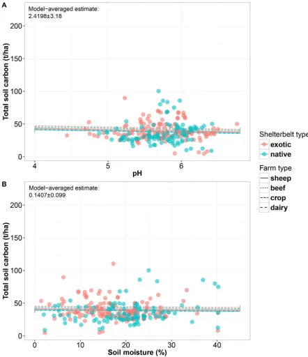
use (lines) for: a) pH; and b) soil moisture in paddocks; generated from paddock model sets (Table 3-7), including model-average estimate ± unconditional standard error. Raw data of paddocks adjacent to native or exotic shelterbelts are shown in green and red, respectively. ... 97 Figure 3-10: Model average predicted soil organic carbon (n = 239) in paddocks under different

land uses (lines) for: a) pH; and b) age of paddock and c) soil moisture, as generated from paddock model sets (Table 3-7), including model-average estimate ±

unconditional standard error. Raw data of paddocks adjacent to native or exotic shelterbelts are shown in green and red, respectively. ... 98 Figure 3-11: Model average predicted labile carbon (n = 239) in paddocks under different land uses (lines) for: a) pH; b) age of paddock; and c) soil moisture, as generated from paddock model sets (Table 3-7), including model-average estimate ± unconditional standard error. Raw data of paddocks adjacent exotic and native shelterbelts are shown in red and green, respectively. ... 99 Figure 4-1: Maps showing: (a) the location and distribution of all 34 farm sites, coloured by land

(14)

xiii represents the Landscape (coarsest) scale and is shown in the map nested within

Canterbury; all 34 farms are nested within the regional scale, as illustrated on the right hand side. ... 110 Figure 4-2: Bird’s-eye view of within-shelterbelt and adjacent paddock sampling design for

carbon stock compartments above- and below-ground at the farm scale. The transect shows both the shelterbelt and the paddock transect over 100 m at a 25 m distance from the shelterbelt edge; the close up sampling design below shows the different sample points, sample types: purple circles indicate leaf litter bags, microbial activity (DHA), microbial community profiling (MicroResp™); the green circle indicates invertebrate activity (BLP) and organic matter decomposition at the Tea Bag Index (TBI) sample point. ... 112 Figure 4-3: PCA ordination of MicroResp™ soil carbon profiling in; a) shelterbelts (N = 168); and

b) paddocks (N = 168). Further description of inter-farm site variation provided in text. The first and second axis account for 41.4% and 23.7% of the data variation, respectively. ... 122 Figure 4-4: Decomposition rate k and stabilisation factor S (± 2 standard errors) from Tea Bag

Index for native and exotic shelterbelt sites (N = 59); k represents short-term dynamics and S is indicative for long-term carbon storage within two different shelterbelt types. ... 123 Figure 4-5: Mean (± 2 standard error) leaf litter residue (%) in shelterbelt for exotic and native leaf litter within exotic and native shelterbelts (N = 177) ... 124 Figure 4-6: Variance partitioning results of random effects for five carbon cycle processes across

four nested scales in a) paddocks [black and orange represent within-paddock scales] and shelterbelts (Figure 3-1, c). The figures shows the random effects for

MicroResp™, Bait-Lamina Probes (BLP), Tea Bag Index (TBI), dehydrogenase enzyme activity (DHA) and leaf litter decomposition and the scales at which the variance resides; landscape scale, farm scale, shelterbelt scale and within-shelterbelt scale. ... 126 Figure 4-7: Model average predicted MicroResp™ value (n = 168) for farm types (lines) coloured

by the shelterbelt types (exotic, native) for: a) soil moisture; b) pH; c) precipitation; d) temperature; e) soil organic carbon; f) labile carbon; g) tree biomass; and h) age of shelterbelt as generated from shelterbelt model sets (Table 4-4), including model-average estimate ± unconditional standard error; points are observed data, coloured by exotic and native shelterbelts. ... 131 Figure 4-8: Model average predicted litter residue value (N = 177) for farm types (lines) coloured

by the shelterbelt types (exotic, native) for: a) soil moisture; b) pH; c) precipitation; d) temperature; e) soil organic carbon; f) labile carbon; g) tree biomass; and h) age of shelterbelt, as generated from shelterbelt model sets (Table 4-4), including model-average estimate ± unconditional standard error; points are observed data, coloured by exotic and native shelterbelts. ... 132 Figure 4-9: Model average predicted Dehydrogenase enzyme activity (DHA) value (N = 235) for

farm types (lines) coloured by the shelterbelt types (exotic, native) for: a) soil moisture; b) pH; c) precipitation; d) temperature; e) soil organic carbon; f) labile carbon; g) tree biomass; and h) age of shelterbelt, as generated from shelterbelt model sets (Table 4-4), including model-average estimate ± unconditional standard error; points are observed data, coloured by exotic and native shelterbelts. ... 133 Figure 4-10: Model average predicted Bait-Lamina Probes (BLP) value (N = 235) for farm types

(lines) coloured by the shelterbelt types (exotic, native) for; a) soil moisture; b) pH; c) precipitation; d) temperature; e) soil organic carbon; f) labile carbon; g) tree biomass; and h) age of shelterbelt as generated from shelterbelt model sets (Table 4-4),

including model-average estimate ± unconditional standard error; points are observed data, coloured by exotic and native shelterbelts. ... 134 Figure 4-11: Model average predicted Tea Bag Index (TBI) value (N = 235) for farm types (lines)

(15)

xiv including model-average estimate ± unconditional standard error; points are observed data, coloured by exotic and native shelterbelts. ... 135 Figure 4-12: Model average predicted MicroResp™ value (N = 168) for farm types (lines) coloured

by the paddock adjacent to shelterbelt types (exotic, native) for: a) soil moisture; b) pH; c) precipitation; d) temperature; e) soil organic carbon; and f) labile carbon as generated from paddock model sets (Table 3-4), including model-average estimate ± unconditional standard error; points are observed data, coloured by paddock adjacent to native and exotic shelterbelts. ... 138 Figure 4-13: Model average predicted Dehydrogenase enzyme activity (DHA)value (N = 245) for

farm types (lines) coloured by the paddock adjacent to shelterbelt types (exotic, native) for: a) soil moisture; b) pH; c) precipitation; d) temperature; e) soil organic carbon; and f) labile carbon as generated from paddock model sets (Table 3-4), including model-average estimate ± unconditional standard error; points are observed data, coloured by paddock adjacent to native and exotic shelterbelts. ... 139 Figure 5-1: Map showing: a) a locator map for the Canterbury region within New Zealand; b) the

location of the case study area within Canterbury ... 150 Figure 5-2: Current soil carbon stocks in 2014 for the case study area from Chapter 3; white areas

(larger water bodies with no information =no carbon stock data available). 155 Figure 5-3: Summary of land use and land cover data for Canterbury for (a) the total area each

land use class occupies (ha) based on Agribase data in 2006 and 2014; and (b) the total area each land cover class occupies (ha) data based on LCDB data in 2001 and 2012, on the Canterbury Plains (500 m a.s.l.) in New Zealand. ... 159 Figure 5-4: Soil carbon stock capacity maps based on land use, cover and management in the

study area for a) 2004 and b) 2014 across Canterbury. The map shows the result of the soil carbon capacity calculations on a scale between decreasing capacity (orange-yellow; 0 to 1), no change (red; 1) and increasing capacity (pink, purple, dark blue; 1-1.3). White areas (larger water bodies or parcels with no information were not

considered in the analysis). ... 161 Figure 5-5: The map shows the change in the trajectory of soil carbon capacity between 2004 and

2014 across Canterbury (Figure 5-4). White areas (larger water bodies or parcels with no information were not considered in the analysis). ... 162 Figure 5-6: Summary of all scenarios (Table 4) and projections of future soil carbon stock changes

(16)

xv

Abbreviations and Acronyms

DoC Department of Conservation

Esri Environmental Systems Research Institute

ETS Emissions Trading Scheme

FAO Food and Agriculture Organisation

GIS Geographic information system

Ha Hectare

MAF Ministry of Agriculture and Forestry

NZ New Zealand

OECD Organisation for Economic Co-operation and Development

NZAGRC New Zealand Agricultural Greenhouse gas Research Centre

IPCC Intergovernmental Panel on Climate Change

DHA Dehydrogenase enzyme activity

BLP Bait-Lamina Probes

TBI Tea Bag Index

C Carbon

N Nitrogen

GHA Greenhouse gas

(17)

16

Chapter 1 Introduction

1.1 Background

Global climate change is one of the most pressing environmental issues worldwide (IPCC, 2007a). Increased greenhouse gas (GHG) concentrations in the atmosphere, particularly the proportion caused by anthropogenic actions, such as deforestation and land clearing for agricultural production, are one of the main causes of accelerated climate change (Crowley, 2000; Houghton, 1999). Carbon dioxide (CO2) is one of the most important GHGs and, in 2004, accounted for 77% of total

anthropogenic GHG emissions (Oliver et al., 2005). While other GHGs, such as CH4,

O3, N2O and NOx, are more potent on a per molecule basis in terms of contribution to

the greenhouse effect, CO2 far exceeds other GHGs in importance due to the large

increase of 40% in its atmospheric concentration in recent decades (Blasing, 2013; Rodhe, 1990). A reduction in the use of fossil fuels should lead to a gradual reduction in atmospheric CO2 concentration (Sterman & Sweeney, 2002). In the meantime,

consideration of other options, such as ways to increase carbon sequestration in vegetation and soils, might provide short-term benefits by reducing the concentration of CO2 in the atmospheric pool (Batjes, 1998; House et al., 2002; UNEP, 2011).

Carbon is stored in four major pools: the atmosphere, biosphere, oceans and sediments. Carbon stored in the forest biomass is also referred to as a carbon sink. Carbon moves from pool to pool by chemical, physical and biological processes. The terrestrial biosphere includes the organic carbon in all land-living organisms, both alive and dead, as well as carbon stored in sediments. Soils are an important

component of the global carbon cycle, holding one of the largest terrestrial pools of carbon. It is estimated to be approximately 1500 Petagrams of carbon (PgC)

(18)

17 removal of natural woody habitat, through vegetation clearance, has played a role in carbon stocks declining in recent decades at a rate of approximately 0.8 GtC year (Schlesinger et al., 2000).

1.2 Historical background of land cover and change

Vegetation clearance and extinction of native flora and fauna has been occurring since c. 1000 years B.P, when New Zealand was settled by Polynesians, which led to the extinction or reduction of much of the vertebrate fauna, destruction of half of the lowland and montane forests, and widespread soil erosion (McGlone 1983; McGlone 1989). The climate and natural vegetation changed over the same time but had negligible effects on the fauna compared with the impact of settlement. The most severe modification occurred between 750 and 500 years ago, when a rapidly

increasing human population, over-exploited animal populations and used fire to clear the land. Human predation, and destruction of forest habitat eliminated the numerous large ground birds. Most forests remaining today are wet mountain land communities, and may never have experienced severe browsing pressure until Europeans introduced browsing mammals (McGlone 1989). Knowledge of these climatic, physical and cultural forces which shaped the biota of present day New Zealand are important for understanding how to manage the remaining estate. However, anthropogenic

modification is just one of many environmental factors: large-scale erosion,

earthquakes, volcanic eruptions, fire, extreme climatic events and long-term climatic trends are all part of the natural background of change. It is difficult to distinguish the effects of these natural changes from those caused by humans. Before people arrived, more than 80% of New Zealand was covered in forest. Māori burnt about 40% of the forest within 200 years of arriving – probably to clear space for gardens, tracks and settlements. Large numbers of Europeans settled in New Zealand after 1840 (Masters, et al. 1957). They cleared much of the remaining lowland forest for farming, and cut down many more large trees for timber. Today less than a quarter of New Zealand is covered in forest and cleared land in hilly areas is prone to erosion.

(19)

18 almost total transformation of the original land cover to a dominance of introduced plant species. The landscape is now dominated by pasture or cropping and lesser extent, by exotic forest plantations. Conversion of these formerly forested landscapes to grassland through Maori and European fires has arguably been one of the most significant human-induced changes to the carbon stocks both above- and below-ground with the almost complete removal of tree biomass resulting in exposed soil (Web, 2008).

Soil is still the largest terrestrial carbon pool but is threatened by ongoing removal of natural woody habitats (Vashum & Jayakumar, 2012). It is known that woody vegetation features in agro-ecosystems can act to mitigate lost or impaired ecosystem services (Bullock et al., 2001). These woody vegetation features, or ‘non-production’ uses of land, (Seabrook et al., 2008; Welsch et al., 2014) such as shelterbelts,

hedgerows, riparian strips and road-side plantings, have been shown to serve

numerous functions (Brandle et al., 2004; Marshall & Moonen, 2002), including the provision of essential habitats for a range of taxa (Mize et al., 2008), sequestration and storage of carbon (Czerepowicz et al., 2012; Nair et al., 2009), and enhancement of biodiversity and ecological functions (Devictor & Jiguet, 2007; Gurr et al., 2003; Kramer et al., 2011).

1.3 New Zealand agricultural landscapes

Growing sufficient food for an ever growing world population is one of the major challenges of the 21st_{century (Godfray et al., 2010). This challenge is}

accompanied by the concomitant increasing challenge of mitigating or reversing environmental damage and biodiversity loss (Godfray et al., 2010; Godfray & Garnett, 2014). Paradoxically, land use change and intensification to increase production is increasingly being perceived as one of the solutions to the issue, both globally and in New Zealand (Allan et al., 2015; Green & Clarkson, 2005; Phalan et al., 2011).

(20)

19 agro-ecosystem result from biogeochemical cycle changes (i.e. nitrogen and

phosphorus) the hydrological cycle (i.e. irrigation, change of land cover) and species habitat (i.e. clearing of shelterbelts). These listed changes, in turn, affect the

ecosystem and carbon cycle processes (i.e. decomposition, nutrient cycling and mineralisation).

The favourable temperate climate, the abundance of agricultural land and the unique farming practices used in New Zealand facilitate the use of year-round extensive outdoor grazing systems (MfE, 2010). New Zealand has 14.4 million ha of agricultural and cultivated land (StatisticsNZ, 2012) covering approximately 53% of its total area. Since 1990, there have been changes in the proportions of the main livestock species farmed in New Zealand as the profitability of dairy products has become relatively high compared with sheep and beef products. Pastoral land used for dairy has increased, and pastoral land used for sheep and, to a lesser extent, beef has decreased (MfE, 2013). At the same time, land cover such as shelterbelts and woody native remnants has been decreasing as part of the change in livestock type and the accompanying farm management activities (Welsch et al., 2014). This change in land cover, and the clearing of shelterbelts and other woody vegetation covers, has reduced the potential to improve environmental performance by, for example, carbon storage in trees and soil carbon sequestration. These woody vegetation features are important for terrestrial ecosystems and are major components of carbon sequestration strategies (Millward & Sabir, 2011). Time series analysis of satellite data since 1970 and aerial photography since the early part of the twentieth century provide insigts into how land use and land cover have changed. Most of the change happen slowly and on

individual parcels of land, which makes it difficult to detect overall landscape change and its impact on carbon in woody vegetation and soil with the human eye. Therefore, photographic time series analysis of satelite images can at least provide insights into the change of land cover over time.

(21)

20 behind; for example, the agricultural sector contributed around 50% to New Zealand’s greenhouse gas emissions (MfE, 2013).

1.4 Carbon stocks and processes

Soil carbon sequestration is considered an important strategy to offset growing emissions from agricultural industries (Lal, 2004b; Nair et al., 2010; Rees et al., 2005). Farm soil carbon pools account for a significant fraction of global carbon storage (Cole et al., 1993) and play an important role in reducing carbon emissions. This has arisen because of the need to sequester carbon to overcome global climate change (Paustian et al., 1998), and to improve soil quality, as we develop more sustainable and land management practices (Carter, 2002).

However, many variables can affect the dynamics of soil carbon. Studies have demonstrated that climate change may lead to soil degradation and losses in crop and pasture production (IPCC, 2007b). Aside from climate change, land use management practices can also affect soil carbon storage (Post & Kwon, 2000). Soil carbon stocks decline after land use changes from pasture to plantation (−10%), native forest to plantation (−13%), native forest to crop (−42%), and pasture to crop (−59%) (Guo and Gifford 2002). Because of soil carbon’s sensitivity to management (Lal, 2004a) global farmland has lost a large amount of carbon as a result of cultivation and tilling.

The carbon cycle is dependent on climatic factors (i.e. seasons, precipitation and temperature), soil fertility, carbon dioxide concentrations in the atmosphere and the functional traits of plants (i.e. leaf area) (Chapin et al., 2002). These factors determine the rates of photosynthesis and biomass production. Decomposition and respiration rates influence the ability of an ecosystem to accumulate biomass, including carbon. Decomposition rates are influenced by the climate and soil environment (climate variables, and soil variables including pH, chemistry, texture and parent material), woody and leaf litter quality (chemistry and palatability to decomposer organisms) and the decomposer community itself (biomass and specificity) (Strickland et al., 2009; Swift et al., 1981; Wardle & Lavelle, 1997). Respiration rates are determined by photosynthesis and decomposition rates, with an additional consideration of herbivore interactions (Bardgett et al., 1998). Figure 1-1 summarises the major carbon cycle processes in a terrestrial ecosystem.

(22)

21 The majority of carbon released occurs through leaf litter fall and root exudation leading to increases in soil organic matter (SOM) (Chapin et al., 2002). Litter is decomposed by microorganisms in the soil. Again, a large proportion is respired and the rest is converted to less decomposable fractions (i.e. humus). Some of the soil carbon is leached from the ecosystem, or transferred through erosion or disturbance by animals.

(23)

(24)

23 native shelterbelt species, for carbon storage and carbon cycle processes, is less clear. The common perception is that using native species for shelterbelts is not effective due to different growth rates and maintenance demands during the establishment phase. Therefore, efforts were directed towards faster growing, less time demanding species for shelter. These assumptions arose primarily from anecdotal stories within the farming community. At the same time, native shelterbelts may be able to provide more than just carbon storage, through multi-aged species and habitat to native flora and fauna within the agro-ecosystem (Anton et al., 2015; Cierrad et al., 2015). Kirby and Potvin (2007) noted that it is not only the amount of carbon sequestered above-ground that is important, but also the below-above-ground soil carbon stocks, processes and biodiversity benefits.

Carbon estimates in the agricultural landscape have been carried out around the world at various scales using a range of methods. At the global scale, pre-existing national and region soil carbon inventory data are compiled and used to estimate above- and below-ground live plant carbon storage, or biomass estimates, which are used to determine overall carbon stocks in agricultural landscapes (Berenguer et al., 2014; Buringh, 1984; Falloon et al., 2009; Parvia et al., 2012). At the national scales, above- and below-ground carbon estimates in paddocks, shelterbelts, or native remnants may be based on compilations of data from representative inventory sites used in combination with few local field-based sample plots (Baah-Achemfour et al., 2014; Carswell et al., 2012; Garcia-Palacios et al., 2013; Holdaway et al., 2010; Mason et al., 2012). Regional and local scale carbon inventories are usually based merely on individual plots or low number of representative study sites (Berenguer et al., 2014; Kelliher et al., 2014; Sauer et al., 2007).

There is a certain amount of variability present in every scale and

(25)

24 accurate predictions of carbon can be made at the various scales that account for the inherent variation across scales (Bennett et al., 2006; Cumming & Spiesman, 2006; Kivinen et al., 2007; Ricketts et al., 2008). However, drivers for local variability are poorly understood and information at the landscape scale in a highly heterogeneous, complex and interacting agricultural landscape is lacking (Ekbom et al., 2000; Meehan et al., 2013; Wickings et al., 2016). Research on farms has commonly focused on the production area rather than on non-production land with woody

vegetation cover. This begs the question: is there a difference between production and non-production soils on farms and what role does the above-ground cover (shelterbelt or pasture/crop), land use or management play?

Furthermore, researchers have recognised that the actions of individual farmers can have far-reaching impacts at the local and, even, regional scale

(Schellhorn et al., 2008). This shows the necessity of connecting the biophysical and spatial science throughout the landscape, rather than just at the individual property, is necessary. Future studies of ecosystem services and functions (such as carbon

storage) should embrace a broad range of scales and systems, if the generality of these relationships is to be understood.

Previous studies, looking into spatial variation of carbon in above-ground woody biomass, primarily in forests, have shown that the biomass and carbon contents of these pools are influenced by various factors, including climate,

(26)

25

1.6 Research aim and objectives

This thesis aims to quantify and understand variation in above- and below-ground carbon stocks and processes in shelterbelts and paddocks at multiple scales within an agro-ecosystem.

The research had the following objectives:

1. Characterise and quantify variability of soil carbon stock and process

measures at fine scales, within-shelterbelt, paddocks and farms to determine an adequate sampling approach.

2. Identify key spatial scales at which above- and below-ground carbon stock and process measures vary within the agro-ecosystem.

3. Characterise possible drivers of variability in carbon stock and process measures across an agro-ecosystem at multiple spatial scales, including shelterbelt- (species, age, and biomass), farm- (land use) and landscape scale (soil type, climate).

4. Quantify the potential spatial effect of land use, change and intensification on soil carbon stocks across an agro-ecosystem over time, including historical land use and cover change (2004 - 2014) and the potential effects of land use change on soil carbon stocks into the future (2014 - 2024).

1.7 Thesis structure

To address the above research objectives, the reminder of this thesis will cover the following topics:

(27)

26 Furthermore, the optimal spatial sampling intensity for these stocks and processes are determined. The results from this analysis directly inform the sampling design for the landscape scale study in the next two chapters (Chapter 3 and Chapter 4).

In the following two chapters, I quantified the differences in above- and below-ground carbon stocks (Chapter 3) and processes (Chapter 4) among

shelterbelt types and adjacent paddocks to investigate at what scale stock and process indicators vary and which factors explain the variation at multiple scales. Both chapters are based on extensive field data collection. The scales range from within-shelterbelt and paddock factors, to landscape factors. I use variance partitioning to identify the key scales at which carbon stock and process indicators vary and apply mixed effects models to determine; first, the drivers of soil carbon stock variability (Chapter 3) and; second, apply a mixed effects model to determine the drivers of variability in process indicators including the soil carbon stocks as explanatory variables (Chapter 4). The aim of both chapters is to provide a general indication of which factors are driving carbon stock and process indicators within the

agro-ecosystem and at which scale.

In Chapter 5, I assess historical land use and cover change effects on the soil carbon stock capacity (2004-2014) and explore and evaluate a number of agriculture land use and management scenarios and their impact on soil carbon stocks over the next 10 years (2014 – 2024) in combination with quantifying the amount of

(28)

27 using spatial analysis, as well as the opportunities shelterbelts can provide to improve the agro-ecosystem.

(29)

28

Chapter 2 Variability in soil carbon stocks and key carbon cycle

processes at fine scales in the agro-ecosystem

2.1 Introduction

Soil carbon stocks and processes present at any particular location are a result of trade-offs between inputs of organic matter from plant biomass or leaf material deposited and losses of soil carbon due to soil respiration, erosion or leaching. This balance is affected by a series of complex interactions between plant growth, climate, soil type, topography, land use and farm management (Baldock & Skjemstad, 1999). These factors affect soil carbon quantities and cycling process rates on a range of different temporal and spatial scales ranging from plant/shelterbelt scale (0.1 mm – 100 m), to farm scale (20 m – km) and to landscape scale (> km) (Bird et al., 2001). The relative importance of both natural and anthropocentric factors varies at different spatial scales, and the resulting spatial patterns and drivers for carbon stocks and processes are still poorly understood (Doetterl et al., 2015; Vasenev et al., 2015).

Defining the spatial scales at which soil carbon stocks and processes are investigated is critical within the agro-ecosystem, as they have been studied at different scales (mm, cm, m and km). Indeed, a review of different methods for assessing variability and agro-ecosystems indicates the need for more emphasis on spatial scale in such studies (Payraudeau & Van der Werf, 2005). Common scales range commonly from the individual sample point measured with a soil corer

(approximately 28 cm2_{), several sample points are the within-shelterbelt scale (0.01-1}

ha) as well as within-paddock scale (0.01-10ha), farm scale consists of multiple paddocks and shelterbelts (10-1000 ha) and the landscape scale is made up of multiple farms (> 1000 ha). The spatial geography of agriculture requires attention to the appropriate scale (Fahrig et al., 2011), including above- and below-ground as part of these scales. Research has shown that agro-ecology studies across the landscape should not only focus on the field or shelterbelt scale and dynamics of spatial

(30)

29 1984). Across scales, spatial variability of stocks and processes have been found to be influenced by numerous factors, including land use, soil carbon content, topography, above-ground plant cover (pasture vs. woody vegetation; or size, spacing, age), substrate hotspots and fine roots (Banfield et al., 2002; Conant et al., 2003; D’Acunto et al., 2014; Ettema & Wardle, 2002; Li et al., 2016; Schöning et al., 2006). Assessing the spatial variability of carbon stocks and processes within a site and between

different sites will help develop better sampling strategies of these above-ground biota and abiotic properties as well as soil properties and carbon stock (Conant & Paustian, 2002; Ettema & Wardle, 2002; Singh et al., 2010). This highlights the importance of determining spatial variability of these stocks and processes in farm environments (i.e. paddocks and shelterbelts), even within small areas, in order to obtain meaningful results for soil carbon and microbial properties.

In New Zealand, soils under pasture and shelterbelts are important for both extensive and intensive livestock farming. While there is a growing body of evidence about above-ground carbon stocks and variability in shelterbelts, both internationally and in New Zealand (Bangura et al., 2015; Czerepowicz et al., 2012; Hawke et al., 1999; Sauer et al., 2007), the same cannot be said for agricultural soils. Agricultural soils play a key role in the mitigation of climate change and the provision of a range of ecosystem services that includes the sequestration of carbon (Kort & Turnock, 1998; Mize et al., 2008). Despite growing interest in both above- and below-ground carbon stocks and processes in agricultural soils in recent times, little information is available on the soil carbon stocks and processes in the New Zealand agricultural landscape. There are studies investigating soil carbon at a local (Kelliher et al., 2014), land use specific (Schipper et al., 2007), or smaller regional scale (Parfitt et al., 2013; Schipper et al., 2012; Schipper et al., 2014). The issue is the stocks and processes measurements and their level of variability due to different soil depth increments, sampling intensity, seasonality, different environmental conditions, and analytical approaches.

2.1.1 Soil carbon stocks, processes and measures

(31)

30 2008; Trumbore, 2006; Trumbore et al., 1995). The organic pool is estimated to be as twice as large as the inorganic stocks and amounts to ~1500 Gt C within the top 1 m in the soil profile (Batjes, 1996). Another soil C pool is the labile pool (Labile Carbon), which can also be chemically labile, or biologically labile, neither or both. For the former, it will depend on the other reactants (e.g. reactive with 0.1 M H2O2)

and, for the latter, it is likely to vary with organisms (different microbes will find different parts of the organic matter easier to consume – more labile (Dalal & Chan, 2001)). Several studies have been carried out to estimate how these soil carbon stocks vary in relation to soil properties, land use and climate (Banfield et al., 2002; Conant et al., 2003; Doblas-Miranda et al., 2013; Parras-Alcantára et al., 2015). While these studies frequently refer to ‘variability’ they ultimately describe the increasing or decreasing effects on a particular carbon stock in different soil types (Perruchoud et al., 2000; Zhang & Shao, 2014), land use (Don et al., 2011; Don et al., 2007), or topography (Parras-Alcantára et al., 2015). There is limited evidence that examines the variability of these stocks at a different scales within the same agricultural

landscape (Kelliher et al., 2014; Sauer et al., 2007; Schipper et al., 2014; Schöning et al., 2006; Singh et al., 2010).

A central component of the carbon cycle is the microbial community. This is considered to be the driver for many soil processes, and it plays a key role in

(32)

31 MicroResp™) to estimate the metabolicpotential of microbial communities to use carbon substrates (Campbell et al., 2003; Smalla et al., 1998). Dehydrogenase enzymes are generally present in the topsoil and are essential components of the respiratory enzyme systems of soil microorganisms. Dehydrogenase activity (DHA) can, therefore, be used as an indicator of biological redox systems and a measure of microbial activity in the soil (Wolińska & Stępniewska, 2012). While all the indicator measures discussed have been applied individually, or in some smaller combinations in the past (Burton et al., 2010; Creamer, Stone, et al., 2016; Littlejohn et al., 2015; Simpson et al., 2012; Subhani et al., 2001), no attempt has been made, so far, to combine them to produce a clear picture of how these process indicators vary across scales.

2.1.2 Sampling design and scales

Soil carbon stocks and processes are highly variability at the fine scale (Houghton, 2003; Jian-Bing et al., 2006; Toodd-Brown et al., 2013). This means that we need to know about the nature of this fine-scale variability in order to: 1) develop appropriate sampling designs for quantifying carbon; and 2) to quantify (scale up) the carbon to larger scales with a known level of certainty. The ability to make inferences about soil carbon stocks and processes is compromised at any scale without an

appropriate sampling design and sample size to account for the variability (Allen et al., 2010). Results from a recent small-scale study on carbon stock variability on two farms showed clear differences in soil carbon stocks between them (Appendix A). The study found that different soil carbon measures were able to detect differences between locations (paddocks and shelterbelts) and land management, based on the sampling design and intensity. Evidence from Bangura et al. (2015) supported the sampling design and sample number in this small-scale variability study based on investigations of soil carbon sequestration in agro-forestry systems in Australia. This study provided the first indicative approach for a clear sampling approach to assess spatial variability of carbon stocks and processes within farms and across

heterogeneous agricultural landscapes.

(33)

32 related to carbon cycling in the soil. Several recent studies have started to unravel the spatial variability in soil carbon stocks at point, and on field or farm level scale, in a range of natural and modified environments (Bangura et al., 2015; Don et al., 2007; Follain et al., 2007; Schöning et al., 2006). The carbon stock results at field or farm levels are site specific and are difficult to extrapolate or transfer to other sites or to larger scales. At the other extreme, some studies focussed on the estimation of carbon stocks on a national or global scale (i.e. Bhatti et al., 2002; Tan et al., 2004; Vejre et al., 2003). Such estimates rely on a large landscape scale, national or worldwide soil maps, and are based on a small number of soil profiles. Until recently, there were few studies that had used a large number of direct measurements at the landscape or farm scale (Banfield et al., 2002; Grueneberg et al., 2010; Kulmatiski et al., 2004;

Perruchoud et al., 2000). Average carbon stock and process estimates, appropriate for larger scales and national scale modelling, are inadequate for capturing this variability at a local scale.

2.1.3 Aim and objectives

The aim of this chapter was to characterise the variability in soil carbon stocks and key carbon cycle process indicators, both at a fine scale (within shelterbelts and paddocks) and among different sites (farms).

Therefore, the objectives of this chapter were:

1. Assess the ability of different measures to detect spatial differences in soil carbon stocks and carbon cycle processes.

2. Quantify the variability of soil carbon stocks and carbon cycle process indicators between farms, cover types (shelterbelt and paddock) and at different sampling intensities.

(34)

33

2.2 Methods

2.2.1 Study sites

The study was conducted at four sites on the Canterbury Plains, New Zealand (Figure 2-1 and Table 2-1). All four farms sampled in this study had very similar land use histories - low intensive sheep farming for at least 20 years - and all four study sites were made up of a regularly-trimmed pine shelterbelt (Pinus radiata) in the adjacent paddock. Pine shelterbelts were selected because this species is commonly planted widely across Canterbury. The undisturbed soil under the shelterbelt was, typically, covered by 20 cm thick pine needle layer. All shelterbelts studied were oriented N-S or NE-SW, which are the predominant wind directions crop and stock need shelter from. The four study sites were selected for this variability study because they were located on brown, gley, recent and pallic soil types, as these soil types comprise approximately 80% of all agricultural soils types in Canterbury (Figure 2-1).

Figure 2-1: The map shows the four farm sites and main soil types within the

(35)

34 The most prominent soil type, brown soils, have a brown or yellow-brown subsoil below a dark grey-brown topsoil. The brown colour is caused by thin coatings of iron oxides weathered from the parent material which contirbutes to its carbon storage capabilities. Gley Soils are strongly affected by waterlogging and have been chemically reduced. They have light grey subsoils, usually with reddish brown or brown mottles. The grey colours usually extend to more than 100 cm depth.

Waterlogging occurs in winter and spring, and some soils remain wet all year. This soil type has common segregated iron and manganese oxide mottles, concretions or nodules. Organic matter content is usually high. Recent Soils are weakly developed, showing limited signs of soil-forming processes. A distinct topsoil is present but a B horizon is either absent or only weakly expressed. Pallic Soils have pale coloured subsoils, due to low contents of iron oxides. The soils have weak structure and high density in subsurface horizons. Pallic Soils are dry in summer and wet in winter. This soil type has medium to high nutrient content ( except for sulphur), high base

(36)

35

Table 2-1: Summary of general soil, climate and vegetation characteristics of shelterbelts and adjacent paddocks sampled at the four sheep farm study sites, as shown in Figure 2-1.

Farm site Soil order Shelterbelt age _(years) Height _(m) Shelterbelt width (m)

Average

annual rainfall pH ± SD Soil moisture (% ± SD)

A Shelterbelt Brown soil _(B) 18 6 2.5 1000 mm 5.8 ± 0.3 11.5 ± 1.8

Paddock 6.1 ± 0.1 5.8 ± 2.5

B Shelterbelt _Paddock Brown soil _(B) 25 6 2.5 650 mm 6.2 ± 0.2 _{6.1 ± 0.3} 11.8 ± 2.1 _{3.4 ± 1.8}

C Shelterbelt Recent soil _(R) 60 15 4.5 633 mm 4.7 ± 0.1 12.5 ± 2.2

Paddock 5.7 ± 0.2 9.6 ± 2.2

(37)

36 2.2.2 Field sampling and processing

To achieve precise estimates of the paddock and shelterbelt variability, a sampling design that controlled for two important sources of variation (shelterbelt species and land use) was used (Table 2-1 and Figure 2-2). Shelterbelt species and land use were controlled to limit the sampling effort and replication necessary to assess the magnitude of the likely variation. The sampling was done in early summer over the first two weeks in December. The studyassessed the variability along three parallel 120 m transects within each shelterbelt, as well as in three companion transects in the adjacent paddock that ran parallel to, but 25 m from, each shelterbelt edge. The three transects were located within each shelterbelt, centred approximately on the shelterbelt’s midpoint (Figure 2-2). The transects were spaced at even intervals within 50 cm of the edges of the shelterbelt to ensure that the samples collected were representative of the processes within the shelterbelt. Samples were taken at 20 m intervals (from one red point to another). The red dots signified the sample points for organic soil carbon, soil

(38)