Article
1
Evaluation of Analysis by Cross-Validation.
2
Part I: Using Verification Metrics
3
Richard Ménard 1* and Martin Deshaies-Jacques 1
4
1 Air Quality Research Division, Environment and Climate Change Canada; [email protected]
5
* Correspondence: [email protected]; Tel.: +1-514-421-4613,
6
2121 Transcanada Highway, Dorval, (QC), CANADA, H9P 1J3
7
8
Abstract: We examine how passive and active observations are useful to evaluate an air quality
9
analysis. By leaving out observations from the analysis, we form passive observations, and the
10
observations used in the analysis are called active observations. We evaluated the surface air quality
11
analysis of O3 and PM2.5 against passive and active observations using standard model verification
12
metrics such as bias, fractional bias, fraction of correct within a factor 2, correlation and variance. The
13
results show that verification of analyses against active observations always give an overestimation of
14
the correlation and variance. Evaluation against passive or any independent observations display a
15
minimum variance and maximum correlation as we vary the observation weight, thus providing a
16
mean to obtain the optimal observation weight. For the time and dates considered, the correlation
17
between (independent) observations and the model is 0.55 for O3 and 0.3 for PM2.5 and for the analysis,
18
with optimal observation weight, increases to 0.74 for O3 and 0.54 for PM2.5. We show that bias can be
19
a misleading measure of evaluation and recommend the use of a fractional bias such as the modified
20
normalized mean bias (MNMB). An evaluation of the model bias and variance as a function of model
21
values also show a clear linear dependence with the model values for both O3 and PM2.5.
22
Keywords: chemical data assimilation; air quality model diagnostics; cross-validation
23
24
1. Introduction
25
Since 2003, Environment and Climate Change Canada (ECCC) has been producing hourly surface
26
analyses of pollutants covering North America [1, 2] which became operational products in February
27
2013 [3]. The analyses are produced using an optimum interpolation scheme that combines the
28
operational air quality forecast model GEM-MACH output [4] (CHRONOS model output was used prior
29
to 2010 [5]) with real-time hourly observations of O3, PM2.5, PM10, NO2, and SO2 from the AirNow gateway
30
with additional observations from Canada. As those surface analyses are not used to initialize an air
31
quality model, it raises the issue on how to evaluate them. We conduct routine evaluations using the
32
same set of observations as those used to produce the analysis. Once in a while, when there is a change
33
in the system, a more thorough evaluation is conducted where we leave out a certain fraction of the
34
observations and use them as independent observations, a process known as cross-validation.
35
Observations used in producing the analysis are called active observations while those not used for
36
evaluation are passive observations. The purpose of this two-parts paper is to examine the relative merit
37
of using active or passive observations (or independent observations in general) viewed from different
38
evaluation metrics, but also to develop, in Part II, a mathematical framework to estimate the analysis
39
error, and in doing so, to improve the analysis.
40
The evaluation of an analysis is important, even in the case where it is used to initialize an air quality
41
forecast model, since the evaluation of the resulting air quality forecast may not be a good measure of
42
the quality of the analysis. In air quality forecasting, the forecast error growth is small, depicts little
43
sensitivity to initial conditions and is in fact more sensitive to numerous modeling errors such as:
44
photochemistry, clouds, meteorology, boundary conditions and emissions just to name a few [ 6, 7 , 8,
45
9, 10]. Furthermore, chemical species that are observed are incomplete compared to species needed to
46
initialize an air quality model; incomplete in terms of the number of species observed as well as in their
47
kind [ 6, 8, 10, 11]. Only a fraction of the observed species (either of secondary or primary pollutants) are
48
usable for data assimilation, important chemical mechanisms are left completely unobserved and for
49
aerosols, information on size distribution is quite limited and almost inexistent when it comes to
50
speciation [6,10]. Also, the observational coverage is limited to the surface or to total column
51
measurements which, up until now, were available at one or two local times per day. There are thus
52
many assumptions to be made from an analysis to a proper 3D initial chemical condition and surface
53
emission correction and its subsequent impact on the air quality forecast. These considerations warrant
54
an independent evaluation of the quality of the analysis on its own [12].
55
Evaluating an analysis with observations is quite different from evaluating a model with
56
observations, since analyses are created from observations. From a statistical point of view, the
57
observation and analysis cannot be considered independent. However, if we assume that observation
58
errors are spatially uncorrelated. Then, since the passive and active observation sites are never
59
collocated, then the errors from passive observations are uncorrelated with errors of active observations;
60
observations that are used for the analysis. And since the modelling errors is usually assumed to be
61
uncorrelated with observation errors, then it is also uncorrelated with the analysis errors.
Cross-62
validation thus offers a mean to evaluate analyses with statistically independent (passive) observations
63
[13].
64
In this paper, Part I, we evaluate the relative merit of passive and active observations in the
65
evaluation of analyses using standard metrics used for model evaluation. We show how and when the
66
use of active observations can be misleading and that passive observations can provide a mean to identify
67
optimal analyses. Our examples show that optimal analyses, at the independent observation sites, have
68
much smaller biases than the model biases and increase the correlation coefficient by nearly a factor 2.
69
The paper is thus organized as follows. First we present the analysis scheme we will be using, as
70
well as the cross-validation design, the evaluation metrics and the configuration of the experiments.
71
Then in §3, we assess the quality of the analyses in both active and passive observation spaces using
72
standard air quality evaluation metrics, identify some pitfalls of some metrics and advocate using active
73
observations. Conclusions are presented in §4.
74
2. Experimental design
75
2.1. Design of the objective analysis solver
76
In optimum interpolation there is no use of an explicit interpolation observation operator. The
77
correlation between a pair of locations, either from two observations sites or from an observation site to
78
a model grid point, is computed as a function of distance using a prescribed correlation function. The
79
observation operator is in effect a delta function applied over a continuous spatial domain [14].
80
In this study we interpolate the gridded analysis field to observations locations, using bilinear
81
interpolation, to compute residuals such as observation-minus-analysis. Thus there can be a
82
discrepancy between the observation operator used to generate the analysis, i.e. delta functions, and the
83
observation operator used to interpolate the analysis field at the observation location, i.e. bilinear
84
interpolation. To eliminate this discrepancy in observation operators we have revised the optimum
85
interpolation scheme to use explicitly the same bilinear interpolation in handling the error covariance.
86
As in the operational optimum interpolation, the inversion of the innovation covariance matrix for
88
the analysis solver is done using Choleski decomposition on the full matrix. The number of observations
89
to be processed per analysis being of the order of a thousand or less, there was no need for computational
90
simplification for large number of observations by using either data selection [15] or compact support
91
correlation functions [14, 16]. Thus, the analysis scheme used in this study computes explicitly the gain
92
matrix K~ as,
93
1
) ~ ~ ( ~
~
R H B H H B
K T T , (1)
94
where H is a bilinear interpolation operator, B~ is the prescribed background error covariance and R~
95
is the prescribed observation error covariance. The tilde (~ ) emphasizes that these are prescribed,
96
potentially suboptimal, quantities.
97
The computational demand of the Kalman gain was kept low by computing the background error
98
correlation function only at model grid points needed for the bilinear interpolation. For example, to
99
calculate the correlation between a pair of observations requires the computation of correlation between
100
four points surrounding observation 1 (needed for the bilinear interpolation) and the other four points
101
surrounding observation 2, thus forming a 44 correlation matrix Cbetween the target model grid
102
points. Then we calculate HCHT which gives the correlation between two observation sites. This
103
procedure is generalized for the N observations needed for the analysis. Equation (1) also involves
104
the computation of B~HTthat we compute as a set of N representers (i.e. columns of B~HT), each being
105
a 2D field that maps the background error covariance in model space with a single observation location,
106
using again the bilinear interpolation approach to get a single interpolated representor for each
107
observation location. By doing so we keep the consistency between the observation operators used for
108
interpolation of a field and the observation operator used to manipulate matrices.
109
2.2. Cross-validation
110
Cross-validation is a technique to evaluate an analysis (or in general any model that depends on
111
observations) by partitioning the original observation data set into a training set, used to create the
112
analysis, and an independent (or passive) set, used to evaluate the analysis. The most common
cross-113
validation designs are: the k-fold cross-validation, where the original observation data set is partitioned
114
into k equal size subsamples and the leave-one-out cross-validation, where N subsamples are created,
115
each with one different observation set aside for the evaluation while the other N1 observations are
116
used in producing the analysis. The cross-validation is then repeated with all the different sets until all
117
observations have been used for evaluation. Clearly, there are k analyses computed in the k-fold
cross-118
validation and N in the leave-one-out cross-validation, the later being computationally demanding when
119
N is large. The main disadvantage of the k-fold cross-validation is that the analyses being evaluated
120
uses a smaller number of observations (actually(k1)N/k) than the original observation data set,
121
whereas the leave-one-out cross-validation evaluates analysis that uses nearly the same number of
122
observations (actuallyN1) as the original observation data set. This actually matters with the k-fold
123
cross-validation if we need an estimate of the analysis error variance (or any other second moments) as
124
the analysis error variance depends on the number of observations used.
125
Let Ojbe a vector that contains the jth set of observations used for evaluation, and let A(j) be a
126
vector of analysis value interpolated at the verification observation locations of Oj and where the
127
analysis used all observations except those in Oj (the index in parenthesis, i.e. (j), indicates all sets
128
except the set j). It is customary in cross-validation literature (e.g. [17]) to construct a mean square error
129
) (
) (
CV () j (j)
j
T j
j A O A
O
, (2)
131
that represents a misfit quadratic error of the model A- in our case the analysis. Different model A
132
can be compared and selected from which the CV value is smallest. Likewise, a tunable parameter in
133
A can be obtained by minimizing the cost function CV with respect to that parameter. As we shall
134
discuss later in this paper, in §4 and onwards, the bias of (OjA(j)) needs to be removed from the cost
135
function in order to estimate the input error covariance parameters.
136
In applications and thus in all experiments that follows, the analyses and verification against passive
137
observations are made only with a set of observations that has passed a quality control. The quality
138
control is nearly identical to the quality control used for the operational implementation of the analysis
139
of surface pollutants at ECCC (Robichaud et al. [3], supplementary material 1). It consists in discarding
140
observations that report a negative value, or whose value exceeds a certain unrealistic threshold set to
141
300 ppbv for ozone (300 μg/m3 for PM2.5). Observations are also discarded based on innovations (or
142
observed-minus-background values) when, for ozone, they exceed 50 ppbv (100 μg/m3 for PM2.5) in
143
absolute value. The quality-controlled observations are then separated into 3 sets of observations of
144
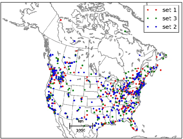
equal numbers, i.e. a 3-fold cross-validation procedure, as illustrated in Figure 1.
145
146
147
148
149
150
151
152
153
154
155
156
157
158
159
160
161
Figure 1. Spatial distribution of the 3 subsets of PM2.5 observations used for cross-validation.
162
The selection algorithm is based on regular picking of station by ID number.
163
The selection into three sets is made by station ID number, selecting on a regular basis each fourth station,
164
starting with station 1 for the first set, station 2 for the second set and station 3 for the third set, and
165
resulting in locally spatially random distribution of each sets of stations. The cross-validation is then
166
made by leaving one set out of the three sets, and using the remaining two sets to produce the analysis.
167
168
2.3. Verification metrics
169
We will evaluate the analyses against passive and active observations with the following standard
170
evaluation metrics used for air quality models [ 18, 19, 20, 21]; the bias, the modified normalized mean
171
coefficient (cor(O,A) ), where the statistics is computed over time t for each station, and then the
173
resulting metric is averaged over all the verifying station i,
174
i k k i k i k i t A t O N
N ( ( ) ( ))
1 1
bias , (3)
175
i k i k i k
k i k i
k
i O t A t
t A t O N
N ( ) ( )
) ( ) ( 2 1
MNMB , (4)
176
i i k
k i
k
i O t
t A count
N
N ( ) 2
) ( 5 . 0 1 1
FC2 , (5)
177
i k k i k i k i i
i A O t A t O N N A
O [( ( ) ( )) ( )]2 1
1 1
)
var( , (6)
178
ik i k i k i k i k i k i i k i
k
i O t O A t A
A t A O t O N N O,A 2 2 ) ) ( ( ) ) ( ( ) ) ( )( ) ( ( 1 1 1 ) (
cor . (7)
179
where Oi(tk) is the observed value at time tk at the station i, Ai(tk) is the analysis at time tk
180
interpolated at the location of the station i, Nk is the total number of time sample per station, Ns is the
181
total number of station (in the sample or over the domain), and the overbar ( _ ) denotes the time average.
182
The bias and the MNMB are metrics of the first moment that have distinctive properties. The bias gives
183
a representative measure of the systematic discrepancy between analyzed and observed values over the
184
whole set of observations used for verification. However, since atmospheric constituents exhibit a range
185
of values that can vary in time and space, and that different constituents have different range of values
186
and may as well be expressed with different units, a relative error measure such as the MNMB is often
187
preferred [20]. The MNMB is a dimensionless quantity that falls in the range [2,2]. The factor 2 is
188
introduced so to give a % error interpretation to the MNMB. This metric has also the additional
189
advantage of treating over- and under-estimation in a symmetric way [21]. However, the MNMB is
190
relatively insensitive to relatively large discrepancies between analysis (or model) values and observed
191
values, that is when its values are close to +2 (200%) or -2 (-200%) [20].
192
The fraction of correction within a factor 2 (FC2) is a measure of reliability. It is based on counts
193
and has the distinctive advantage that it is insensitive to outliers. It is worth mentioning that it accounts
194
both high values outliers and also low values outliers that is a unique property of this metric [19]. The
195
FC2 metric is also symmetric with respect to permutation of A and O, it is also dimensionless and its
196
values must lie between 0 and 1. Our experience with this metric indicates that it is relatively insentive
197
for relatively good agreement between analysis and observed values.
198
The variance, var(O-A), and the correlation coefficient cor(O,A) are metrics that depend on the
199
spread of the discrepancy between analysis and observed values. The variance is not a dimensionless
200
metric. It gives a representative measure of the spread of the discrepancy between analyses and
201
observations and is not sensitive to systematic errors. As we will show in §4 and also shown in Marseille
202
et al. [13], var(O-A) with passive observations has the distinct advantage of providing a measure of the
203
true analysis error variance (i.e. the error with respect to the truth) and var(O-A) can be considered as a
204
cross-validation cost function CV, eq.(2), with debiased (O-A) increments. As for any second moment
205
metric, var(O-A) is sensitive to outliers; they must be removed, and this is done by gross check of the
206
)
(OB , as explained in the previous subsection §2.2. Finally, the correlation coefficient is a
207
sensitive to systematic errors), and multiplicative rescaling of either analysis or observations. The
209
correlation is also relatively insensitive to improvement when the correlation is close to 1 or -1.
210
2.4. Description of the ensemble of analyses and their verification statistics
211
A series of hourly analyses of O3 and PM2.5 at 21 UTC for a period of 60 days (June 14 to August 12,
212
2014) were performed with given input error statistics using the operational model GEM-MACH and the
213
real-time AirNow observations as described in the introduction and with quality controlled observations
214
(see subsection §2.2 above). In all experiments, the observation and background error variances,
o2215
and
b2, used in the analysis are uniform. The prescribed observation error and background error216
covariances are given as R~
o2I , B~
b2C, where the correlation model C is a homogeneous217
isotropic second-order autoregressive model with a correlation length obtained by maximum likelihood,
218
as in Ménard et al. [14]. Note that aside from quality control, that ends up rejecting some observations,
219
the analysis uses the observation values and model realizations as is, with no bias correction.
220
We repeat the series of 60 day analyses for different observation and background error variances
221
chosen in such a way that their sum
o2
b2 is equal to var(OB) but with different ratios of error222
variances
o2/
b2. We perform the series of analyses over a wide range of
ratios in the interval223
] 10 , 10
[ 2 2 , thus creating on one end analyses with very large observation weights, i.e.
1, such that224
the analysis interpolated at the active observation sites tend to match the observed value, and on the
225
other end, with
1, creating analyses with very small observation weight producing analyses that226
are very close to the background (model) state.
227
The condition
o2
b2var(OB) , called the innovation variance consistency, is an important228
constraint that is useful for the estimation of the true error statistics [22]. Indeed, the stronger condition
229
for the full covariance matrices, the innovation covariance consistency criterion, takes the form:
230
T T
B O B
O )( ) R~ HB~H
(
, where H is the interpolation from model grid to the observation
231
location (or observation operator), and is one of the two necessary and sufficient condition to obtain the
232
true error covariance statistics (in observation space) [ 22, 23].
233
As explained in the the section §2.3 above, the verification metrics are first calculated over time for
234
each station, i.e. 60 days for a given time, then the metric is averaged over all the verifying stations. If
235
s
N is the total number of stations, the statistics over one of the 3-fold subset then involves an average of
236
the metric over Ns/3 passive stations. Doing this for all 3 subsets, and taking the average of the
237
subsets’ results, is equivalent to taking the average of the metric over all stations. In the results that will
238
be presented in the following sections, we always present the average metric over the 3 passive subsets
239
so that, in the end, the sample size of the passive observation experiments and of the active observation
240
experiments are equal and thus can be presented side by side on the same graphic.
241
3. Verification against passive and active observations
242
In this series of experiments, analyses of O3 and PM2.5 were produced using a fixed homogeneous
243
isotropic correlation function, where the correlation length was obtained by maximum likelihood using
244
a second-order auto-regressive model and error variances computed using a local
Hollingsworth-245
Lönnberg fit [14]. A correlation length of 124 km was obtained for O3 and of 196 km for PM2.5. Our
246
correlation length is defined from the curvature at the origin as in Daley [24] and is different from the
247
length-scale parameter of the correlation model (see Ménard et al. [14] for a discussion of these issues).
248
We did a series of 60-days analyses for different values of
o2 and
b2 but such that their sum respects249
the innovation variance consistency,
o2
b2var(OB), an important condition for an optimal250
analysis [22], as explained in §2.4. The results are shown for a wide range of variance ratios
o2/
b2from 102to 102. Note that
1 corresponds to a very large observation weight while
1252
correspond to very small observation weight.
253
254
255
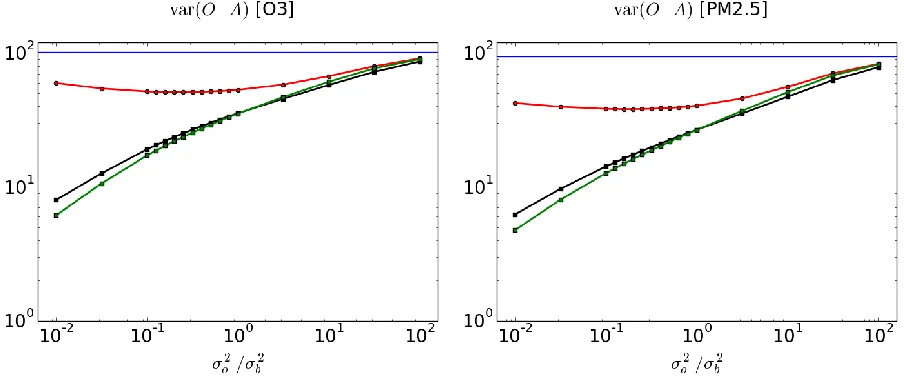
Figure 2. Variance of observation-minus-analysis residuals of O3 and PM2.5 for both active and
256
cross-validation passive observations as a function of
o2/
b2. Left panel is for O3 with257
ordinates in ppbv2 units, and right panel is for PM2.5 with ordinates in (
g/m3)2. Red curve258
results from the evaluation at the passive observation sites (average of the 3-fold subsets). Black
259
curves results from evaluation at the active observation sites with analyses using all
260
observations. Green curves results from the evaluation at the active observation sites in the
261
cross-validation experiment (i.e. using 2/3 of the observations; average of the 3 subsets). Blue
262
curve is the variance of observation-minus-model.
263
264
The var(OA) using passive observations (red curve with circles) and active observations (black
265
curve with squares) is presented in Figure 2 for O3 (left panel) and PM2.5 (right panel). The solid blue
266
line represents var(OB), the variance of observation-minus-model, i.e. prior to an analysis. As
267
mentioned in §2.4, in the cross-validation experiments we averaged the verification metric over the
3-268
fold subsets so that, in effect, the total number of observations that ends up being used for verification is
269
s
N , the total number of stations. We thus argue that the verification sampling error for the
cross-270
validation experiments (red curve) is the same as for the active observations using the full analysis (i.e.
271
analysis using the total number of stations; black curve). Also there is roughly 1,300 quality controlled
272
O3 observations over the domain and 750 PM2.5 quality controlled observations, each with 60 time
273
samples or less. To give some qualitative idea of the sampling error, the different metric values for the
274
individual 3-fold sets are presented in the supplementary material section, where we can see that for
275
)
var(OA and cor(O,A)the metric values for the individual sets are nearly indistinguishable from the
276
means of the 3-subset.
277
The difference between the verification against passive observations in cross-validation analyses
278
(red curve) and the verification against active observations using full analyses (black curve) can be
279
attributed to two effects: 1- the analysis used in the cross-validation uses 2/3rd of the total number of
280
observations and thus the analysis error has larger variance than analyses using all observations, 2- there
281
is a distance effect between the passive observation sites and the active ones for the analyses using 2/3rd
282
of the observations. In order to separate these two effects, we also display the 3-fold average of the
283
metric verifying against active observation for the cross-validation analyses as a green curve with
284
• red curve : using analysis with 2Ns/3 observations with an evaluation at passive sites
286
• green curve: using analysis with 2Ns/3 observations with an evaluation at active sites
287
• black curve : using analysis with Ns observations with an evaluation at active sites.
288
The difference between the red and green curves show the influence of distance between passive and
289
active observation sites, whereas the difference between the green and black curves show the influence
290
of having different number of observations in creating the analysis for verification.
291
Now let us examine the results of verifying against passive observations with cross-validation
292
analyses. As the observation weights gets smaller (i.e.
1), the analysis draws closer to the293
background, so that var(OA) increases toward var(OB). On the other end when
1,the294
analysis tries to overfit active observations which results in a spatially noisy analysis, which explains that
295
)
var(OA increases as
diminishes. Somewhere in between lies a minimum of var(OA) where296
there is neither an overfitting nor an underfitting to the active observations. This “optimal” ratio
297
actually corresponds the optimal analysis as we shall discuss in Part II of this study.
298
Now examining the results of verifying against active observations gives a different message. The
299
verification against active observations is presented with the black curves for the full analyses and with
300
the green curves for the cross-validation sets; the difference between the two curves being the number of
301
observations used to generate the analyses. In both curves we observe that var(OA) is steadily
302
decreasing as the observation weigth increases. In effect, it is an expected result from the inner working
303
of an analysis scheme that the analysis error variance does not depend on the observed values or the
304
model values. For this reason, the var(OA) using active observations cannot provide a true measure
305
of the quality of an analysis. There is, however, an exception to this when the analysis is optimal as we
306
shall see in Part II of this paper.
307
One would expect from having a larger number of observations in the analysis that the var(OA)
308
for the cross-validation analyses be slightly smaller than the var(OA) for the full analysis. This is
309
observed between the black and green curves when the observation weight is small (i.e.
1).310
However, and surprisingly when the observation weight is large,
1, we observe the opposite. This311
intriguing behavior may indicate an inconsistency between the assumption of uniform error variances
312
for
o2 and
b2 (assumed in the input error statistics) and the real spatial distribution of error variances.313
This discrepancy being simply amplified when the observation weight is large and when there are less
314
observations to produce the analysis.
315
The difference between var(OA) at passive sites and active sites (with the same number of
316
observations to construct the analyses) is significant. For O3 and for an optimal ratio, the var(OA) at
317
passive sites is 51.02 ppbv2 (red curve) while at active sites is 22.77 ppbv2 (green curve). For PM2.5 and
318
for an optimal ratio, the var(OA) at passive sites is 38.09 (
g/m3)2(red curve) while at active sites is319
15.41 (
g/m3)2(green curve). For both species, the error variance at active sites gives a significant320
overestimation of the error variance by more than a factor 2.
321
In Figure 3, we present the correlation metric between the observations and the analysis using, as in
322
Figure 2, the verification against passive observations in cross-validation analyses (red curve), the
323
verification against active observations using full analyses (black curve) and the verification against
324
active observations in the cross-validation analyses (green curve). The blue curve depict the correlation
325
between the model and the observations, that is the prior correlation.
326
328
Figure 3. Correlation between observations and analysis for O3 and PM2.5 for both active and
329
cross-validation passive observations as a function of
o2/
b2. The red, black and green330
curves are as in Figure 2.
331
332
The evaluation against passive observations with cross-validation analyses (red curve) shows a
333
maximum at the same values of
o2/
b2 than for the var(OA) . We argue that the same334
arguments of underfitting and overfitting are responsible for this maximum. The correlation between
335
the active observations and the analysis (black and green curves) increases as the observation weight
336
increases (
decreases), theoretically reaching a value 1 for
o2 0, which is again unrealistic and337
simply shows the impact of ill-prescribed error statistics in an analysis scheme. The gain in correlation
338
between independent observations and analysis is significant. For O3 , it increases from a value of 0.55
339
with respect to the model to a value of 0.74 with respect to an optimal analysis (when
o2/
b2 is340
optimal). For PM2.5 , the correlation against the model has a value of 0.3 which basically has no skill, to
341
a value of 0.54 for optimal analysis, which represent a modest but useable skill. The correlation
342
evaluated at the active sites for an optimal ratio, is 0.85 for O3 (green curve) and 0.74 for PM2.5 (green
343
curve), again being a significant overestimation with respect to values obtained at passive sites.
344
345
346
347
348
349
350
351
352
353
354
355
356
357
358
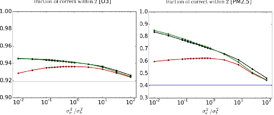
Figure 4. Fraction of correct within a factor 2 for O3 (left panel) and PM2.5 (right panel) for both
359
active and cross-validation passive observations as a function of
o2/
b2. The red, black360
Another metric that we have considered is the fraction of correct within a factor 2, eq. (5) [3]. The
362
evaluation of this metric against passive and active observations is presented in Figure 4 for O3 (left panel)
363
and PM2.5 (right panel). Note that the scale in the ordinate is quite different between the left and right
364
panels. Although the results bear similarity with the correlation between O and A presented in Figure
365
3, the maximum with passive observations is reached at larger
values than those obtained for366
)
var(OA or cor(O,A), which are identical. One possible explanation is that biases in observations and
367
analysis are not removed in the metric which could explain the shift of the maximum.
368
The interpretation of this metric is, however, not clear. Although the ratio zA/O is a
369
dimensionless quantity the spread of z is generally not independent of the variance of A or O and there
370
are cases where it is. So to count the number of occurrence of z between the dimensionless values 0.5
371
and 2 is confusing. As a simplified illustration, suppose that A is normally distributed as N(0,
a2) and372
similarly with O~N(0,
o2). The ratio of these two random variables is then a Cauchy distribution373
whose probability density function (pdf) is
o
a/[
(
o2z2
a2)]. The mean, variance and higher374
moments of Cauchy probability distributions are not defined since the integral of the pdf is not bounded;
375
only the mode is defined. Cauchy distributions also have a spread parameter, which in this case is equal
376
to
a/
o. If the variance of A and O are equal, then the number count between the dimensionless377
bounds 0.5 and 2 depends only on the shape of the probability distribution function, not on the variance.
378
If the variance of A and O are different, then it also depends on the ratio of variances. Furthermore, this
379
metric also depends on the bias. It is a difficult metric to interpret and overall it is unclear what new
380
information it adds. If used as a quality control, however, the FC2 have the unique ability of rejecting
381
too low as well as too high values of z.
382
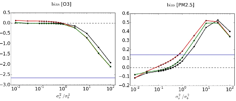
In Figure 5 we present the bias between observations and analyses, and were the verification is made
383
against passive and active observations as done with the other metrics. Bias is not a dimensionless
384
quantity; note that the range and scale presented for O3 and PM 2.5 in Figure 5 are different. The blue
385
curve is the mean (OB) and thus indicates for O3 in average over all observation stations (for the time
386
and dates considered) the model overpredicts, and that for PM2.5 the model underpredicts.
387
388
389
390
391
392
393
394
395
396
397
398
399
400
401
Figure 5. Bias between observation and analysis for O3 (left panel) and PM2.5 (right panel) for
402
both active and cross-validation passive observations as a function of
o2/
b2. The red,403
black and green curves are as in Figure 2.
404
Contrary to all metric results seen so far, the sampling uncertainty of the bias is significant: it is of
405
the order of 0.5 ppbv (in average) for O3 at passive sites and of the order of 0.1
g /m3 (in average)406
for the PM2.5 at passive sites (results shown in the supplementary material). The distinction between the
407
analysis bias and model bias is nearly always significant. For O3 , the model bias is eliminated at the
409
passive observation sites (red curve) as long as the observation weight
1. The situation is not so410
clear for PM2.5. In fact, when the observation weight is small, the bias result indicates that the analysis
411
has a larger bias than the model. How can that be when the observation weight is small (i.e.
1) and412
thus the analysis should be close to the model values? This apparent contradiction reveals a more
413
complex issue underlying the bias metric.
414
To explore the possible causes, we have calculated the bias per bin of model values, displayed in
415
Figure 6.
416
A)
417
418
419
420
421
422
423
424
425
426
427
428
429
430
431
B)
432
433
434
435
436
437
438
439
440
441
442
443
444
445
446
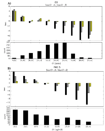
Figure 6. Biases per bin of model values. In A), presents the statistics for O3 and in B), for PM2.5.
447
In the upper portion of figures A) and B) are the residual statistics per bin; in black, the (OB)
448
, in grey, the (OA) at passive observation sites (mean of the 3-fold subsets) for a non-optimal
449
analysis with
10, and in yellow, the (OA) at passive observation sites (mean of the3-450
fold subsets) using the optimal observation weight. The lower portion of the figures A) and B)
451
are the station number count per model values.
452
453
In order have decent sample size per bin, we collect all the (OA) and (OB) over time and
454
before). The result shows that the model bias is nearly linearly dependent on the model (black boxes in
456
the bias panel). Both O3 and PM2.5 show an underprediction for low model values and an overprediction
457
for large model values. The origin of this bias is not known but one would argue that it is not related to
458
chemistry since both constituents, O3 and PM2.5, present the same feature. In the lower panels of A) and
459
B) shows the count of stations per model bin size. We observe that the majority of stations have O3
460
model values in the range of 40 to 55 ppbv, where the bias is negative. Over all the stations, this give
461
rise to a negative mean (OB), and this is how we claim that claim that the model overpredicts.
462
However, for PM2.5 the situation is different: the majority of stations lie in the low model value range,
463
and there are gradually less stations for increasingly larger model values. Although the (OB) have
464
large negative values in the high model value bin while small model value bins have positives (OB)
465
’s, the effect over all stations is to yield a modestly positive mean (OB) and thus the model
466
underestimates the PM2.5. The results of the analysis evaluated at the passive observation sites are
467
presented with the yellow and grey histogram boxes. In yellow, near optimal analyses with optimal
468
observation weight, as determined by the minimum of var(OA) are used, and in grey non-optimal
469
analyses with
10. We observe that the effect of the optimal analysis is nearly insentive to model bin470
values, where near zero biases are obtained in most of the range except for very small and very large
471
model values. The fact that we are not able to capture the full benefit of analysis on all model values
472
may be an artefact of the assumption that we are using uniform observation and background error
473
variances whereas the model values varies considerably. In grey, we used the non-optimal analyses
474
with a small observation weight were we set
10. In the non-optimal case, the state-dependent bias475
is still present but appears to be nearly perfectly anti-symmetric, positive in the low model value bins
476
and nearly exact opposite in high model value bins. Since for O3 the majority of observations lies in the
477
range 40 to 55 ppbv, (OA) for the optimal analyses at passive observation sites is nearly zero. But,
478
for the non-optimal analysis with
10, the (OA) at passive sites is negative, i.e. the analysis is479
overpredicting, as shown in Figure 5.
480
481
482
483
484
485
486
487
488
489
490
491
492
493
494
495
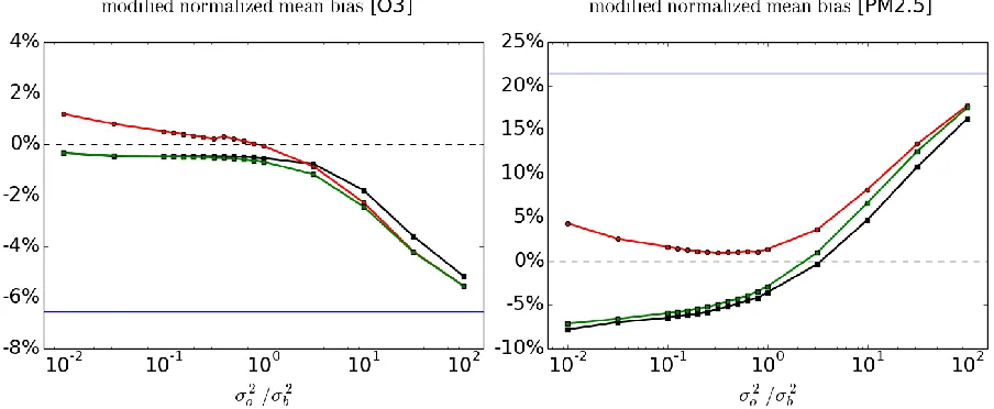
Figure 7. Modified normalized mean bias (MNMB) between observation and analysis for O3
496
(left panel) and PM2.5 (right panel) for both active and cross-validation passive observations as
497
a function of
o2/
b2. The red, black and green curves are as in Figure 2.498
499
For PM2.5 , the weighted sum of the (OA) bins is such that over all stations the bias for an optimal
500
nearly anti-symmetric (OA) bias per bin gives more weight to the positive bias at smaller model
502
values, so that overall there is a positive (OA), as in Figure 5.
503
To circumvent the state-dependency of the (OA) biases it is useful to consider instead a fractional
504
bias metric, such as the modified normalized mean bias, MNMB eq.(4). The MNMB metric is a
505
dimensionless measure and as defined with a factor 2, eq.(4), represents a % error. The MNMB for O3
506
and PM2.5 for passive and active observations are displayed in Figure 7 using the same color as in Figure
507
2. We note immediately that the MNMB analysis bias does not exceed the MNMB model bias as we
508
observed for the bias metric of PM2.5 (Figure 5 right panel). The MNMB bias also varies smoothly as a
509
function of
(at variance with the bias metric for PM2.5 – Figure 5).510
A)
511
512
513
514
515
516
517
518
519
520
521
522
523
524
525
B)
526
527
528
529
530
531
532
533
534
535
536
537
538
539
540
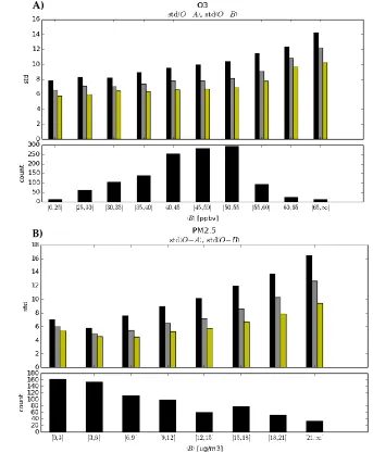
Figure 8. Same as Figure 6 except that we display the variance of analysis-minus-passive
541
observations per bin of model values.
542
543
Furthermore the sampling uncertainty of the analysis MNMB relative to the model bias (see the
544
supplementary material) is smaller than the relative uncertainty of the analysis bias with respect to the
545
model bias. This is especially true for PM2.5, where we can actually deduce that the difference between
546
the cross-validation and the validation against active observations is significant when
1. There is547
thus so happens that for a near optimal analysis the fractional bias MNMB is very small, around 1% for
549
O3 and about 1-2% for PM2.5. We argue that it results from an optimal use of observations.
550
There is also some information to gain from the variance of observed-minus-analysis per bin size,
551
as illustrated in Figure 8, using the same color histograms as in Figure 6. We note that for O3, the model
552
error variance against observations increases gradually with larger model values. But the fraction of
553
analysis variance vs. model variance is roughly uniform across all bins. This can be explained by the
554
fact that the observation and background error variances are uniform, and thus the reduction of variance
555
across all bins is uniform as well. However, the situation is different for PM2.5. We note a relatively
556
poor performance of the model at low model values, with standard deviation of 7g/m3. For slightly
557
larger model values (3-6 g/m3), the error variance is smaller to 5.5g/m3 and then increases almost
558
linearly with model values. The fraction of analysis variance vs. model variance decreases steadily with
559
larger model values. These results thus indicate that the assumption that observation and background
560
error variances are uniform and independent of the model value may have to be revisited.
561
4. Conclusions
562
We have developed an approach by which analyses can be evaluated and optimized without using
563
a model forecast but rather by partitioning the original observation data set into a training set, to create
564
the analysis, and an independent (or passive) set, used to evaluate the analysis. This kind of evaluation
565
by partitioning is called cross-validation.
566
The need for such a technique came about our desire to evaluate our operational surface air quality
567
analyses that are created off-line with no assimilation cycling. Evaluating a surface air quality analysis
568
based on its chemical forecast does in fact require additional information or assumptions, such as vertical
569
correlation, aerosol speciation and bin distribution (while surface measurement is primarily about mass)
570
or unobserved chemical variables correlations, and so on…. So that the quality of the chemical forecast
571
is not solely dependent on the quality of the analysis and, if there are compensating errors, can actually
572
be a misleading assessment of the quality of the analysis.
573
We have applied this cross-validation procedure to the operational analyses of surface O3 and PM2.5
574
over North America for a period of 60 days and present an evaluation using different metrics; bias,
575
modified normalized mean bias, variance of observation-minus-analysis residuals, correlation between
576
observation and analysis, and fraction of correction within a factor 2.
577
Our results show that, in terms of variance and correlation, the verification of analyses against active
578
observations always yield an overestimation of the accuracy of the analysis. This overestimation also
579
increases as the observation weight increases. On the other hand for biases, the distinction between the
580
verification against active observations and passive observations is unclear and drowned in the sample
581
variability. However, using a fractional bias metric, in particular the MNMB, shows that the verification
582
against passive observations can be close to one percent for an optimal analysis while the verification
583
against active observations is much larger.
584
Results also show the importance of having an optimal analysis for verification. The variance of
585
the analysis with respect to independent observations is minimum and the correlation between the
586
analysis and independent observations is maximum for an optimal analysis. By being a compromise
587
between an overfit to the active observations (which produce noisy analysis field) and an underfit, the
588
optimal analysis offers the best use of observations throughout. At optimality, the analysis fractional
589
bias (MNMB) at the passive observation sites has only one or two percent error whereas the fractional
590
bias of the model is 6.5% for O3 and 21% for PM2.5. The correlation between the analysis and
591
independent observations is also significantly improved with an optimal analysis: the correlation
592
between the model and independent observations is 0.55 for O3 and increases to 0.74 with the analysis,
593
while for PM2.5 the correlation between the model and independent observations is only 0.3 (which is
594
We also argue that the fraction of correct within a factor 2, is a metric whose interpretation is unclear
596
as it mixes information about bias, variance and probability distribution in a non-uniform way and does
597
not seem to add anything new to other metrics. The bias is also very sensitive to sample variability and
598
can lead to wrong conclusions. For example, we have seen that the mean analysis bias can be larger
599
than the mean model bias, whether verifying against active or passive observations. But, since an analysis
600
is always closer to the truth than its prior (i.e. the model), it results in an apparent contradiction. This
601
implies that the bias metric cannot be used to faithfully compare model states accurately. Such wrongful
602
conclusions do not arise, however, with the MNMB. We thus recommend avoiding using bias as a
603
measure of truthfulness, and use instead a fractional bias measure such as the MNMB.
604
We also found that errors in the GEM-MACH model grow almost linearly with the model value.
605
This is particularly evident for the bias where the model underestimates at small model values and
606
overestimates at large model values. Furthermore this occurs in equal ways for O3 and PM2.5, thus
607
indicating that the source of this bias is not related to chemistry. The fact that, over the entire domain,
608
the model overestimates O3, and underestimates PM2.5 is simply a result of the concentrations. We have
609
not conducted a systematic study of model error for other times of the day and other periods of the year,
610
but it would be very interesting to look at this, to see whether or not changes of biases are due primarily
611
to changes in the distribution of values rather than a fundamental change in the bias per model value
612
bin.
613
Finally we have also examined the variance against independent observations per model value bin
614
, and concluded that the error variance is not quite uniform with model values but increases slowly with
615
model values for O3 and in a more pronounced way for PM2.5.
616
In Part II, we will focus on the estimation of the analysis error variance and develop a mathematical
617
formalism that permits to compare different diagnostics of variance under different assumptions,
618
optimize the analysis parameters and gain confidence on the estimate of analysis error as we obtain
619
coherent estimated values across different diagnostics.
620
621
Supplementary Materials: The following are available online at www.mdpi.com/link, Figure S1: Verification of
622
variance for O3 and PM2.5 for the individual sets. Figure S2: Same as Figure S1 but for the correlation between
623
observations and analysis. Figure S3: Same as Figure S1 but for the fraction of correct within a factor 2. . Figure S4:
624
Same as Figure S1 but for bias. . Figure S5: Same as Figure S1 but for modified normalized mean bias.
625
Acknowledgments: We are grateful to the US/EPA for the use of the AIRNow database for surface pollutants and
626
to all provincial governments and territories of Canada for kindly transmitting their data to the Canadian
627
Meteorological Centre to produce the surface analysis of atmospheric pollutants. We are also thankful for the proof
628
read by Kerill Semeniuk, and for two anonymous reviewers for their comments and help in improving the
629
manuscript.
630
Author Contributions: This research was conducted as a joint effort by both authors. R.M. contributed to the
631
theoretical development and wrote the paper, and M.D.-J. conducted all experiments design and execution, proof
632
reading and introduced a new diagnostic of optimal analysis error that was furher extended to passive observations
633
space.
634
Conflicts of Interest: The authors declare no conflict of interest. The founding sponsors, which is the government
635
of Canada, had no role in the design of the study; in the collection, analyses, or interpretation of data; in the writing
636
of the manuscript, and in the decision to publish the results.
637
638
References
639
1. Ménard, R., and A. Robichaud. The chemistry-forecast system at the Meteorological Service of Canada. In
640
2. Robichaud, A. and R. Ménard. Multi-year objective analysis of warm season ground-level ozone and PM2.5
642
over North-America using real-time observations and Canadian operational air quality models. Atmos. Chem.
643
Phys. 2014. 14:1769-1800. DOI: 10.5194/acp-14-1769-2014.
644
3. Robichaud, A., R. Ménard, Y. Zaïtseva, and D. Anselmo. Multi-pollutant surface objective analyses and
645
mapping of air quality health index over North America. Air Qual. Atmos. Health. 2016, DOI
10.1007/s11869-646
015-0385-9.
647
4. Moran, M.D., S. Ménard, R. Pavlovic, D. Anselmo, S. Antonopoulus, A. Robichaud, S. Gravel, P.A. Makar, W.
648
Gong, C. Stroud, J. Zhang, Q. Zheng, H. Landry, P.A. Beaulieu, S. Gilbert, J. Chen, and A. Kallaur. Recent
649
advances in Canada’s national operational air quality forecasting system. 32nd NATO-SPS ITM, Utrecht, NL,
650
7-11 May 2012.
651
5. Pudykiewicz, J.A., A. Kallaur, and P.K. Smolarkiewcz. Semi-lagrangian modelling of tropospheric ozone.
652
Tellus, 49B, 1997, 231-248.
653
6. Carmichael, G.R., A. Sandu, T. Chai, D.N. Daescu, E.M. Constantinescu and Y. Tang. Predicting air quality :
654
Improvements through advanced methods to integrate models and measurements. J. Comput. Phys., 227, 2008,
655
3540-3571.
656
7. W.F. Dabberdt, M.A. Carroll, D. Baumgardner, G. Carmichael, R. Cohen, T. Dye, J. Ellis, G. Grell, S. Grimmond,
657
S. Hanna, J. Irwin, B. Lamb, S. Madronich, J. McQueen, J. Meagher, T. Odman, J. Pleim, H.P. Schmid, D.L.
658
Westphal, Meteorological research needs for improved air quality forecasting – Report of the 11th prospectus
659
development team of the US weather research program, Bull. Amer. Meteorol. Soc. 85 (4), 2004, 563.
660
8. Sportisse, B.. A review of current issues in air pollution modeling and simulation. Comput. Geosci., 2007,
11:159-661
181. DOI 10.1007/s10596-006-9036-4.
662
9. Elbern, H., A. Strunk, and L. Nieradzik. Inverse modelling and combined state-source estimation for chemical
663
weather. In Data Assimilation: Making Sense of Observation (eds. Lahoz, W, B. Khattatov, and R. Ménard),
664
Springer, 2010, 491-513.
665
10. Bocquet, M., H. Elbern, H. Eskes, M. Hirtl, R. Žabkar, G.R. Carmicheal, J. Flemming, A. Inness, M. Pagaoski,
666
J.L. Pérez Camaño, P.E. Saide, R. San Jose, M. Sofiev, J. Vira, A. Baklanov, C. Carnevale, G. Grell, and C.
667
Seigneur. Data assimilation in atmospheric chemistry models; current status and future prospects for coupled
668
chemistry meteorology models. Atmos. Chem. Phys., 15, 5325-5358, 2015,
www.atmos-chem-phys-669
net/15/5325/2015/, doi: 10.5194/acp-15-5325-2015.
670
11. T. Chai, G.R. Carmichael, A. Sandu, Y.H. Tang, D.N. Daescu, Chemical data assimilation of transport and
671
chemical evolution over the pacific (TRACE-P) aircraft measurements, J. Geophys. Res. 111 (D02301), 2006,
672
doi:10.1029/2005JD005883.
673
12. Sandu, A., and T. Chai. Chemical data assimilation–An overview. Atmosphere 2011, 2, 426-463;
674
doi:10.3390/atmos2030426.
675
13. Marseille, G.-J., J. Barkmeijer, S. de Haan, and W. Verkley. Assessment and tuning of data assimilation systems
676
using passive observations. Q. J. R. Meteorol. Soc., 2016, 142, 3001-3014, DOI:10.1002/qj.2882.
677
14. Ménard, R., M. Deshaies-Jacques, and N. Gasset. A comparison of correlation-length estimation methods for
678
the objective analysis of surface pollutants at Environment and Climate Change Canada. Journal of the Air &
679
Waste Management Association. 2016, 66:9, 874-895, DOI: 10.1080/10962247.2016.1177620.
680
15. Cohn, S.E., A. da Silva, J. Guo, M. Sienkiewicz, and D. Lamich. Assessing the effects of data selection with the
681
DAO physical-space statistical analysis system. Mon. Wea. Rev. 1998, 126, 2913–2926.
682
16. Houtekamer, P.L., and H.L. Mitchell. A sequential ensemble Kalman filter for atmospheric data assimilation.
683
Mon. Wea. Rev. 2001, 129,123-137.
684
17. Efron, B. An introduction to boostrap. Chapman & Hall: New York, 1993, 436 pp.
685
18. Seigneur, C., B. Pun, P. Pai, J.-F. Louis, P. Solomon, C. Emery, R. Morris, M. Zahniser, D. Worsnop. P. Koutrakis,
686
W. White and I. Tombach. Guidance for the performance evaluation of three-dimensional air quality modeling
687
systems for particulate matter and visibility. Journal of the Air & Waste Management Association. 2000, 50:4,
688
588-599, DOI: 10.1080/10473289.2000.10464036 .
689
19. Chang, J.C. and S.R. Hanna. Air quality model performance evaluation. Meteorol. Atmos. Phys.. 2004, 87,
167-690
20. Savage, N.H., P. Agnew, L.S. Davis, C. Ordóñez, R. Thorpe, C.E. Johnson, F.M. O’Connor, and M. Dalvi. Air
692
quality modelling using the Met Office Unified Model (AQUM OS24-26): model description and initial
693
evaluation. Geosci. Model Dev.. 2013, 6, 353-372, www.geosci-model-dev.net/6/353/2013/
694
21. Katragkou, E., P. Zanis, A. Tsikerdekis, J. Kapsomenakis, D. Melas, H. Eskes, J. Flemming, V. Huijnen, A. Inness,
695
M.G. Schultz, O. Stein, and C.S. Zerefos. Evaluation of near surface ozone over Europe from the MACC
696
reanalysis. Geosci. Model Dev. 2015, 8, 2299-2314, https://doi.org/10.5194/gmd-8-2299-2015
697
22. Ménard, R. Error covariance estimation methods based on analysis residuals: theoretical foundation and
698
convergence properties derived from simplified observation networks. Q. J. R. Meteorol. Soc.. 2016, 142,
257-699
273, DOI:10.1002/qj.2650.
700
23. Desroziers, G., L. Berre, B. Chapnik, and P. Poli. Diagnosis of observation-, background-, and analysis-error
701
statistics in observation space. Q. J. Roy. Meteorol. Soc. 2005, 131, 3385-3396.
702