Realistic FDTD GPR antenna models optimized using a novel linear/non-linear full waveform inversion

Realistic FDTD GPR antenna models optimised

using a novel linear/non-linear Full Waveform

Inversion

Iraklis Giannakis, Antonios Giannopoulos, and Craig Warren

Abstract—Finite-Difference Time-Domain (FDTD) modelling of Ground Penetrating Radar (GPR) is becoming regularly used in model-based interpretation methods like full waveform inversion (FWI), and machine learning schemes using synthetic training data. Oversimplifications in such forward models can compromise the accuracy and realism with which real GPR responses can be simulated, and this degrades the overall performance of the aforementioned interpretation techniques. Therefore, a forward model must be able to accurately simulate every part of the GPR problem that can affect the resulting scattered field. A key element is the antenna system and excitation waveform, so the model must contain a complete description of the antenna including the excitation source and waveform, the geometry, and the dielectric properties of materials in the antenna. The challenge is that some of these parameters are not known or easily measured, especially for commercial GPR antennas that are used in practice. We present a novel hybrid linear/non-linear FWI approach which can be used, with only knowledge of the basic antenna geometry, to simultaneously optimise the dielectric properties and excitation waveform of the antenna, and minimise the error between real and synthetic data. The accuracy and stability of our proposed methodology is demonstrated by successfully modelling a Geophysical Survey Systems (GSSI) Inc. 1.5 GHz commercial antenna. Our framework allows accurate models of GPR antennas to be developed without requiring detailed knowledge of every component in the antenna. This is significant because it allows commercial GPR antennas, regularly used in GPR surveys, to be more readily simulated.

Keywords—Antennas, commercial, FDTD, FWI, GPR, hybrid optimisation, linear inversion, non-linear inversion.

I. INTRODUCTION

Ground Penetrating Radar (GPR) has been successfully applied to sensing problems across a wide spectrum of scales – from landmine detection at very shallow depths, to mapping the thickness of glaciers [1]. Consequently, different antennas have been proposed in order to address the unique require-ments of each GPR sensing problem – dipoles [2], bowties [3], horns [4], spirals [5], and more complicated non-conventional antennas [6] specifically designed for GPR applications using different sizes, excitation pulses, and absorbing materials [1]. Despite the diversity of real GPR antennas, numerical models

I. Giannakis and A.Giannopoulos are with the School of Engineer-ing, The University of Edinburgh, Edinburgh, EH9 3FG, UK. E-mail: [email protected] and [email protected]

C. Warren is with the Department of Mechanical and Construction Engineering, Northumbria University, Newcastle, NE1 8ST, UK. E-mail: [email protected] .

often include basic excitation models and simplified antenna structures [7], [8], [9] which can lead to generic and non-exact outputs when these models are used to compare real to predicted GPR data.

The antenna system is a dominant part of the simulation and should be accurately modelled if the simulation is to replicate the behaviour of a given GPR system [10], [11]. The directivity pattern, ringing noise, shape of the waveform, and the coupling between the antenna and the ground are directly related to the antenna system [10], [12]. Models using simplified excitation sources, such as Hertzian dipoles, especially for high frequency applications, can produce significantly different responses from real measurements [10]. Therefore, these models cannot be easily employed either as a forward solver for inversion purposes, or for generating synthetic training sets for machine learning applications [13].

IEEE TRANSACTIONS ON GEOSCIENCE AND REMOTE SENSING 2 simulations and the need for accurate knowledge of the antenna

geometry, dielectric properties etc... The main drawbacks of this approach are that it requires knowledge of the system excitation, and it assumes that the scattering sources are placed in the far-field region of the antenna [4]. Hence, equivalent sources were successfully applied primarily for modelling custom made off-ground horn antennas [4], [23], [24]. In [25], an equivalent sources scheme is suggested which models the global reflection and transmission coefficients in an effort to model the near-field behaviour of a custom made Vivaldi antenna. The near-field formulation has been successfully tested in layered media, but further validation is needed in more realistic scenarios.

As computational resources have increased in power and accessibility, numerical modelling of antennas using FDTD gained in popularity [26]-[33]. Nonetheless, commercial an-tennas, which are available to the end-user, remained a black box and only a few researchers have tried to tackle this issue by fully simulating a commercial GPR system [10], [34], [35]. In [10] and [34], a 1.5 GHz commercial antenna from Geophysical Survey Systems (GSSI) Inc. is modelled using FDTD. A fine 1 mm grid is employed in an effort to minimise numerical dispersion [15] and avoid staircasing effects. Furthermore, a Taguchi optimisation is used in order to fine-tune the dielectric properties of the antenna. The cost function of the optimisation is the difference between the real and the synthetic free-space response. A Gaussian voltage source is used as an excitation, and the central frequency is decided from the Taguchi optimisation. This limits the accuracy of the resulting antenna model since it constrains the pulse to be Gaussian-shaped. Using global optimisers to derive the optimised pulse without any given constraints will vastly increase the optimisation parameters which will, in turn, increase the required computational resources to an unreasonable level.

In this paper, in order to address this issue, instead of a Taguchi optimisation, a hybrid linear/non-linear least squares scheme that simultaneously updates the dielectric properties and the corresponding optimised pulse is introduced. We use a non-linear least squares optimisation to fine-tune the dielectric properties of a given antenna and simultaneously the optimised pulse is expressed linearly with respect to these properties. Thus, the shape of the pulse is not bounded by any constraints, and the computational requirements of the optimisation are not increased.

A similar hybrid linear/non-linear optimisation is proposed in [36] to evaluate the optimised wavenumbers for solving the 2.5-D Helmholtz equation for electrical resistivity tomography. A modified version of [36] using particle swarm optimisation is suggested in [37] in order to approximate Havriliak-Negami functions with multi-Debye expansions. The simultaneous evaluation of the medium parameters and of the effective wavelet in seismic FWI has been a subject of investigation since the early 1980’s [38], [39]. For GPR, wavelet estimation as part of FWI has been successfully applied by different authors mostly for cross-borehole applications. In particular, a hybrid least-squares/simplex-search FWI is employed in [40], assuming a homogeneous half space and using a single dipole

to describe the antenna system. In [41] and [42] a FWI scheme is proposed in which the pulse is part of the unknowns and the applicability of multiple wavelets is examined to address the fact that the effective wavelet is affected by the location of the transmitter. This results from describing the antenna with a single point source without incorporating its physical structure in the numerical model. A similar approach is used by [43] to tackle the challenging problem of estimating the radius of a rebar inside concrete. In [44], a hybrid least-squares/cascaded algorithm is used in order to approximate a Wu-King type antenna by equivalent sources. The resulting antenna approximates the far field behaviour of the actual antenna with sufficient accuracy. Similar to all the approaches that employ equivalent sources, the modelled antenna in [44] does not contain any information regarding the near-field interactions of the antenna structure with the background, thus it is not recommended for modelling ground-coupled antennas especially for high frequency near-field problems. Lastly, effective wavelet estimation of point sources prior to FWI is also applied by [45] for cross-borehole tomography, and [46] for estimating the chloride content of concrete.

Apart from [36], all the papers mentioned above that use gradient-based optimisation approaches, do not include the linear part of the inversion in the evaluation of the partial derivatives. In other words, the gradients are calculated given that the output of the linear part, the effective wavelet, is constant in each step and is not affected by the variation of the non-linear parameters related to the medium properties. In this paper we follow the approach in [36], but instead of using a central-difference method we evaluate the Jacobian analyt-ically. As far as we are aware, such an analytical evaluation of the true Jacobian in hybrid linear/non-linear optimisation problems has not been attempted before.

To avoid instabilities in the linear step of the optimisation, in contrast to [40] and [44], a Levenberg-Marquardt damped least squares method [47], also known as Tikhonov regularization method [48], [49]) is used, and all the calculations take place directly in time domain. A similar regularisation method is applied in the frequency domain in [46] to evaluate an effective wavelet prior to FWI. Nonetheless, the regularisation parameter in [46] is chosen in an arbitrary manner and the authors do not address the sensitivity of the deconvolved pulse to the regularisation parameter. Here, the regularisation parameter is chosen based on the L-curve method [50], [51] which balances accuracy and stability.

the Jacobian matrix for hybrid linear/non-linear inversion and the L-curve approach can be extrapolated in a similar manner for traditional GPR and seismic FWI for which the effective wavelet is part of the unknown parameters.

II. HYBRIDLINEAR/NON-LINEARINVERSION

The proposed inversion scheme is intended to be applied to antennas with unknown dielectric properties and excitation sources. This is a common occurrence when modelling com-mercial antennas for which these properties are unknown for confidentiality reasons. Nonetheless, the geometrical properties of the antenna can usually be obtained by inspection. Thus, in the proposed hybrid FWI it is assumed that the geometry of the antenna is known and accurately modelled in the FDTD numerical simulator.

Another assumption of the proposed FWI is linearity, which is valid for the majority of electromagnetic (EM) problems [15] when low amplitude fields are used. The linear step of the optimisation is a constrained deconvolution. Consequently, non-linear EM phenomena are assumed to be negligible, and dielectric properties are not related to the amplitude of the field. In addition, the FDTD forward solver used in this paper implements linear isotropic media. Using a forward solver that incorporates non-linear media would greatly increase the complexity and computational resources of every aspect of the FWI.

The modelled antenna is not necessarily an exact replica of the real antenna. It is an apparent antenna that is intended to accurately replicate the behaviour and per-formance of the real antenna.

A. Linear Least-Squares Inversion

The explicit representation of the received electric field due to a distribution of current densities is given by [52]

Es= Z

V Z τ

0

G(x,x0, t, t0)J(x0, t0)dt0dV (x0) (1) where, G= [Gx, Gy, Gz] is the Green’s function that acts on the current density vector J= [Jx, Jy, Jz],Es= [Ex, Ey, Ez] is the electric field,x0= [x, y, z]are the Cartesian coordinates of the transmitter, x are the Cartesian coordinates of the receiver,τ is time, andV is the investigated 3D volume.

For simplicity it is assumed that the transmitter and the receiver are at known positions and that the transmitter-receiver separation stays constant. This is a standard configuration for common-offset antennas most frequently employed in GPR applications [1]. In addition, the components of the excitation source and the received field are usually known and they are placed for convenience to be parallel to one of the Cartesian axes. Lastly, the unknown parts of the model are the dielectric properties of the antenna, thus, the Green’s function can be expressed with respect to the dielectric properties of the an-tenna assuming the rest of the model (i.e. chosen background) is constant throughout the FWI. Based on the above, equation (1) can be restated as

Es i =

Z τ 0

Gi,j(p, t, t0)Ij(t0)dt0 (2) where p = [p1, p2, p3...pn] is a vector that contains the dielectric properties of the antenna parts, assuming that the geometry is known, Ij is the induced current, j ∈ {x, y, z}

is the component of the transmitted field, andi_{∈ {}x, y, z_} is the component of the received field. For co-polarised antennas i=j.

Equation (2) is a convolution and can be re-written as Eis(p, t) =Gi,j(p, t)∗Ij(t) (3) Gi,j(p, t) =Gm,i,j(p, t)∗Gr,i,j(t) (4) Ij(t) =Pj(t)_∗Cj(t) (5) whereGi,j is expressed as the Green’s function of the model Gm,i,j convolved with the Green’s function of the receiver Gr,i,j. Notice that FDTD can model Gm,i,j using a delta function to excite the FDTD solver with sufficient accuracy for a specified frequency range. Nonetheless, electronic compo-nents in the antenna and post-processing associated withGr,i,j cannot be modelled using FDTD without prior knowledge. A similar division occurs in (5) in which the excitation source is expressed as a convolution between the initial applied pulse Pj (Gaussian, delta function and so on) with the correction Cj. As it is stated earlier, the above formulation is not valid when non-linear electromagnetic phenomena are present.

Due to the interchangeable nature of convolution, equation (3) can be written as

Esi(p, t) =Eic(p, t)∗Ri,j(t) (6) Eic(p, t) =Gm,i,j(p, t)∗Pj(t) (7) Ri,j(t) =Cj(t)_∗Gr,i,j(t). (8) Notice that Ec

i(p, t) can be evaluated for a given vectorp using FDTD excited byPj(t). The termRi,j(t)expresses the unknown receiver effects plus the correction that is convolved with the initial excitation source. The convolution in (6) can be numerically evaluated as follows

Q=KX (9)

K= 

      

Eic(p, t1) 0 . . . 0 Ec

i (p, t2) Eic(p, t1) . . . 0 Ec

i (p, t3) Eic(p, t2) . . . 0 Ec

i (p, t4) Eic(p, t3) . . . 0 ..

. ... . .. ...

Ec

i(p, tN) Eic(p, tN−1) . . . Eci(p, t1) 

      

IEEE TRANSACTIONS ON GEOSCIENCE AND REMOTE SENSING 4 that cannot be implemented in FDTD either due to a lack

of information or due to limitations of FDTD (e.g. modelling electronic components in the GPR transducer).

The idea behind the proposed method is to use a series of controlled experiments (e.g. direct coupling in free space) in order to fine tune an antenna model with a given geometry. The controlled measurements represent the Q vector, the measurements taken using the real antenna with the actual excitation pulse and the actual receiver effects. With a given geometry and a set of dielectric properties p, the matrix K can be calculated using FDTD. Subsequently the vector X is derived by solving the linear system of equations in (9).

Notice that when only one controlled experiment is used, the system of equations in (9) becomes well-determined and an exact fit will occur regardless of K, given det(K) 6= 0. Thus, approaches using only one controlled experiment [53] to calibrate the modelled antenna lead to non-uniqueness as the fitted function has higher dimensions compared to the data, similar to fitting the best line to a point. Hence, the resulting antenna is not reliable for universal applications despite the fact that the fit is good for the specific single controlled experiment. In addition, similar calibration approaches applied to either fre-quency or time domain need a regularisation parameter in order to overcome the instabilities arising from dividing by zero in frequency domain. This becomes clear when (6) is solved in the frequency domain Ri,jˆ (ω) = ˆEis(p, ω)/Eˆic(p, ω). Frequencies whereEˆc

i(p, ω)become close to zero are suscep-tible to noise and create instabilities that reduces the overall reliability of the resultingRi,j.ˆ

By using more than one controlled experiment the system of (9) becomes over-determined



     

Q₁ Q₂ . . . Q_M



     

= 

     

K1 K2 . . . KM



     

X (12)

where M is the number of controlled experiments. For convenience the following matrices are introduced

Y= [Q1,Q2, ...QM] T

(13) A= [K1,K2...KM]T. (14) The over-determined system can be solved using the Tikhonov regularised least-squares method

X=ATA+λ2I− 1

ATY (15)

where λis the regularisation parameter, and I is the identity matrix. The regularisation factor λ is added to suppress the resultingXvector and prevent its norm from reaching extreme values due to high signal-to-noise ratio at frequencies with amplitudes close to zero.

The X vector resulting from (15) minimises the following function min

X∈RN||

AX₋Y_||2₂+λ2

||X_||2₂ given a regularisation

parameter λ and a vector p, necessary to calculate A. The vectorp, and its corresponding optimisedX, that minimises the difference between the real and the synthetic measurements, is derived through the following non-linear optimisation.

B. Non-Linear Inversion

The dielectric properties of the antenna are assumed to be isotropic, linear, and dispersion-less. In other words, the dielectric properties of the different parts of the antenna are approximated with a constant permittivity and conductivity pb= [b, σb].

Substituting (15) to (12) results in Y=AATA+λ2I−

1

ATY. (16)

The only variables to be optimised in (16) are the dielectric properties of the antenna. The latter are given in vector form p= [p1, p2...pn], where nis the number of the antenna parts. The vector Xis now described algebraically as a function of A, i.e. as a function of the dielectric properties of the antenna. Thus, the dimensionality of the optimisation space is greatly reduced.

It is apparent that equation (16) is valid only when I=AATA+λ2I−

1

AT, (17)

which holds true regardless of p, if the system of equations (9) is well-determined using only one controlled experiment, for λ= 0, and when det(A)₆= 0.

When more than one controlled experiment is used, a non-linear least squares inversion is employed that minimises the following function

min

p∈Rn||

AATA+λ2I− 1

ATY₋Y_||2₂. (18) Introducing the vectorD

D=AATA+λ2I− 1

ATY, (19)

equation (18) can be simplified as min

p∈Rn||

D₋Y_||2₂. (20) Non-linear least squares inversion is an iterative method that linearises the problem in each iteration. An initial set of dielectric properties pis chosen which is used to evaluate the vector Dp. Subsequently, the vector Y is approximated by a

first-order Taylor series expansion

contains the partial derivatives of the vector Dwith respect to the dielectric properties p.

J= 

      

∂D1

∂p1

∂D1

∂p2

∂D1

∂p3 . . .

∂D1

∂pn

∂D2

∂p1

∂D2

∂p2

∂D2

∂p3 . . .

∂D2

∂pn

∂D3

∂p1

∂D3

∂p2

∂D3

∂p3 . . .

∂D3

∂pn

..

. ... ... . .. ... ∂DM·N

∂p1

∂DM·N

∂p2

∂DM·N

∂p3 . . .

∂DM·N

∂pn



      

Where ∂Dk

∂pg is a vector containing the partial derivatives with

respect to permittivity and conductivity ∂Dk

∂pg =

∂Dk ∂g ,

∂Dk ∂σg

. (20)

Using least squares the vector ∆pw in (21) is derived ∆pw=

JT_p

wJpw

−1 JT_p

w Y−Dpw

. (21)

Subsequently the vector p is updated

p_w+1=p_w+ ∆pw (22)

and the procedure is repeated until (18) converges to a minimum. Given an optimised set of dielectric properties p, the correction term X can be calculated in a straightforward manner using (15).

The hybrid linear/non-linear FWI evaluates permittivity and conductivity simultaneously in contrast to [54] in which a permittivity distribution is initially derived and subsequently the optimised conductivity profile is derived based on the pre-estimated permittivity distribution. This is due to the fact that [54] uses a gradient-based cascaded scheme in which the incremental step is defined by the user. This results in a bias towards permittivity changes since the sensitivity of conductivity is orders of magnitude less than the sensitivity of permittivity. A solution to this is given in [52] in which the incremental steps are adjusted accordingly in order to regulate the sensitivity discrepancies. The proposed FWI overcomes the aforementioned issues since the incremental step is calculated directly in (21). In the case study presented here, the pro-posed algorithm is proven to be stable and robust despite the sensitivity gap between permittivity and conductivity. In the presence of ill-conditioned Jacobians due to low sensitivity at parts of the antenna, inadequate controlled experiments etc., it is advised to use a Marquardt non-linear least squares [47].

Non-linear inversion is a convex optimisation and assumes that the initial model is relatively close to the real one. Convex optimisers are frequently employed in FWI for both GPR and seismic methods, and the importance of the initial model has been stressed by many authors [54], [55], [56]. The current method is proven to be not as sensitive to the initial conditions as a generic FWI. This is probably due to the fact that the geometry of the antenna is constrained and the unknown parameters are orders of magnitude smaller compared to 3D tomography. Nonetheless, it is preferable to choose a rational set for the initial vector p to ensure fast convergence and stability.

C. L-curve and selection of λ

Regularisation is an essential element in deconvolution in order to repress extreme solutions arising either from noise or from frequencies with amplitudes close to zero [1]. It is apparent that the final output of the deconvolution is sensitive toλselection and a systematic way of choosing an appropriate λshould be applied. Prior methods that neglect regularisation or chose it in an arbitrary manner result in unreliable outputs due to the non-uniqueness of the problem.

The well-known L-curve [50], [51] method is chosen in this paper in an effort to balance stability and accuracy. During the linear step of the FWI the following function is minimised

min

X∈RN||

AX₋Y_||2₂+λ2_||X||2

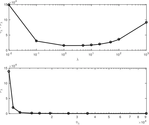
2 given a vector p, evaluated in the non-linear step, and λas defined by the user. The L-curve tries to balance the two parameters of the minimisation i.e. ηλ = _||AX₋Y_||2₂ and ρλ = _||X_||2₂. Large values of λ will repressρλwhile compromiseηλ. On the other hand, forλ= 0 the problem transforms to naive least-squares with small ηλ and unstable (large) ρλ.

Plotting (ηλ, ρλ)results in an exponentially decaying func-tion. A log-log plot of this function results in a curve that looks like the letter ‘L’, hence the name L-curve method. The λ value that corresponds to the critical point where ρλ starts to converge to a minimum is the point where min

λ∈R|| AX₋

Y_||2₂+_||X_||2₂given a vector p, and the controlled experiments Y. Here, a brute force approach is followed in which the hybrid linear/non-linear FWI is executed with different λ. Subsequently the L-curve is plotted and the appropriate λ associated with the critical point of the curve is chosen.

D. Jacobian calculation

The Jacobian matrix can be expressed in a more compact form as follows

J= _∂D

∂p1 ∂D ∂p2

. . . ∂D ∂pn

(23)

where

∂D ∂pg =

∂D1

∂pg ∂D2

∂pg . . .

∂DM·N ∂pg

T

. (24)

The simplest way to calculate the derivative is through a central finite-difference approximation (first order approximations can be applied in a similar manner)

∂D(pg) ∂pg ≈

D(pg+ ∆pg)−D(pg−∆pg)

2∆pg . (25)

From (19) and (24) it follows that the analytical expression of the Jacobian is

∂D ∂pg =

∂

AATA+λ2_I−1_AT

IEEE TRANSACTIONS ON GEOSCIENCE AND REMOTE SENSING 6

∂D

∂pg

= ∂A

∂pg

ATA+λ2I

−1

AT+A −ATA+λ2I

−1

∂A

∂pg T

A+AT∂A

∂pg !

ATA+λ2I

−1!

AT+AATA+λ2I

−1_∂AT

∂pg !

Y

(30)

Modelling commercial GPR antennas 3

cluster.

Another important aspect of creating models of GPR antennas is the ability to visualise, in 3D, their detailed ge-ometrical features. Modelling these features required set-ting the properties of faces and edges of Yee cells in a finely discretised FDTD grid. ParaView (http://www.paraview.org/) is an open-source data-analysis and visualisation

applica-tion based on the Visualisaapplica-tion Toolkit (VTK) (http://www.vtk.org/) and has been developed for handling extremely large datasets.

The VTK is an open-source system for 3D computer graph-ics, image processing and visualisation. The VTK uses Extensible Markup Language (XML) files to define struc-tured or unstrucstruc-tured grids that can contain data associ-ated with each cell or cell vertex. A software toolset was developed using GprMax3D, the VTK, and Paraview that enabled the visualisation and manipulation of large finely discretised FDTD grids that could contain GPR antenna models.

Analysis of geometries and main

compo-nents of the real antennas

Two widely-used antennas from leading GPR

manufactur-ers — Geophysical Survey Systems, Inc. (GSSI) (http://www.geophysical.com)

and MAL˚A Geoscience (http://www.malags.com/) — were

studied. The GSSI 1.5 GHz (Model 5100) antenna and the

MAL˚A 1.2 GHz antenna are both frequency,

high-resolution GPR antennas. These types of GPR antennas are primarily used for the evaluation of structural fea-tures in concrete: the location of rebar, conduits, and post-tensioned cables, as well as the estimation of mate-rial thickness on bridge decks and pavements.

The first, and arguably most important, stage in creat-ing models of the antennas was to determine the geometry and materials of their main components. Some of these properties were readily obtained but others had to be de-termined using an optimisation process as they were both commercially sensitive and difficult to determine without specialist test equipment.

The geometry of the antennas and their components was the simplest information to input into the models. Both of the antennas are based on a configuration where the transmitter and receiver are in the same enclosure. Each enclosure was opened so that the main components could be studied, and these are highlighted in Figure 1(a) and Figure 1(b).

Both manufacturers use planar bowties for the

trans-mitter (Tx) and receiver (Rx) elements of the antennas.

The MAL˚A 1.2 GHz antenna uses bowties with a flare

an-gle of 85 , and resistive loading via discrete Surface Mount Technology (SMT) resistors. These resistors are attached at three locations on the open ends of the bowties, and are intended to reduce unwanted resonance at the expense of a reduction in radiation efficiency. The GSSI 1.5 GHz antenna uses bowties with a flare angle of 76 and ad-ditional rectangular patches added to the open ends of the bowtie. These extensions perform like straight

sec-tions of waveguide, which introduce a delay in the signal path and create destructive interference patterns that re-duce unwanted resonance. In both antennas the bowties are etched from copper onto the Printed Circuit Boards (PCB). The bowties are enclosed in rectangular metal boxes which shield the antennas and also form part of

the case for the MAL˚A 1.2 GHz antenna.

Both antennas utilise an open-cell carbon-loaded foam which acts as a broadband electromagnetic absorber to re-duce unwanted resonance in the cavities behind the bowties. These absorbers are similar to o↵-the-shelf broadband mi-crowave absorbers, but are custom-made to manufacturers specifications which are commercially sensitive. Gener-ally, carbon-loaded broadband microwave absorbers, e.g.

Emerson and Cuming ECCOSORBR LS (http://www.eccosorb.com),

have a permeability of 1 but can have permittivities rang-ing from 1.25–30. As a consequence, the exact permit-tivity and conducpermit-tivity values of the absorbers were un-known. Microwave cavity absorber PCB Shield Case Rx bowtie Tx bowtie 170 mm 107 mm (a) Microwave cavity absorber PCB Shield & Case

Rx bowtie Tx bowtie 184 mm

109 mm Resistors

(b)

Figure 1: Annotated photographs of a) GSSI

1.5 GHz antenna, and b) MAL˚A 1.2 GHz antenna

with opened enclosures showing main components

The excitation of the antenna — pulse shape, frequency content, and feed method — is important for the perfor-mance of the real antenna, and hence critical to capture in the model. The shape and frequency content of the

trans-mitted pulses used by GSSI and MAL˚A were unknown

and no specialist test equipment was available to mea-sure them. In common with many other GPR simulations (Gurel and Oguz, 2000; Lee et al., 2004; Nishioka et al., 1999; Roberts and Daniels, 1997) a Gaussian shaped pulse was assumed with a centre frequency close to the

manufac-Fig. 1. The GSSI 1.5 GHz antenna photographed from above with the plastic

skid removed [10] _.

By using linear algebra properties [57], equation (26) can be expanded to ∂D ∂pg = ∂A ∂pg

ATA+λ2I− 1

ATY+

+A

∂ATA+λ2_I−1

∂pg A

T

Y+ (27)

+AATA+λ2I− 1_∂AT

∂pg Y.

Furthermore, the derivative of the second term in (27) is equal to [57]

∂ATA+λ2_I−1

∂pg =

−ATA+λ2_I−1∂

ATA ∂pg

ATA+λ2_I−1 ₍₂₈₎ where

∂ATA

∂pg =

∂A ∂pg

T

A+AT ∂A

∂pg. (29) Substituting (29) to (28) and subsequently substituting (28) to (27) results in (30). As explained earlier, the matrix Acan be calculated directly using FDTD. Thus, the only unknown in (30) is the matrix _∂p∂A

g which can be evaluated by calculating

the following derivative ∂Ep

∂pg (9). The latter is the sensitivity of

Maxwell’s equations to a variation of the dielectric properties in a defined volume. The sensitivity of Maxwell’s equations with respect toandσis discussed in [52], [58]. A convenient and accessible proof can be derived by evaluating the derivative of Maxwell’s equations directly. Following this approach, the sensitivity with respect to permittivity is given by

76 initial development of antenna models

(a) Case and shielding

Microwave cavity absorber

Shield

Case

(b) Microwave cavity absorber

Figure 29:GSSI1.5 GHz antenna: Modelled geometry (FDTDmesh)

Absorber-1

PEC

Case Absorber-2

Absorber-2

Fig. 2. The modelled GSSI 1.5 GHz antenna without the plastic skid, the PCB, and the Tx-Rx bowties [10] _.

1 2 3 4 5 6 7 8 9

Time (ns) -2 -1 0 1 Measured field

104 Free-space response

Raw data Applied filter

1 2 3 4 5 6 7 8 9

Time (ns) -4000 -2000 0 2000 4000 6000 Measured field PEC response

Fig. 3. Raw data from the free-space and the PEC responses (solid lines). Dotted lines represent the static current phenomena approximated with a second order polynomial. The latter are filtered out.

∇ × _∂∂H r’

=∂ ∂t

∂E ∂r’

+σ∂E ∂r’

+ Z

V

δ(r₋r0)∂E ∂tdV

(31)

∇ × _∂∂E r’

=µ∂ ∂t

∂H ∂r’

+σµ∂H ∂r’

. (32)

10-2 10-1 100 101 102 103 0

5 10 15

+

104

2 3 4 5 6 7 8 9

104 0

5 10 15 10

4

Fig. 4. (ηλ, ρλ)and(ηλ+ρλ, λ)using differentλ. Forλ= 1the solution

balances accuracy and stability.

r = [x, y, z], µ is the magnetic permeability, σµ is a term describing the magnetic losses [15], is the 3D distribution of electric permittivity, σis the the 3D distribution of electric conductivity,His the magnetic field, andEis the electric field. Similarly to (31) and (32), the sensitivity with respect to the conductivity is described by

∇ × _∂σ∂H r’

=∂ ∂t

∂E ∂σr0 +σ

∂E ∂σr0+

+ Z

V

δ(r0−r)EdV

∇ ×_∂σ∂E r0 =µ

∂ ∂t

∂H ∂σr0 +σµ

∂H ∂σr0.

(33) Notice that (31)-(33) have the same form as Maxwell’s equations but instead of[E,H,J], the following parameters are used for evaluating the derivative with respect to permittivity h

∂E

∂r0,

∂H

∂r0,

R

V δ(r0−r) ∂E

∂tdV i

and similarly for the derivative with respect to conductivity h ∂E

∂σr0,

∂H

∂σr0,

R

Vδ(r0−r)EdV i

. Thus, the sensitivity can be evaluated in a straightforward manner by exciting an FDTD solver with the current density sources described above.

III. CASE STUDY: MODELLING THEGSSI 1.5 GHZ ANTENNA

The proposed hybrid linear/non-linear FWI is applied to numerically describe the GSSI 1.5 GHz commercial antenna (Fig. 1). The dielectric properties and effective wavelet of the antenna are fine-tuned based on controlled measurements. In particular, two easily accessible scenarios are investigated, a) the free-space response, and b) the response from a metal plate. The latter describes the scenario in which the antenna is placed right on top of a perfect electric conductor (PEC). The

0 1 2 3 4 5

Time (ns) -2

-1 0 1

Received field

104 Free-space responce

Synthetic Real

0 1 2 3 4 5

Time (ns) -6000

-4000 -2000 0 2000 4000 6000

Received field

PEC response

Fig. 5. Real and synthetic A-scans for the two controlled experiments.

aforementioned scenarios are chosen primarily based on the fact that it is very easy to reproduce them numerically. In ad-dition, coupling the antenna with a PEC will result in repetitive reflections between the shielding of the antenna and the PEC. This will increase the sensitivity of the measured signal to the dielectric properties of the antenna. It is apparent that further controlled experiments will contribute to a more robust output. Nonetheless, a balance between efficiency and accuracy should be achieved since more controlled experiments will result in an increase of the overall computational resources. In any case, at least two controlled experiments are necessary to avoid the non-uniqueness problem previously described.

A. Optimisation space

The resulting antenna model is an improvement of the modelled antenna presented in [10] developed using a second order accuracy, in both space and time, FDTD algorithm as the forward solver [59]. The discretisation step is 1 mm and the time step is set according to the Courant stability criterion [15]. The geometry and the parameterisation of the antenna employed in this paper is very similar to the one presented in [10]. The dielectric properties of the antenna are assumed to be isotropic, linear, and dispersion-less and the source is modelled as a voltage source.The received field is sampled in a simple free-space Yee cell with no additional conductivity or permittivity. The only addition is an extra absorber, referred here as absorber-2 that surrounds the main absorber denoted as absorber-1 (Fig. 2). Full details of the GSSI 1.5 GHz antenna model are given in [10].

The optimisation space for the non-linear part of the FWI has ten dimensions:

• Absorber-1 Permittivity (a1)

• Absorber-1 Conductivity (σa1)

• Absorber-2 Permittivity (a2)

IEEE TRANSACTIONS ON GEOSCIENCE AND REMOTE SENSING 8

0 1 2 3 4 5

Time (ns)

-500 0 500 1000 1500

Input source

Optimised pulse

0 1 2 3 4 5

Time (ns)

0 500 1000 1500

Input source

Filtered pulse

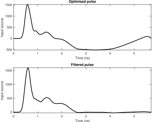
Fig. 6. The optimised pulse with and without post-processing. The low frequency component barely radiates through the antenna structure and corre-sponds to low frequency unfiltered static phenomena. To extend the pulse to more than 6 ns, the low frequency component is filtered out (filtered pulse) and subsequently zero-padding can be applied in a straightforward manner for the specified time-range.

• Source impedance (Zt)

• HDPE permittivity (h)

• HDPE conductivity (σh)

• PCB permittivity (p)

• PCB conductivity (σp)

High-density polyethylene (HDPE) material forms the skid plate and the case of the antenna, while the printed circuit board (PCB) is glass fibre on which the metal bow-ties are printed [10]. The unknowns are primarily dielectric properties, thus the Jacobian can be mainly evaluated analytically. The derivative with respect to the impedance is derived numerically using a second order finite difference scheme (see equation (25)), due to lack of an analytic expression. Similarly, if the geometrical properties were part of the optimisation parameters (e.g. flare angle of bowties, dimensions of the absorber and so on), a numerical evaluation using a finite-difference scheme can be employed to evaluate the Jacobian.

B. Post-processing

The data collected for the controlled experiments are shown in Fig. 3. All of the manufacturer’s standard post-processing filters, apart from stacking, that would normally be applied when using the 1.5 GHz antenna were disabled so that a raw response could be recorded. The only filter applied is shown in Fig. 3, and is a second order polynomial that describes low frequency current phenomena. The latter are filtered out through a simple subtraction.

C. Results

FWI is sensitive to the initial model and thus, a rational ini-tial model should be chosen in order to ensure fast convergence

TABLE I. INITIAL AND OPTIMISED ANTENNA PARAMETERS

Parameters Initial value Optimised value

Absorber-1 5 1.05

Absorber-2 5 3.96

HDPE 2.5 1.99

PCB 1.5 1.37

Absorber-1σ(S/m) 0.5 1.01 Absorber-2σ(S/m) 0.5 0.31 HDPEσ(S/m) 0.01 0.013

PCBσ(S/m) 0.001 0.0002 Zt(Ω) 75 195

22. 5 cm

36. 6 cm

26.6 cm

Fig. 7. A controlled experiment executed in order to validate the accuracy of the modelled antenna in a challenging scenario. The antenna (red) is placed on top of a hollow PEC box (grey).

and avoid local minimal. Here, the initial values were chosen based on realistic expectations of the dielectric properties of the absorbers, and the plastic elements of the antenna. For the excitation pulse, ideally a delta function should be used in order to excite the model with a wide frequency spectrum. However, when such an approach is used with the FDTD method, the result is a very noisyAmatrix which consequently creates the need for largeλ, and furthermore increasesηλ. The excitation pulse should be chosen such as to incorporate a wide spectrum of frequencies in the model while minimising the numerical error – we used the pulse suggested in [10], which is a Gaussian pulse with 1.71 GHz central frequency.

0 1 2 3 4 5

Time (ns)

-2 -1 0 1

Received field

104 Time domain

Synthetic Real

0 1 2 3 4 5 6 7

Frequency (GHz)

0 1000 2000 3000 4000 5000

Amplitude

Frequency domain

Fig. 8. Comparison between real and synthetic measurements of the experiments described in Fig. 7.

scheme should be executed for each λ. For the λ values used in the present study, the hybrid scheme converges smoothly in less than 10 iterations.

The synthetic and the real measurements for the controlled experiments are shown in Fig. 5. The modelled antenna can predict the near-field behaviour of the real antenna in a very challenging scenario, when the antenna is placed on top of a PEC.

Table I shows the initial model of the antenna and the resulting model of the hybrid linear/non-linear optimisation for λ = 1. The corresponding pulse for the parameters given in Table I is shown at Fig. 6. Due to the successful regularisation, the high frequency components associated with noise are repressed without compromising accuracy. Notice that the low frequency component of the pulse is barely radiated through the antenna structure primarily due to the small size of the bowties. Unfiltered low-frequency current phenomena are the reason that the hybrid FWI converged to the specific pulse. In order to apply the optimised pulse for a wider time range (>6ns), it is advised to filter out the low frequency component (see the filtered pulse in Fig. 6) in order to successfully zero-pad the pulse without creating sudden changes that will result in numerical errors. The measured fields using the filtered pulse have very small differences compared to the ones resulting from using the unfiltered pulse.

D. Validation

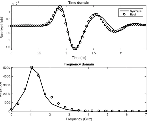
The modelled antenna is tested in two unknown scenarios which are not included in the hybrid optimisation process. The experimental setup of the first scenario is illustrated in Fig. 7. The antenna is placed on top of a hollow PEC box with dimensions 36.6 _× 26.6 _×22.5 cm. This setup was chosen in an effort to create a challenging scenario with respect to the directivity pattern. The antenna is surrounded

0 0.5 1 1.5 2

Time (ns) -1.5

-1 -0.5 0 0.5 1

Received field

104 Time domain

Synthetic Real

0 1 2 3 4 5 6 7

Frequency (GHz) 0

1000 2000 3000 4000 5000

Amplitude

Frequency domain

Fig. 9. Real and synthetic A-Scans when the antenna is coupled with dry sand.

by scattering sources, thus, an inaccurate directivity pattern will result in accumulative errors. In addition, the experiment is easily accessible and can be reproduced numerically in a straightforward manner. Fig. 7 shows the real and the synthetic measurements of the validation experiment. Both the early and the late reflections are in very good agreement indicating the validity of the modelled antenna.

The second scenario is the response of the antenna when coupled with very dry sand. The properties of the sand are chosen based on [60]. The relative permittivity is r = 2.7 and the conductivity is zero. The measurements took place in a sand box and the trace was cut at 3 ns to remove unwanted responses from the bottom of the sandbox and external sources of clutter. Fig. 9 shows the real data and the synthetic data generated using the optimised antenna model. The results are in good agreement showing that the antenna can successfully replicate near-field phenomena present in ground-coupled antennas.

IV. CONCLUSIONS

IEEE TRANSACTIONS ON GEOSCIENCE AND REMOTE SENSING 10 is now the ability to more readily include accurate models

of GPR antennas in simulations which, in turn, will provide improvements to model-based interpretations such as FWI and machine learning.

REFERENCES

[1] D. J. Daniels,Ground Penetrating Radar, 2nd ed. London, U.K.: Insti-tution of Engineering and Technology, 2004.

[2] J. M. Bourgeois and G. S. Smith, “A complete electromagnetic sim-ulation of a ground penetrating radar for mine detection: Theory and experiment,” inProc. IEEE Antennas Propag. Soc. Int. Symp., Jul. 13-18, 1997, vol. 2, pp. 986-989.

[3] D. Caratelli, A. Yarovoy, and L. P. Ligthart, “Accurate FDTD modelling of resistively-loaded bow-tie antennas for GPR applications,” in Proc. IEEE 3rd Eur. Conf. Antennas Propag.,Mar. 2009, pp. 2115-2118.

[4] S. Lambot, E. Slob, and I. van den Bosch, “Modeling of ground-penetrating radar for accurate characterization of subsurface electric properties,”IEEE Trans. Geosci. Remote Sens.,vol. 42, pp. 2555-2567, 2004.

[5] M. McFadden and W.R. Scott, “Numerical modelling of a spiral-antenna GPR system,” inProc. IEEE Int. Geosci. Remote Sens. Symp., Jul. 2009, vol. 2, pp. 109-112.

[6] K. Lee, C. C. Chen, F. L. Teixeira, and K. H. Lee, “Modeling and investigation of a geometrically complex UWB GPR antenna using FDTD,”IEEE Trans. Antennas Propag.,vol. 52, no. 8, pp. 1983-1991, Aug. 2004.

[7] L. Gurel and U. Oguz, “Three-dimensional FDTD modelling of a ground-penetrating radar,”IEEE Trans. Geosci. Remote Sens., vol. 38, no. 4, pp. 1513-1521, Jul. 2000.

[8] V. Wilson, C. Power, A. Giannopoulos, J. Gerhard, and G. Grant, “DNAPL mapping by ground penetrating radar examined via numerical simulation,”J. Appl. Geophys., vol. 69, pp. 140-149, Dec. 2009. [9] N. J. Cassidy and T. M. Millington, “The application of finite-difference

time-domain modelling for the assessment of GPR in magnetically lossy materials,”J. Appl. Geophys., vol. 67, pp. 296-308, Apr. 2009. [10] C. Warren and A. Giannopoulos, “Creating finite-difference

time-domain models of commercial ground-penetrating radar antennas using Taguchis optimisation method,”Geophysics, vol. 76, no. 2, pp. G37-G47, Apr. 2011.

[11] I. Giannakis, A. Giannopoulos, and C. Warren, “A realistic FDTD numerical modelling framework of ground penetrating radar for landmine detection,”IEEE J. Sel. Topics Appl. Earth Observ. Remote Sens., vol. 9, no. 1, pp. 37-51, 2016.

[12] C. Warren and A. Giannopoulos, “Experimental and modeled perfor-mance of a ground penetrating radar antenna in lossy dielectrics,”IEEE J. Sel. Topics Appl. Earth Obs. Remote Sens., vol. 9, no. 1, pp. 29-36, Jan. 2016.

[13] I. Giannakis, A. Giannopoulos, C. Warren, and N. Davidson, “Numeri-cal modelling and neural networks for landmine detection using ground pen- etrating radar,” inProc. Int. Workshop Adv. Ground Penetrat. Radar, Jul. 2015, pp. 1-4.

[14] K. Yee, “Numerical solution of initial boundary value problems in-volving maxwells equations in isotropic media,”IEEE Trans. Antennas Propag., vol. 14, no. 3, pp. 302-307, 1966.

[15] A. Taflove and S. C. Hagness, Computational Electrodynamics, the Finite-Difference Time-Domain Method, 2nd ed. Norwood, MA, USA: Artech House, 2000.

[16] K. L. Shlager, G. S. Smith, and J. G. Maloney, “Optimization of bowtie antennas for pulse radiation,”IEEE Trans. Antennas Propagat., vol. AP-42, pp. 975-982, 1994.

[17] J. M. Bourgeois and G. S. Smith, “Full electromagnetic simulation of a ground penetrating radar: Theory and experiment,” inProc. IEEE Antennas and Propagation Int. Symp., 1994, vol. 3, pp. 1442-1443.

[18] J. M. Bourgeois and G. S. Smith, “A fully three-dimensional simulation of ground penetrating radar: FDTD theory compared with experiment,” IEEE Trans. Geosci. Remote Sens., vol. 34, pp. 36-28, 1996.

[19] G. S. Smith, W. R. Scott, “A scale model for studying ground penetrat-ing radars,”IEEE Trans. Geosci. and Remote Sens., vol. 27, pp. 358-363, 1989.

[20] G. S. Smith and W. R. Scott, Jr., “The use of emulsions to represent dielectric materials in electromagnetic scale models,” IEEE Trans. An-tennas Propagat., vol. 38, no. 3, pp. 323-334, Mar. 1990.

[21] Z. Huang, K. R. Demarest, and R. G. Plumb, “An FDTD/MoM hydrid technique for modeling complex antennas in the presence of heterogeneous grounds,”IEEE Trans. Geosci. Remote Sens., vol. 37, no. 6, pp. 2692-2698, Nov. 1999.

[22] Z. Huang, K. R. Demarest and R. G. Plumb, “Ground penetrating radar antenna modeling.” inProc. of IEEE Geosci. and Remote Sens. Symp. (IGARSS), 1996, vol. 1, pp. 778-780.

[23] S. Lambot, E. C. Slob, M. Vanclooster, and H. Vereecken, “Closed loop GPR data inversion for soil hydraulic and electric property determina-tion,”Geophys. Res. Lett., vol. 33, pp. L21-405, 2006.

[24] K. Z. Jadoon, S. Lambot, E. C. Slob, and H. Vereecken, “Analysis of horn antenna transfer functions and phase-center position for modeling off-ground GPR,”IEEE Trans. Geosci. Remote Sens., vol. 49, no. 5, pp. 1649-1662, 2011.

[25] S. Lambot and F. Andre, Full-wave modeling of near-field radar data for planar layered media reconstruction, IEEE Trans. Geosci. Remote Sens., vol. 52, no. 5, pp. 2295-2303, May 2014.

[26] Y. Nishioka, O. Maeshima, T. Uno, and S. Adachi, “FDTD analysis of resistors-loaded bow-tie antennas covered with ferrite-coated conducting cavity for subsurface radar,”IEEE Trans. Antennas Propagat., vol. 47, no. 6, pp. 970-977, 1999.

[27] K. Holliger, B. Lampe, U. Meier, M. Lambert, and A. Green, “Realistic modeling of surface ground- penetrating radar antenna systems: where do we stand?,” inProc. of the 2nd Intern. Workshop on Advanced Ground Penetrating Radar, 2003, pp. 45-50.

[28] L. Liu, Y. Su and J. Mao, “FDTD analysis of ground-penetrating radar antennas with shields and absorbers,”Frontiers of Electrical and Electronic Engineering in China, vol. 3, pp. 90-95, 2008.

[29] L. Gurel and U. Oguz, “Simulations of ground-penetrating radars over lossy and heterogeneous grounds, IEEE Trans. Geosci. Remote Sens., vol. 39, no. 6, pp. 1190-1197, Jun. 2001.

[30] U. Oguz and L. Gurel, “Frequency responses of ground-penetrating radars operating over highly lossy grounds,” IEEE Trans. Geosci. Remote Sens., vol. 40, no. 6, pp. 1385-1394, Jun. 2002.

[31] M. A. Gonzalez-Huici and U. Uschkerat, “GPR modeling for landmine detection,” inProc. Int. Symp. Electromagn. Theory (EMTS), 2010, pp. 152-155.

[32] M. A. Gonzalez-Huici, “A strategy for landmine detection and recog-nition using simulated GPR responses,” inProc. 14th Int. Conf. Ground Penetrat. Radar (GPR), 2012, pp. 871-876.

[33] D. Uduwawala, M. Norgren, and P. Fuks, “A complete FDTD simula-tion of a real GPR antenna system operating above lossy and dispersive grounds,”Prog. Electromagn. Res., vol. 50, pp. 209-229, 2005. [34] C. Warren and A. Giannopoulos, “Investigation of the directivity of

a commercial ground-penetrating radar antenna using a finite-difference time-domain antenna model,” inProc. 14th Int. Conf. Ground Penetrat. Radar (GPR), 2012, pp. 226-231.

[35] G. Klysz, X. Ferrieres, J. Balayssac, and S. Laurens, “Simulation of direct wave propagation by numerical fdtd for a gpr coupled antenna,” NDT and E International, vol. 39, pp. 338-347, 2006.

[36] S. Xu, B. Duan and D. Zhang, “Selection of the wavenumbers k using an optimization method for the inverse Fourier transform in 2.5D electrical modelling,”Geophys. Prospect., vol. 48, no. 5, pp. 789-796, 2000.

squares optimization approach,” IEEE Trans. Antennas. Propag., vol. 55, pp. 1999-2005, 2007.

[38] A. Tarantola, “Inversion of seismic reflection data in the acoustic approximation,”Geophysics, vol. 49, no. 8, pp. 1259-1266, 1984. [39] Q. Cheng, R. Chen and T. Li, “Simultaneous wavelet estimation and

deconvolution of reflection seismic signals,”IEEE Trans. Geosci. Remote Sems.,vol. 34, no. 2, pp. 377-384, 1996.

[40] S. Busch, J. van der Kruk and H. Vereecken, “Improved characterization of fine-texture soils using on-ground GPR full-waveform inversion,” IEEE Trans. Geosci. Remote Sens., vol. 52, no. 7, pp. 3947-3958, 2014.

[41] F. A. Belina, J. Irving and J. R. Ernst, “Waveform inversion of crosshole georadar data: Influence of source wavelet variability and the suitability of a single wavelet assumption,”IEEE Trans. Geosci. Remote Sens., vol. 50, no. 11, pp. 4610-4625, 2012.

[42] F. A. Belina, J. Irving, J. R. Ernst and K. Hollinger, “Analysis of an iterative deconvolution approach for estimating the source wavelet during waveform inversion of crosshole georadar data,”J. Appl. Geophys, vol. 78, pp. 20-30, 2012.

[43] T. Liu, A. Klotzsche, M. Pondkule, H. Vereecken, J. van der Kruk and Y. Su, “Estimation of subsurface cylindrical object properties from GPR full-waveform inversion,” inProc. 9th Int. Works. on Adv. Ground Penetra. Radar (IWAGPR), 2017, pp. 1-4.

[44] R. Streich and J. van der Kruk, “Characterizing a GPR antenna system by near-field measurements,”Geophysics, vol. 72, no. 5, pp. A51-A55, 2007.

[45] A. Klotzsche, J. van der Kruk, G. A. Meles and H. Vereecken, “Cross-hole GPR full-waveform inversion of waveguides acting as preferential flow paths within aquifer systems,”Geophysics, vol. 77, pp. H57-H62, 2012.

[46] A. Kalogeropoulos, J. van der Kruk, J. Hugenschmidt, J. Bikowski, and E. Bruhwiler, “Full-waveform GPR inversion to assess chloride gradients in concrete,”NDT & E Int., vol. 57, pp. 74-84, 2013.

[47] D. Marquardt, “An algorithm for least-squares estimation of nonlinear parameters,”SIAM J. on Appl. Math., vol. 11, no. 2, pp. 431-441, 1963. [48] D. L. Phillips, “A technique for the numerical solution of certain integral equations of the first kind,”J. Assoc. Comput. Mach., vol. 9, pp. 84-97, 1962.

[49] A. N. Tikhonov, “Solution of incorrectly formulated problems and the regularization method,”Soviet Math. Dokl., vol. 151, pp. 501-504, 1963. [50] P. C. Hansen, “Analysis of discrete ill-posed problems by means of the

L-curve,”SIAM Review, vol. 34, pp. 561-580, 1992.

[51] P. C. Hansen, “The use of the L-curve in the regularization of discrete ill-posed problems,”SIAM J. Sci. Comput., vol. 14, pp. 1487-1503, 1993. [52] G. A. Meles, J. Van der Kruk, S. A. Greenhalgh, J. R. Ernst, H. Maurer, and A. G. Green, “A new vector waveform inversion algorithm for simultaneous updating of conductivity and permittivity parameters from combination crosshole/borehole-to-surface GPR data,”IEEE Trans. Geosci. Remote Sens., vol. 48, no. 9, pp. 3391-3407, 2010.

[53] P. Shangguan and I. L. Al-Qadi, “Calibration of FDTD simulation of GPR signal for asphalt pavement compaction monitoring,”IEEE Trans. Geosci. Remote Sens., vol. 53, no. 3, pp. 1538-1548, 2015.

[54] J. R. Ernst, H. Maurer, A. G. Green, and K. Holliger, “Full-waveform inversion of crosshole radar data based on 2-D finite-difference time-domain solutions of Maxwell’s equations,”IEEE Trans. Geosci. Remote Sens., vol. 45, no. 9, pp. 2807-2828, 2007.

[55] M. Moghaddam, W. C. Chew, and M. Oristaglio, “Comparison of the Born iterative method and Tarantolas method for an electromagnetic time-domain inverse problem,”Int. J. Imaging Syst. Technol., vol. 3, no. 4, pp. 318-333, 1991.

[56] J. X. Dessa and G. Pascal, “Combined traveltime and frequency-domain seismic waveform inversion: A case study on multi-offset ultrasonic data,”Geophys. J. Int., vol. 154, no. 1, pp. 117-133, 2003.

[57] K. B. Petersen and M. S. Pedersen,The Matrix Cookbook,Technical University of Denmark, version November 2012.

[58] G. A. Meles, S. A. Greenhalgh, A. G. Green, H. Maurer, and J. Van der Kruk, “GPR full-waveform sensitivity and resolution analysis using an FDTD adjoint method,”IEEE Trans. Geosci. Remote Sens., vol. 50, pp. 1881-1896, 2012.