University of Pennsylvania
ScholarlyCommons
Publicly Accessible Penn Dissertations
1-1-2014
A PDE-based Method for Optimizing Solar Cell
Performance
Xiaoxian Liu
University of Pennsylvania, [email protected]
Follow this and additional works at:http://repository.upenn.edu/edissertations
Part of theApplied Mathematics Commons,Mathematics Commons, and theMechanics of Materials Commons
This paper is posted at ScholarlyCommons.http://repository.upenn.edu/edissertations/1349
For more information, please [email protected].
Recommended Citation
Liu, Xiaoxian, "A PDE-based Method for Optimizing Solar Cell Performance" (2014).Publicly Accessible Penn Dissertations. 1349.
A PDE-based Method for Optimizing Solar Cell Performance
Abstract
In this paper, we address the optimal design problem for organic solar cells (OSC).
In particular, our focus is to enhance short-curcuit photocurrent by optimizing the
donor-acceptor interface. To that end, we propose two drift-diffusion models for
organic solar cells, both of which account for the physics of OSC's that charge
carriers are mostly generated in the region near the donor-acceptor interface. For
the first drift-diffusion model, the generation of charge carriers is translated into
a boundary condition across the donor-acceptor interface. We apply the theory of
shape optimization to compute the shape gradient functional of the photocurrent. In
particular, shape differential calculus is extensively applied in the computation. For
the second drfit-diffusion model, we parameterize the donor-acceptor interface as a
leve set of a function, i.e. the "phase field function". The dependence of the second
drift-diffusion model on the geometry is therefore transformed into its dependence
on the phase field function. Such transformation greatly simplifies the sensitivity
analysis and leads to an easy-to-implement numerical optimization algorithm. In
numerical examples, it is shown that the maximum output power of the optimized
solar cell can be increased by a factor of 3. Our analysis and examples in this paper
are in two dimensions, but the generelization of both the analysis and numerical
optimization to three dimensions is straightforward.
Degree Type
Dissertation
Degree Name
Doctor of Philosophy (PhD)
Graduate Group
First Advisor
Charles L. Epstein
Keywords
drift diffusion model, numerical optimization, partial differential equations, phase field method, shape optimization, solar cells
Subject Categories
A PDE-BASED METHOD FOR OPTIMIZING SOLAR CELL
PERFORMANCE
Xiaoxian Liu
A DISSERTATION
in
Applied Mathematics and Computational Sciences
Presented to the Faculties of the University of Pennsylvania in Partial
Fulfillment of the Requirements for the Degree of Doctor of Philosophy
2014
Charles L. Epstein, Thomas A. Scott Professor of Mathematics
Supervisor of Dissertation
Charles L. Epstein, Thomas A. Scott Professor of Mathematics
Graduate Group Chairperson
Dissertation Committee:
Cherie R. Kagan, Professor of Material Science and Engineering
Eugene J. Mel´
e, Professor of Physics and Astronomy
Acknowledgments
First of all, my special thanks go to my adviser, Dr. Epstein, for his encouragement
and patience ever since my first day at Penn. The discussions we had have been
absolutely indispensable for my research. This work would not have been possible
without his guidance and help along the way.
I thank Dr. Kagan and Dr. Mel´e for the hours of discussion they spent with
me. It has greatly deepened my understanding of semiconductor devices and has
made my research experience so much more enjoyable. I also thank everyone in Dr.
Kagan’s group, especially Dr. Aaron Fafarman, for all the helpful discussions, even
on the topics that are completely trivial to them.
I thank Dr. Andreas Kl¨ockner, whom I met when I was a visiting student at the
Courant Institute of New York University. Without his help, it would have been so
much more difficult to build efficient numerical solvers.
I would like to extend my thanks to all of my fellow AMCS students and other
people I have met at Penn. You all have made my life at Penn as vivid as it has
I would like to thank my families. They are the dearest people to me. My
parents, who are my biggest supporters, help me through many difficulties. I wish
I could always make them proud. And to my lovely wife, I just want to say that
meeting you is the best thing that has happened to me in the past 5 years.
Finally, I thank the NSF grants DMS-0935165 and DMS-1205851 for supporting
ABSTRACT
A PDE-BASED METHOD FOR OPTIMIZING SOLAR CELL PERFORMANCE
Xiaoxian Liu
Charles L. Epstein
In this paper, we address the optimal design problem for organic solar cells (OSC).
In particular, our focus is to enhance short-curcuit photocurrent by optimizing the
donor-acceptor interface. To that end, we propose two drift-diffusion models for
organic solar cells, both of which account for the physics of OSC’s that charge
carriers are mostly generated in the region near the donor-acceptor interface. For
the first drift-diffusion model, the generation of charge carriers is translated into
a boundary condition across the donor-acceptor interface. We apply the theory of
shape optimization to compute the shape gradient functional of the photocurrent. In
particular, shape differential calculus is extensively applied in the computation. For
the second drfit-diffusion model, we parameterize the donor-acceptor interface as a
leve set of a function, i.e. the “phase field function”. The dependence of the second
drift-diffusion model on the geometry is therefore transformed into its dependence
on the phase field function. Such transformation greatly simplifies the sensitivity
analysis and leads to an easy-to-implement numerical optimization algorithm. In
numerical examples, it is shown that the maximum output power of the optimized
are in two dimensions, but the generelization of both the analysis and numerical
Contents
1 Introduction 1
1.1 Physics of Organic Solar Cells . . . 1
1.2 Mathematical Modeling of Semiconductor Devices . . . 3
1.2.1 A hierachy of existing models . . . 3
1.2.2 Drift-diffusion model for organic solar cells . . . 4
1.3 Optimal Morphology . . . 5
1.3.1 What is optimal morphology? . . . 5
1.3.2 Optimal control with drift-diffusion equations . . . 6
1.4 Two Drift-Diffusion Models for the Optimal Design of Organic Solar Cells . . . 7
1.4.1 The first drift-diffusion model: sharp donor-acceptor interface and shape optimization . . . 7
1.4.2 The second drift-diffusion model: phase field method . . . . 8
2 Optimal Control with PDE Constraints 11
2.1 Statement of an Optimal Control Problem of Partial Differnetial
Equations . . . 12
2.2 Sensitivity Analysis of Optimal Control Problems . . . 14
2.3 First-order Optimality Condition . . . 16
2.4 Example: Optimal Control of Poisson Equation . . . 20
2.5 Overture to Optimal Design of Organic Solar Cells . . . 22
3 First Drift-Diffusion Model: zero-width interface 25 3.1 Geometry of organic solar cells: zero-width interface . . . 26
3.2 Drift-diffusion equations . . . 27
3.2.1 Assumptions . . . 28
3.2.2 Boundary value problems of organic solar cells . . . 30
3.2.3 Modeling of parameters . . . 33
4 Shape Differential Calculus 36 4.1 Tangential Differential Calculus . . . 37
4.2 Signed Distance Function . . . 39
4.3 Speed Method . . . 40
4.4 Shape Derivative of a Function . . . 41
4.5 Shape Derivative of a Functional . . . 45
4.7 Example of Shape Optimization . . . 48
5 Shape Optimization with Drift-Diffusion Model 55 5.1 Admissible Velocity Field . . . 56
5.2 Preparation on Notations . . . 58
5.3 Shape Sensitivity Analysis of Drift-Diffusion Model . . . 59
5.3.1 Shape sensitivity of physical parameters . . . 60
5.3.2 Shape sensitivity of Dirichlet boundary conditions on ΓD . . 63
5.3.3 Shape sensitivity of function values on Γ . . . 64
5.3.4 Shape sensitivity of PDE’s in Ω1∪Ω2 and shape sensitivity of flux boundary conditions on ΓN ∪Γ . . . 65
5.3.5 Summary of boundary value problems for {ψ0, n0, p0, u0} . . . 65
5.4 Shape Gradient of Photocurrent and the First Order Optimality Con-dition . . . 68
5.4.1 Shape derivative of photocurrent J0 . . . 68
5.4.2 Adjoint equations and the Lagrangian functional . . . 68
5.4.3 Shape gradient . . . 73
6 Second Drift-Diffusion Model: the Phase-Field Method 75 6.1 Introduction to Phase Field Method . . . 77
6.1.1 Example: mean curvature flow . . . 78
6.1.3 Optimal design with phase field method . . . 83
6.2 Phase-Field Drift-Diffusion Model . . . 85
6.2.1 Drift-diffusion model . . . 85
6.2.2 Boundary value problem for the phase field function of an organic solar cell . . . 89
6.3 Sensitivity Analysis of Phase Field Model . . . 90
6.3.1 Sensitivity of parameters . . . 91
6.3.2 Sensitivity of drift-diffusion equations . . . 93
6.4 Phase-Field Gradient and First-Order Optimality Condition . . . . 95
6.5 Optimization Algorithm . . . 103
7 Numerical Optimization with the Phase-Field Drift-Diffusion Model106 7.1 Numerical Methods for Solving Partial Differential Equations . . . . 106
7.1.1 Mesh for numerical solutions . . . 107
7.1.2 Numerical method for solving state equations . . . 107
7.1.3 Numerical method for solving adjoint equations . . . 113
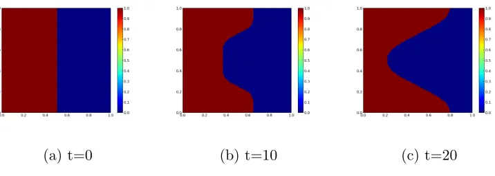
7.1.4 Numerical method for solving the Allen-Cahn equation . . . 116
7.2 Numerical values for physical parameters . . . 118
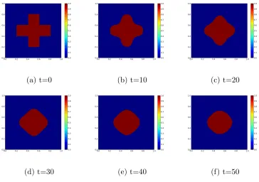
7.3 Numerical Examples . . . 121
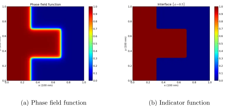
7.3.1 An example of a phase field function . . . 121
7.3.2 Solutions to the phase-field drift-diffusion model . . . 123
7.4 Discussion . . . 139
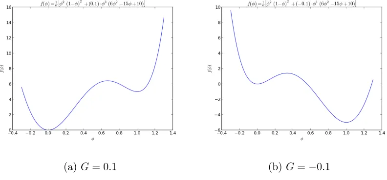
7.4.1 Amplitude of G . . . 139
7.4.2 Interface length v.s. domain connectivity . . . 142
7.4.3 Phase parameters κ . . . 147
8 Conclusion 150 Appendices 153 A Shape Sensitivity of the First Drift-Diffusion Model 154 A.1 Shape sensitivity of ψ-equation . . . 155
A.2 Shape sensitivity of n-equation . . . 158
A.3 Shape sensitivity of p-equation . . . 160
A.4 Shape sensitivity of u-equation . . . 162
B Adjoint Equations of Shape Optimization for the First Drift-Diffusion Model 164 C Sensitivity Analysis of Phase-Field Drift-Diffusion Model 180 C.1 Shape Sensitivity of ψ-equation . . . 181
C.2 Shape Sensitivity of n-equation . . . 182
C.3 Shape Sensitivity of p-equation . . . 183
Chapter 1
Introduction
Organic solar cells (a.k.a.OSCs) have emerged as a promising candidate for future
solar cells, mostly due to its low cost to manufacture. However, the efficiency of
power conversion of current experimentally available OSCs is barely above 10%,
much lower than that of inorganic solar cells [28]. It is therefore important to
improve the efficiency of OSCs, which is what we are trying to address in this work.
1.1
Physics of Organic Solar Cells
A typical OSC is comprised of two different organic materials, known as the “donor”(D)
and “acceptor”(A). Both donor and acceptor are characterized by their electronic
structures, in particular the highest occupied molecular orbital (a.k.a. “HOMO”)
and the lowest unoccupied molecular orbital (a.k.a. “LUMO”). They are the analog
as silicon.
When light is absorbed by organic polymers, an electron in the HOMO state is
excited to reach the LUMO state, and at the same time a hole (regarded as
posi-tively charged particle) is created in the HOMO state. Due to the strong Coulomb
attraction between the electron and the hole, they are closely bound together. Such
bound pairs of electrons and holes are treated as a charge neutral particles called
“excitons”. This is in contrast to the case of inorganic semiconductors, where the
Coulomb potential between electrons and holes is so weak that electrons and holes
are effectively treated as free particles after photo excitation.
Excitons are essentially an excited electronic state and they have, on average,
finite life time. Before their decay, excitons move inside either donor or acceptor by
diffusion. Excitons can also dissociate into free electrons and holes. The key feature
of the exciton dissociation is that it mainly takes place near the donor-acceptor
interface. Hence, it is not surprising that the performance of OSC’s is greatly
influenced by its morphology, i.e. the spatial distribution of donor material and
acceptor material. Once excitons arrive at the DA interface, due to the difference
in the energy levels of LUMO and HOMO, electrons and holes tend to stay in their
energetically favorable states, which leaves the electron in the acceptor and the hole
Figure 1.1: Exciton dissociation and charge transport near donor-acceptor interface.
The diagram is extracted from the paper [6].
1.2
Mathematical Modeling of Semiconductor
De-vices
1.2.1
A hierachy of existing models
There are a family of mathematical models for the transport properties of
semi-conductors [22, 18]. They can be roughly divided into two categories:
micro-scopic models and macromicro-scopic models. Micromicro-scopic dynamics of electrons can be
modeled either classically by the Liouville’s equation or quantum mechanically by
Schr¨odinger’s equation or the density matrix operator. To address the dynamics of
equation based on those microscopic models. Nonetheless, it is computationally
costly to use either microscopic models or the Boltzman equation, however
accu-rate they are, and it leads to the need for macroscopic models. In contrast, the
macroscopic models of semiconductors are concerned with macroscopic quantities,
such as electrical potential and spatial densities of charge carriers. In terms of
computational cost, they are more accessible than Boltzmann equation.
1.2.2
Drift-diffusion model for organic solar cells
The mathematical model that we use in this work is based on the drift-diffusion
equations, a macroscopic PDE model. Conventional drift-diffusion equations include
a Poisson’s equation for the electrical potential and reaction-diffusion equations for
the density functions of electrons and holes. It has proved successful on modeling
semiconductor devices in the past few of decades; in fact, it can be formally derived
from the Boltzmann equation under certain assumptions [22]. Questions on the
existence and uniqueness of such system are now well understood [21, 22, 17].
For OSC’s, one needs to extend the conventional drift-diffusion model by adding
a reaction-diffusion equation for excitons. Furthermore, as pointed out in Sec. 1.1,
it is essential to include the dependence of reaction rates on the morphology of
OSC’s. A few drift-diffusion models for OSCs have been proposed in previous works
[1, 19, 5, 6, 12, 11, 3]. In particular, [1, 19] proposed one-dimensional drift-diffusion
The influence of morphology of OSC’s on its performance is investigated from a
computational point of view. Mathematical analysis of drift-diffusion equations in
OSCs was first addressed in [12].
1.3
Optimal Morphology
1.3.1
What is optimal morphology?
In the aforementioned works on drift-diffusion models for OSC’s, much emphasis
has been given to the modeling of physical parameters such as carrier mobilities,
dissociation rate of excitons, and recombination rate of electrons and holes. These
results laid the groundwork for the drift-diffusion model for OSC’s, but the quest
for optimal morphology was not resolved.
In [5, 6], an optimal design was postulated. By numerically solving the
drift-diffusion equations, it is observed that OSC’s with such “optimal” design exhibits
better performance than those with planar D-A interface. However, such
“opti-mality” is not defined with mathematical rigor; in fact, it’s not clear whether the
postulated design can be further optimized. In this work, it is our goal to uncover
the optimality condition on morphology. In other words, we would like to improve
1.3.2
Optimal control with drift-diffusion equations
The first work on optimal design with drift-diffusion model is [15]. Unlike the
ap-proach of band structure engineering, the authors of this paper view the dopant
density as a control function and introduced the optimal control theory to
semi-conductor design. The same authors gave a summary of the optimal design with
drift-diffusion model in [16]. Furthermore, [27] extended the optimal control
frame-work to quantum drift-diffusion model.
Our analysis and computation in this work is similar to [15] in that it is also
an application of the optimal control theory on the drift-diffusion model. However,
the specific optimization problem is quite different from that in [15]. On the one
hand, the drift-diffusion model of organic semiconductors is very different from
its counterpart for conventional semiconductors. On the other hand, the control
function is not explicitly present in the model: since the goal is to identify the
optimal geomtry of the donor-acceptor interface, our control must be the geometry
itself or a representation of the geometry. Therefore, our primary goal is to formulate
the drift-diffusion model in such a way that its dependence on the geometry is
“easily” tractable.
We also note that, the idea of geometric optimization may also be applicable
to conventional semiconductors. In fact, we can transform the work of [15] to
following form
C=Cp1p+Cn1n (1.3.1)
whereCp,nare the constants of dopant densities and1p,nare the indicator functions
of the p-side and n-side of a PN junction, respectively. Unlike [15], the interest here
is the optimal indicator function 1p and 1n, i.e. the optimal layout of materials
for a PN junction. Even though the generation of electrons and holes are not
strongly associated with the interface of a PN junction, we expect the dependence
of solutions on the layout of C through the drift-diffusion model.
1.4
Two Drift-Diffusion Models for the Optimal
Design of Organic Solar Cells
1.4.1
The first drift-diffusion model: sharp donor-acceptor
interface and shape optimization
As pointed out in Section 1.1, most of the free charge carriers are generated in
a very narrow neighborhood of the donor-acceptor interface. The width of such
region is only a few percent of the dimension of the whole solar cell. When it
comes to mathematical modeling, it makes sense to take the limit of zero-width
for the interfacial region which leads to our first drift-diffusion model where all the
on the interface. By taking this limit, one can focus on the geometry of the interface
and analyze its influence on the performance of the solar cell.
Once such limit is taken, the optimal design problem falls into the regime of
shape optimization, which is prevalent in such fields as structural optimization in
mechanical engineering. We introduce the theory of shape differential calculus and
then apply it to the shape optimization problem of our first drift-diffusion model.
As is shown later, although shape optimization is conceptually easy, the analysis
of shape optimization is in general harder than ordinary optimization problems.
Statement of the first drift-diffusion model and the shape optimization analysis of
it can be found in Chapter 3 -5.
1.4.2
The second drift-diffusion model: phase field method
A few difficulties arise in the shape optimization approach above. First of all,
the formulations of the adjoint equations and the shape gradient functional are
very complicated and appear to be difficult for both analytical and computational
purposes. Also, optimal shapes are in general expected to be very complex. Explicit
parametrization of D-A interface leads to several difficulties in computation. For
instance, it is difficult to handle topological change via explicit parametrization of
shape boundary. Furthermore, one needs to resolve the issue of remeshing for each
updated shape.
interface is assumed to be the level set of some function defined on the whole domain.
Such a viewpoint leads us to the second drift-diffusion model. To be specific, we first
introduce a level set function called the “phase field function” φ. Given any phase
field function φ, we can write down the drift-diffusion equations whose dependence
on the geometry is expressed by the dependence of all the modeling parameters on
φ. For example, if we have a Poisson equation with a diffusivity coefficient D,
−∇ ·(D∇y) =f
its formulation, based on level set function, is
−∇ ·(D(φ)∇y) =f(φ)
Such an approach provides certain convenience for our purpose. On the one
hand, the adjoint equations and the gradient functional for this phase field model
are much simpler, compared with the adjoint equations and shape gradient in the
approach of shape optimization. On the other hand, the numerical implementation
of the phase-field method is much easier: instead of updating the geometry for
each step and remeshing the whole domain, we can solve the equations on a fixed
rectangular grid without the overhead of remeshing, and the evolution of shape is
1.5
Summary of Later Chapters
In Chapter 2, we start by introducing the theory of optimal control with PDE
constraints, which is the standard method of solving optimization problems for
PDE’s and used in both drift-diffusion models.
From Chapter 3 to Chapter 5, we concentrate on the first drift-diffusion model
and the shape optimization problem. For completeness, useful results of shape
dif-ferential calculus are introduced in Chapter 4. We conclude Chapter 5 by computing
the shape gradient functional of photocurrent.
Chapter 6 and 7 are dedicated to the second drift-diffusion model based on the
phase field method. In Chapter 6, we introduce the second drift-diffusion model and
apply sensitivity analysis to it. In particular, we compute the phase-field gradient
functionalGand state an optimization algorithm based on the Allen-Cahn equation.
In Chapter 7, we provide details of the numerical methods for solving each partial
differential equation of the optimization algorithm, and conclude the chapter with
Chapter 2
Optimal Control with PDE
Constraints
Before entering the details of optimal design of organic solar cells, let us briefly
review the mathematics of optimal control of partial differential equations, which
is applied repeatedly in later chapters. The purpose is to present a high-level
introduction to optimal control so that later chapters are more accessible to the
readers. Therefore, we focus on the formulation of optimal control in a PDE setting
and its sensitivity analysis; we do not worry about the mathematical topics such
as the existence and even uniqueness of optimal solution, albeit their importance is
evident. Many references are available on the theory of optimal control of PDE’s,
2.1
Statement of an Optimal Control Problem of
Partial Differnetial Equations
To define an optimal control problem, we need to introduce the basic concepts of
functional analysis. Let V and U be two Banach spaces. We keep the convention
that V is the space ofstate functionsorstate variablesandU is the space ofcontrol
functions or control variables; both concepts are made clear later.
A bounded linear functionall :V 7→Ris a linear function that maps all elements inV to the set of real numbers. The vector space of bounded linear functionals on a
Banach space is called its dual space. The dual spaces ofV andU are denoted asV∗
and U∗, respectively. We assume both V and U are reflexive, meaning (V∗)∗ =V
and (U∗)∗ = U. The action of a functional l ∈ V∗ on a function y ∈ V is often
written as
l(y) =< l, y >(V∗,V) ∈R (2.1.1)
It looks very much like an inner product on a Hilbert spaces. In fact, if V is a
Hilbert space, that is, a Banach space with an inner product structure, V∗ can be
identified with V, and (2.1.1) is indeed an inner product.
Lety∈V be our state variable and u∈Uad ⊂U be our control variable. Uad is
a closed subset ofU, and is called theadmissiblesubset of U; we are only interested
in the control functions in Uad. The relationship between y and u is determined
abstract level, we can formally write this PDE model as
A(y) =B(u) (2.1.2)
where A :V 7→ V∗ and B :Uad 7→ V∗ are two operators that map y and u to the
same element in V∗. Note thatA(y) =B(u) does not have to be linear PDE’s; both
AandB can possibly depend onyandu, and in such case we have a nonlinear PDE
model. We always assume the equation A(y) = B(u) is well defined for ∀u ∈ Uad.
Alternatively, we can define a solution operator S : U 7→ V such that y = S(u) is
the solution to A(y) =B(u).
An analogy in linear algebra may help to understand the dry statements so far.
Concretely, one can think ofV as a finite-dimensional Eucledian spaceRn: V is the
space of column vectors, andV∗is the space of row vectors (dual of column vectors).
The pairing between V and V∗ is simply the dot product of Eucledian space. The
same analogy holds for U. Our state variable y and control variable u are column
vectors living in V and U, respectively. The operators A and B are represented
as n-by-n and n-by-m matrices, respectively. In other words, the finite-dimensional
analogue of our PDE model A(y) = B(u) is a system of algebraic equations.
Having defined state variableand control variable and the function spaces they
belong to, we are ready to formulate an optimal control problem with PDE
smooth function ofy and u. The corresponding optimal control problem with PDE
constraints can be formulated as
min
u∈Uad
J[y(u), u] (2.1.3)
where A(y) =B(u) (2.1.4)
2.2
Sensitivity Analysis of Optimal Control
Prob-lems
The purpose of sensitivity analysis is to understand how the state functionyand the
cost functionalJ are affected by changef to control functionu. To this end, we need
to introduce the notion of Gˆateaux differentiability and Fr´echet differentiability in
function space. We let u∈U and y(u)∈V be two elements in two Banach spaces.
Definition 2.2.1 (Directional derivative). The first variation of the state function
y(u) in the direction of u1 ∈U is
y0(u;u1) d
= lim
t→0+
y(u+tu1)−y(u)
t (2.2.1)
if the limit exists in V and u+tu1 ∈Uad for∀t ∈[0, ) ( >0).
Definition 2.2.2(Gˆateaux differentiable). Suppose the directional derivativey0(u;u1)
exists for ∀u∈Uad,∀u1 ∈U. If there exists a continuous linear operatorMG :U 7→
V such that
for all admissible u1 ∈U, then the mapy(u) :Uad 7→V is Gˆateaux differentiable at
u and the linear operator MG is the Gˆateaux derivative of y(u).
Definition 2.2.3 (Fr´echet differentiable). y(u) is Fr´echet differentiable atuif there
exist a continuous linear map MF :U 7→V such that
lim
ku1kU→0
ky(u+u1)−y(u)−MFu1kV
ku1kU
= 0 (2.2.3)
for ∀u1 ∈ U. The Fr´echet derivative of y(u) at u is therefore defined to be the
operator MF.
Remark 2.2.4 (Gˆateaux derivative v.s. Frˆechet derivative). Fr´echet differentiability
is a stronger requirement: Gˆateaux differentiability only guarantees differentiability
in the sense of linear purturbation, whereas Fr´echet differentiable defines uniform
differentiability for all possible ways of taking the limit. If a function is Fr´echet
differentiable, then it is Gˆateaux differentiable and its Fr´echet derivative is also its
Gˆateaux derivative; the reverse is in general false.
Remark 2.2.5 (Notation on derivatives). For our purpose, we shall mostly work with
Gˆateaux derivative; sometimes it’s even sufficient to only look at directional
deriva-tives for all the admissible directions. Therefore we make the following convention
Directional derivative: y0(u;u1) or y0 (2.2.4)
Gˆateaux derivative: ∂y
Now we are in place to introduce the sensitivity of state equationA(y) =B(u)
and the cost functional J. We shall assume y(u) is always Gˆateaux differentiable
with respect to u and J(y, u) is Gˆateaux differentiable with respect to both y and
u. Then, formally, we have
• Sensitivity of the state equation A(y) =B(u)
The directional derivative y0(u;u1) satisfies the following linear equation
Ay y0(u;u1) = Buu1 (2.2.6)
Here Ay is the formal derivative of A with respect to y, which is a linear
operator, and we have similar assertion on Bu
• Sensitivity of the cost functional J[y(u), u]
By the chain rule, it is easy to obtain the sensitivity of J with respect to u
J0[y(u), u;u1] =<
∂J ∂y, y
0(u;u
1)>V∗,V +<
∂J
∂u, u1 >U∗,U (2.2.7)
where ∂J∂y and ∂J∂u are the Gˆateaux derivative of J with respect to y and u;
they are apparently functionals in V∗ and U∗, respectively.
2.3
First-order Optimality Condition
For optimal control problem, one is often interested in the optimality condition
for J as a function of u. Thus the sensitivity of J in y, i.e. ∂J∂y ∈ V∗ needs to
adjoint equations, and the most convenient way of deriving the adjoint equations is
by forming the Lagrangian functional L.
We first define the adjoint of a linear operator. Let A : V 7→ U be a bounded
linear operator. We also let l be a linear functional in U∗ and let y be a vector in
V. Then we can define theadjoint operator A∗ :U∗ 7→V∗
< l, Ay >(U∗,U)=< A∗l, y >(V∗,V) (2.3.1)
Now we let p∈V and then construct theLagrangian functionalL as
L(y, u, p) =J(y, u)−< A(y)−B(u), p >(V∗,V) (2.3.2)
The function p is the so-called Lagrange multiplier or adjoint variable. Note that
although L is in general a nonlinear functional ofy andu, it is linear in the adjoint
variable p.
NowL(y, u, p) :V×Uad×V 7→Ris a smooth function iny,u,andp, and therefore
we can consider its sensitivity with respect to the control variable u. Since p does
not depend on u, we have
L0(y, u, p;u1) =<
∂J ∂y, y
0
(u;u1)>V∗,V +<
∂J
∂u, u1 >U∗,U
−< Ayy0(u;u1)−Buu1, p >V∗,V
=< ∂J ∂y −A
∗ yp, y
0
(u;u1)>V∗,V
+< ∂J ∂u +B
∗
u p, u1 >U∗,U (2.3.3)
L0 is apparently linear in y0(u;u
1) and u1. Furthermore, we have the freedom of
the adjoint equation inV∗
A∗yp= ∂J
∂y (2.3.4)
we end up with
L0(y, u, p;u1) =<
∂J ∂u +B
∗
u p, u1 >U∗,U
=< ∂J
∂u, u1 >U∗,U +< Buu1, p >V∗,V
=< ∂J
∂u, u1 >U∗,U +< Ay y
0
(u;u1), p >V∗,V
=< ∂J
∂u, u1 >U∗,U +< A
∗ yp, y
0
(u;u1)>V∗,V
=< ∂J
∂u, u1 >U∗,U +< ∂J ∂y, y
0
(u;u1)>V∗,V
=J0(y, u;u1) (2.3.5)
i.e. we have recovered the sensitivity of J and have effectively defined the gradient
functional of J with respect tou by
G(y, u, p) = ∂J ∂u +B
∗ up∈U
∗
(2.3.6)
which is the main purpose of our sensitivity analysis. Thus we can summarize the
first-order optimality condition: if y and u solves the state equation A(y) = B(u)
and psolves theadjoint equationA∗yp= ∂J∂y then the necessary first-order optimality
condition at (y, u) is
J0(y, u;u1) =< G(y, u, p), u1 >U∗,U ≥0 (2.3.7)
where G(y, u, p) = ∂J ∂u +B
∗ up
for all the admissible u1 ∈U.
An important observation is that the method of adjoint equation does not only
help us identify the optimality condition, but also helps to compute the gradient
functional G, which in turn provides analytical tools for numerical methods of
solving for some optimal control ¯u.
Remark 2.3.1 (Formulation of Lagrangian functional). Previously we formulate the
Lagrangian functional as in (2.3.2). In fact, for equality constraints (such as PDE’s),
we can form a Lagrangian differently, i.e.
L(y, u, η) =J(y, u) +hA(y)−B(u), ηi (2.3.9)
The only difference is that we use “+” instead of the “-” in (2.3.2). This of course
leads to a different adjoint equation, but it’s easy to see the two adjoint variables
have the simple relationship η = −ξ. One can use either (2.3.2) or (2.3.9) to
2.4
Example: Optimal Control of Poisson
Equa-tion
Let Ω be a connected domain in R2 whose boundary is Lipschitz. We consider the
following optimization problem
min
u∈L2(Ω)J = Z
Ω
1
2(y−yd)
2 (2.4.1)
where − ∇2y=u Ω (2.4.2)
y= 0 ∂Ω
where yd is a known function in L2(Ω). The PDE is a simple Poisson’s equation
with homogeneous Dirichlet boundary condition in R2. Our goal is to identify the first order optimality condition of J with respect to the controlu.
We let both the space of control functionsU and the space of state functionsV to
be the Sobolev spaceL2(Ω). Basic theory of PDE tells us, for a givenu∈L2(Ω), we
have a unique state solutiony∈H1
0(Ω)⊂L2(Ω). We further letp∈H1(Ω)⊂L2(Ω)
be the Lagrange multiplier and write the Laplace equation in its weak form
Z
Ω
∇y· ∇p−
Z
∂Ω
∂y ∂νp=
Z
Ω
u p (2.4.3)
We then form the Lagrangian functional as
L(y, u, p) = Z
Ω
1
2(y−yd)
2 −
Z
Ω
∇y· ∇p+ Z
∂Ω
∂y ∂νp+
Z
Ω
u p (2.4.4)
form the Lagrangian functional, because the classical solution to −∇2y = u does
not exist in general when u only has L2 regularity.
To apply sensitivity analysis to the state equation, we proceed by formally taking
directional derivatives on (2.4.3) as well as the Dirichlet boundary condition in the
direction ofu1 ∈L2(Ω). After an integration by parts, we end up with the following
boundary value problem
− ∇2y0
=u1 Ω (2.4.5)
y0 = 0 ∂Ω (2.4.6)
It’s not hard to show that there is a unique solutiony0(u;u1)∈H01(Ω) ⊂L2(Ω). One
can even make one step further to show that y(u) is in fact Gˆateaux differentiable
in V =H01(Ω) with respect tou∈L2(Ω).
Next we compute the directional derivative ofL. For ∀u1 ∈U,
L0(y, u, p;u1) =
Z
Ω
(y−yd)y0(u;u1)−
Z
Ω
∇p· ∇y0(u;u1) +
Z
∂Ω
∂y0(u;u1)
∂ν p
+ Z
Ω
p u1 (2.4.7)
By applying integration by parts to the first line of the right hand side we
obtained the adjoint equation for p
− ∇2p=y−y
d Ω (2.4.8)
p= 0 ∂Ω (2.4.9)
Note that the adjoint equation above shows that p is in fact also a function in
H1
Finally, we summarize the sensitivity ofJ with respect to the control variableu
J0(y, u;u1) =< p, u1 >L2(Ω)= Z
Ω
p u1 (2.4.10)
where the gradient functional is simply
G=p∈L2(Ω) (2.4.11)
The necessary optimality condition for an unconstrained problem is simplyG=
0. Hence for this simple problem, we have
p∗ = 0 (2.4.12)
where p∗ is the adjoint function inH1(Ω) corresponding to the optimal solutiony∗.
Sincep∗ must satisfy the adjoint equation, it is easy to see that the optimal solution
is
y∗ =yd (2.4.13)
in L2(Ω), and the minimum value for cost functional J is 0.
2.5
Overture to Optimal Design of Organic Solar
Cells
Conceptually, it is not hard to translate the optimal design problem of organic
solar cells into the framework of optimal control with PDE constraints. Suppose
drift-diffusion equations whose solution is denoted asy, Then we can view the
donor-acceptor interface Γ as the “control variable” which affects the value of J through
the drift-diffusion equations. But the subtle question here is how to represent the
geometry?
In later chapters, we present two views of the geometry of organic solar cells,
which leads to two different versions of the drift-diffusion model.
• Drift-diffusion model 1: zero-width donor-acceptor interface (cf. Chapter 3
-5)
In the first model, we take a shape optimizationapproach and view the
donor-acceptor interface as a zero-width boundary between the two materials. By
defining proper boundary conditions on Γ, we effectively define the map from
Γ to y. To find the optimality condition of Γ, we need to understand the
sensitivity of y with respect to Γ. To this end, we need to introduce tools of
shape differential calculus.
• Drift-diffusion model 2: phase-field method (cf. Chapter 6 - 7)
The second drift-diffusion model is based on a level-set approach. We
intro-duce thephase field function φas a level set function and the level set defined
byφ= 0.5 is assumed to be the donor-acceptor interface Γ; in other words, we
replace Γ byφas thecontrol. As a result, all the parameters and coefficients of
the drift-diffusion model depend onφ, and thus we have made the dependence
that the numerical implementation of this approach is rather straightforward
Chapter 3
First Drift-Diffusion Model:
zero-width interface
In this section, we introduce the drift-diffusion equations that are used to model
organic solar cells. A few papers have been published on drift-diffusion model in
organic solar cells. For example, see [1, 6, 11]. In these works, specific models for
carrier mobilities and the dissociation rates of excitons have been discussed.
Al-though the modeling of such physical parameters is of fundamental importance, the
focus of this paper is to understand the influence of shape on the carrier transport
properties. Thus we only make some general and reasonable assumptions on these
physical parameters.
In what follows, we introduce the geometry of the device first. And then we
assumptions and mathematical formulations.
3.1
Geometry of organic solar cells: zero-width
interface
Organic solar cells are made up of two materials, known as the donor and the
ac-ceptor. We use ”1” to indicate the donor phase and ”2” to indicate the acceptor
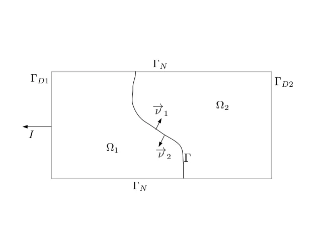
phase. A two-dimensional example is given in 3.1
• domain
Let Ω ∈Rd, d = 2,3 be a rectangular open region. Let Ω
1 ⊂ Ω and Ω2 ⊂ Ω
be two smooth open subregions such that Ω = Ω1∪Ω2 and Ω1∩Ω2 =∅.
• exterior boundaries
Let∂Ω1 and ∂Ω2 be the boundary of Ω1 and Ω2, respectively. In addition, we
require a side of Ω is part of ∂Ω1, denoted as ΓD1 and another disconnected
side is part of∂Ω2, denoted as ΓD2. From a physical perspective, ΓD1and ΓD2
are two contacts connected to different electrodes; apparently they must be
disconnected, because otherwise the two contacts are short-circuited. We also
define ΓN =∂Ω\(ΓD1∪ΓD2). It represents the parts of the boundary where
a zero flux boundary condition or a periodic boundary condition is defined.
• interface
We define the interface as Γ = ∂Ω1∩∂Ω2. Γ is supposed to be smooth, but it
does not have to be connected.
We use ν to denote outward normal vector for the whole domain. On the interface
Γ, we use ν1,2 for the outward normal vector for Ω1,2, respectively.
3.2
Drift-diffusion equations
For solar cells, we’re interested in the stationary case where the photo current and
equations, where we solve for the following unknowns:
ψ Electric potential
n Electron density
p Hole density
u Exciton density
We first describe the basic assumptions of the model and then state the boundary
value problem explicitly.
3.2.1
Assumptions
• Reactions
Symbolically, we use (e−, h+) for excitons and e− and h+ for electrons and
holes. We assume there are only 3 reactions that need to be addressed in the
model.
1. All the incoming photons (light) are converted to excitons (e−, h+) with
rate Q. HereQ is a function of spatial variables, but it does not depend
on the design of OSCs.
2. There is a bi-directional reaction between excitons and free carriers:
exci-tons may dissociate into free electrons and holes, and electrons and holes
can also recombine to form excitons. We use f for the net production
rate of free carriers, i.e. f is the rate of exciton dissociation minus the
3. Excitons have a chance to decay into other forms of energy, which do not
lead to the formation of charge carriers any more. We assume its rate
takes the intuitive form duu, where τu = 1/du has the physical meaning
of average lifetime of excitons.
All three reactions are summarized in the table below.
Type of Reaction Reaction Rate
light−→(e−, h+) Q
(e−, h+)e−+h+ f
(e−, h+)−→thermal energy +... d uu
Remark 3.2.1. Omission of “triplet excitons”
In principle, there are two types of excitons that need to be considered: the
“singlets” (spin 0) and the “triplets” (spin 1). In the previous models such as
[6, 11], it was pointed out that carrier recombination can lead to the
forma-tion of both “singlets” and “triplets”, and yet it is the “singlets” that are of
interest. Therefore, in these models we have
Net conversion of singlet excitons: ku−αγnp
Net production of charge carriers: ku−γnp
wherek is the dissociation coefficient of excitons, γ is the recombination
coef-ficient of charge carriers, and α is the fraction of singlets produced by carrier
In this work, we do not differentiate between the “singlets” and “triplets” for
simplicity, i.e. we usef for both the net conversion rate of excitons to carriers
and the net production rate of carriers; cf. Section 3.2.2. The presence of
“triplets” can be enforced by a modification of the boundary value problems
in Section 3.2.2, but we choose not to do so for simplicity.
• Zero-width interface
The physics of organic solar cells indicates that the reactions among electrons,
holes, and excitons mainly take place near the donor-acceptor interface. The
width of this “active” region is relatively small compared with the dimension
of the device. In this paper, we take the limit of this width going to 0. In
other words, all reactions are assumed to take place strictly on the interface.
In mathematical terms, this is simply translated to a boundary condition on
the interface as shown in Section 3.2.2. Such an assumption was also made in
[11], where it is referred to as a “coarse-grained” model.
3.2.2
Boundary value problems of organic solar cells
The drift-diffusion equations stated below have been nondimensionalized as in [21]
and [22]. As mentioned in Section 3.1, we use subscripts “1” for quantities associated
with Ω1 and “2” for quantities associated with Ω2. In particular, ifa is defined in
both Ω1 and Ω2,a1 denotes its restriction to Ω1 anda2 denotes its restriction to Ω2.
e.g. quantities defined on the interface Γ.
• ψ-equation
−λ2∇ ·(∇ψ) =p−n Ω1∪Ω2 (3.2.1)
ψ =ψD ΓD1∪ΓD2 (3.2.2)
∂ψ
∂ν = 0 ΓN1∪ΓN2 (3.2.3)
ψ1 =ψ2
∂ψ1
∂ν1 +
∂ψ2
∂ν2 = 0
Γ (3.2.4)
where λ > 0 is a constant due to nondimensionalization and is the relative
permittivity of the materials.
• n-equation
∇ ·Fn = 0
Fn =−µn(∇n−n∇ψ)
Ω1∪Ω2 (3.2.5)
n=nD ΓD1∪ΓD2 (3.2.6)
Fn·ν= 0 ΓN1∪ΓN2 (3.2.7)
n1 =n2
Fn1·ν1+Fn2·ν2 =−f
Γ (3.2.8)
where µn is the mobility of electrons. 1
1From here on, any Euclidean vector −→F (such as a flux quantity) is denoted by a letter in its
• p-equation
∇ ·Fp = 0
Fp =−µp(∇p+p∇ψ)
Ω1∪Ω2 (3.2.9)
p=pD ΓD1∪ΓD2 (3.2.10)
Fp·ν = 0 ΓN1∪ΓN2 (3.2.11)
p1 =p2
Fp1 ·ν1+Fp2·ν2 =−f
Γ (3.2.12)
where µp is the mobility of holes.
• u-equation
∇ ·Fu =Q−duu
Fu =−µu∇u
Ω1∪Ω2 (3.2.13)
u=uD ΓD1∪ΓD2 (3.2.14)
Fu·ν = 0 ΓN1∪ΓN2 (3.2.15)
u1 =u2
Fu1·ν1+Fu2·ν2 =f
Γ (3.2.16)
where µu is the mobility of excitons.
Remark 3.2.2. Continuity of quantities on Γ
the interface Γ. Furthermore, we assume ∇ψ, i.e. the (negative) electric field, to
be continuous across Γ.
Remark 3.2.3. It is evident that excitons, electrons and holes are only coupled
through the reactions on Γ defined as f.
3.2.3
Modeling of parameters
Given that our interest is in the shape sensitivity analysis of the drift-diffusion
model, we do not specify the particular formulations for each parameter except for
their dependence on the following quantities:
• spatial variables x
• the unknowns ψ,n, p, u and their gradients
• geometric quantities such as the normal vector ν1 and the mean curvatureH1
of the interface Γ
Hence, following the discussion in [1], [6], and [11], we make the following
Parameter Dependence
permittivity x
electron mobility µn x, ∇ψ
hole mobility µp x, ∇ψ
exciton mobility µu x
photo generation Q x
exciton decay coefficient du x
exciton conversion rate f x, ∇ψ,ν1 and H1 of interface Γ
The functional dependence on each parameter is assumed to be smooth enough to
take derivatives.
Remark 3.2.4. Observations
1. All parameters have an explicit dependence on the spatial variable x. This
reflects the fact that the material properties of donor and acceptor are in
general different.
2. The carrier mobilitiesµn,palso depend on the electric field−∇ψ, which reflects
the nonlinear dependence of current density on electric field (e.g. saturation
of carrier velocities).
3. The reaction rate f is assumed to have complex dependence on other
but the assumption we make on f is more general in the sense that we have
also included its dependence on geometric properties of Γ such as the mean
Chapter 4
Shape Differential Calculus
To find the optimality condition for the photo current, we need to understand how
the solution to drift-diffusion equations varies with respect to the change of the
mor-phology of solar cells, i.e. the “shape”. In this chapter, we give a brief introduction
to the shape differential calculus, which is the theoretical tool needed to analyze
shape dependence of a function or a functional on its domain of definition. Shape
differential calculus is itself an active research field, therefore we only introduce the
basic concepts and necessary results needed in later chapters 1.
In particular, Section 4.1 and 4.2 contain results for any fixed smooth domain
in Rd, whereas Section 4.3, 4.4 and 4.5 deal with results related to domain
trans-formation.
4.1
Tangential Differential Calculus
Let Ω be an open region in Rd and Γ =∂Ω be its boundary of class C2. We also
let U represent arbitrary neighborhood of Γ.
We let ν be the unit normal vector field on Γ and ¯H = d−11 P
iHi to be the
mean curvatureof Γ, where Hi’s are theprincipal curvatures of Γ. For convenience,
we also define
H = (d−1) ¯H =X
i
Hi (4.1.1)
which is just the mean curvature multiplied by the constant d−1. 2
Definition 4.1.1 (Tangential gradient, [24] Definition 2.53). Let an element h ∈
C2(Γ) be given and let ˜h be an extension of h, ˜h ∈ C2(U) and ˜h|
Γ = h. Then the
tangential gradient of h is
∇Γh=∇˜h|Γ−
∂˜h
∂νν (4.1.2)
Definition 4.1.2 (Tangential divergence, [24] Definition 2.52). LetV ∈C1(Γ;
Rd)
be a given vector field on Γ and ˜Vbe its smooth extension to an open neighborhood
of Γ, U. Then the tangential divergence of V is
divΓV= (div ˜V−
D
DV˜ ·ν, νE
Rd
)|Γ (4.1.3)
Note if h and V in the above definitions are defined not only on Γ but also in Ω,
their extensions to U are naturally given by themselves. It can be shown that ∇Γh
and divΓV are independent of the choice of extension (cf. [24], Prop. 2.51).
We also define theLaplace-Beltrami operator ∆Γ of h∈C2(Γ)
∆Γh d
= divΓ(∇Γh) (4.1.4)
It can be shown that these definitions of tangential differentials can be extended
to larger function space such as the Sobolev spaces on Γ, H1(Γ). From Section
2.20-2.22 in [24], we have the tangential Green’s formula
Proposition 4.1.3. Let V ∈H1(Γ;Rd). Define the tangential component of V as
Vτ =V− hV, νiRdν (4.1.5)
Then the tangential divergence of V is given by
divΓ(V) = divΓ(Vτ) +HhV, νiRd (4.1.6)
And we have the “tangential Green’s formula”
Z
Γ
[fdivΓ(V) +∇Γf·V] dΓ =
Z
Γ
HfV·ν dΓ (4.1.7)
In particular, if hV, νi
Rd = 0, then we have the simple results
Z
Γ
[fdivΓ(V) +∇Γf ·V] dΓ = 0 (4.1.8)
Remark 4.1.4. Note that the proposition 4.1.3 is valid only when Γ is the boundary
of a region Ω. If Γ is only part of the boundary of an open region (like the
donor-acceptor interface of an organic solar cell), Γ b∂Ω, there are also integrals on the
boundary of Γ in the formula 4.1.7, i.e. R∂Γ. The formula 4.1.7 maintains its validity
4.2
Signed Distance Function
It is useful to define the signed distance function for Ω with boundary Γ.
b(x) =
dist(x,Γ) x∈Rd−Ω
0 x∈Γ
−dist(x,Γ) x∈Ω
(4.2.1)
where dist(x,Γ) = inf
y∈Γ|x−y|. In other words, Γ is the zero level set of its signed
distance function b(x) = 0.
Signed distance function b(x) has many good properties (cf. [7] Chapter 5 and
8). Some useful facts about the signed distance function are summarized below:
• If Γ is smooth, then b is smooth in a neighborhood of Γ
• On Γ, ∇b|Γ=ν
• |∇b(x)|2 = 1
• ∆b|Γ =H, i.e. the laplacian of b at x∈Γ is its mean curvature atx.
Signed distance function is convenient for certain calculations of geometric
prop-erties. An example is a calculation of the normal derivative of mean curvature
∂H
∂ν =∂ν(∆b)|Γ on Γ in [9], which we include below
Lemma 4.2.1 (Lemma 3.2 in [9]). The normal derivative of the mean curvature of
a surface Γ of class C3 is given by
∂νH =−Σ iH
2
where Hi denote the principal curvatures of the surface. For a two-dimensional
surface in 3d, this is equal to
∂νH =−(H12+H 2
2) = −(H
2−2H
G) (4.2.3)
where HG =H1H2 is the Gauss curvature.
4.3
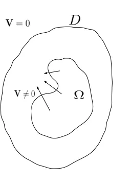
Speed Method
Speed method is a method of constructing continuous domain transformation. Let
Ω⊂Rd be the usual open region of interest. LetT
t be a continuous transformation
on Ω parametrized by a fictitious timet ≥0, i.e. Ωt=Tt(Ω). Equivalently,∀x∈Ω,
xt =Tt(x) at ∀t >0 and T0(x) =x. Furthermore, we let D⊂Rd to be a “holdall”
such that Ωt⊂D for all t >0 and D is not changed by the Tt, i.e.
Tt(D) =D, ∀t ≥0
Such a transformation can be generated by a velocity field V:Rd→
Rd in such
a way that the trajectory of Tt(X),0≤t < for∀X ∈Ω solves the following initial
value problem ([24] Sec.2.9):
d
dtx(t, X) =V(t, x(t, X))
x(0, X) = X
(4.3.1)
Note that if V is smooth enough, then the smoothness of Ω is preserved by the
tranformation generated by B: if Ω is of class Ck and V ∈ Ck(
Figure 4.1: Example of velocity field within a hold-all domain.
of classCk. The notion of admissible velocity field is discussed in [24], Sec.2.9-2.10.
For our purpose, it is sufficient to assume all admissible velocity fields preserve the
smoothness of the original domain Ω for ∀t ∈ [0, ). Note that if V is tangent to
∂Ω, Ω is not changed, i.e. Tt(Ω) = Ω. Following the convention in [24], we use
Vk(D) to denote the space of admissible velocity field.
4.4
Shape Derivative of a Function
In this section, we introduce the notion of material derivative and shape derivative
of a function (cf. [24], Sec2.25, 2.30).
LetW(Ω) be a Banach space of functions defined on the domain Ω and y(Ω)∈
W(Ω). The dependence ofyon Ω is indicated by the bracket on Ω; such dependence
as the solution operator of a boundary value problem. Similarly, we let W(Γ) be a
Banach space on the boundary Γ and z(Γ)∈ W(Γ).
In what follows, we assume a family of domain Ωt is generated by an admissible
velocity field V. Correspondingly, a family of yt(Ωt) and zt(Γt) are generated by
such transformations.
Definition 4.4.1 (Material derivative of a function, [24] Def 2.71). The element
˙
y ∈ W is the material derivative of y(Ω) ∈ W(Ω) in the direction of an admissible
vector field V if the limit exists:
˙
y(Ω;V) = lim
t→0
y(Ωt)◦Tt(V)−y(Ω)
t (4.4.1)
Note the limit can be taken in either the strong sense or the weak sense in W(Ω).
A similar definition exists for z(Γ).
Definition 4.4.2 (Shape derivative of a function of the domain Ω, [24] Def 2.85).
Assume the material derivative ˙y(Ω;V) ∈ W(Ω) and ∇y·V ∈ W(Ω). Then the
shape derivative of y(Ω) in the directionV is the elementy0(Ω;V)∈ W(Ω) defined
by
y0(Ω;V) = ˙y(Ω;V)− ∇y(Ω)·V (4.4.2)
Definition 4.4.3(Shape derivative of a function of the boundary Γ, [24] Def. 2.88).
shape derivative of z(Γ) in the direction V is the element z0(Γ;V)∈ W(Γ) defined
by
z0(Γ;V) = ˙z(Γ;V)− ∇Γz(Γ)·V (4.4.3)
Remark 4.4.4 (Chain rule for shape derivative). From the definition of shape
deriva-tive, it is not hard to see that the chain rule for ordinary derivatives also holds for
the shape derivative. Specifically, if y(Ω) has shape derivative y0(Ω;V) andf(y) is
a smooth function in y, then the shape derivative off[y(Ω)] is simply
f0(Ω;V) = ∂f ∂yy
0
(Ω;V)
Remark 4.4.5. Note the difference in the definition of y0(Ω) and z0(Γ). It is quite
often that z(Γ) is the restriction of a domain function y(Ω) on Γ. In fact, ifz(Γ) =
y(Ω)|Γ, we have the simple but useful identity (cf. [24], Sec. 2.33)
z0(Γ;V) = y0(Ω;V) + ∂y
∂ν hV, νiRd (4.4.4)
where ν is the unit normal vector on Γ.
Remark 4.4.6 (Understandmaterial derivativeandshape derivative). First of all, the
material derivative ˙y(Ω;V) and the shape derivative y0(Ω;V) should be understood
in the sense of directional derivative as defined in Chapter 2. Secondly, ˙y(Ω;V) and
y0(Ω;V) are the analogs of “Lagrangian derivative” and ”Eulerian derivative” in
continuum mechanics, respectively. In some sense, ˙y(Ω;V) is the overal differential
The following example can help understand the difference between material
derivative and shape derivative.
Example 4.4.7. Lety: Ω→Rbe a smooth function on Ω andVbe some admissible velocity field which generates a family of shapes Ωt=Tt(Ω;V). Apparently we have
xt=Tt(x;V) ∀x∈Ω
We define the Ω-dependent function yt to beyt(xt) =y(Tt(x)). Then by the chain
rule, its material derivative in the direction of V is simply
˙
y(Ω;V) =∇y·V (4.4.5)
Let’s consider its shape derivative as a domain functiony(Ω) as well as its restriction
on the boundary y|Γ.
• The shape derivative of y(Ω) is
y0(Ω;V)= ˙d y− ∇y·V= 0 (4.4.6)
From this example, it is easy to see that ˙y reflects the overall rate of change in
yunder the velocity fieldV, whereasy0(Ω) removes the influence of convection
and keeps solely the impact from the change in “shape”.
• The shape derivative of y(Γ) is
y0(Γ;V) = ˙y− ∇Γy·V=
∂y
∂νV·ν (4.4.7)
Thus we see that whenyis viewed as only a function on Γ, its shape derivative
In general, y0(Ω;V) is non-trivial. The map y(Ω) is usually defined by the
solution operator of a boundary value problem on Ω, as we see in the example in
Section 4.7.
Finally, we introduce a lemma from [9] for the computation of the shape
deriva-tive of unit normal vector and mean curvature on a boundary Γ.
Lemma 4.4.8 (Lemma 3.1 in [9]). The shape derivatives of the normal ν and the
mean curvature H of a surface Γ of class C2 with respect to velocity V ∈ C2 are
given by
ν0 =ν0(Γ;V) =−∇ΓV (4.4.8)
H0 =H0(Γ;V) = −∆ΓV (4.4.9)
where V =V·ν is the normal component of the velocity field.
4.5
Shape Derivative of a Functional
Let y(Ω), y0(Ω;V), z(Γ) andz0(Γ;V) be as defined in Section 4.4. In addition, we
let yΓ d
=y(Ω)|Γ to be the boundary value of y(Ω).
Below we present the shape derivative of two special types of functionals:
do-main integrals and boundary integrals. They are applied repeatedly in the shape
sensitivity analysis of our drift-diffusion model in Section 5.3.
the type of integration is indicated by the domain of integration, i.e. Z Ω dV ←→ Z Ω (4.5.1) Z Γ dS ←→ Z Γ (4.5.2)
Such a convention is kept for the remaining of this paper.
• Shape derivative of a domain integral (cf. [24], Sec 2.31)
J1(Ω) =
Z
Ω
y(Ω)
⇒dJ1(Ω;V) =
Z
Ω
y0(Ω;V) + Z
Γ
yV·ν (4.5.3)
• Shape derivative of a boundary integral (cf. [24], Sec 2.33)
J2(Γ) =
Z
Γ
z(Γ)
⇒dJ2(Γ;V) =
Z
Γ
z0(Γ;V) +z HV·ν (4.5.4)
J3(Γ) =
Z
Γ
yΓ =
Z
Γ
y(Ω)|Γ
⇒dJ3(Γ;V) =
Z
Γ
y0(Ω;V) + ∂y ∂νV·ν
+y HV·ν (4.5.5)
Note in equation (4.5.5), we have applied the result of equation (4.4.4).
4.6
The Structure Theorem and Shape Gradient
One of the most important results of shape optimization is the Hadamard-Zol´esio
Structure Theorem. For accurate definition, we refer the readers to [24, 7, 30]. Here
Theorem 4.6.1 (Hadamard-Zol´esio structure theorem). If the shape functional J
is shape differentiable at Ωwith respect toVk(Ω), and Γis sufficiently smooth, then
there exists a scalar Γ-distribution G(Γ) such that
J0(Ω;V) =hG(Γ), γ(V)·νiΓ (4.6.1)
with γ(·) the trace operator on Γ.
What this theorem states is that the sensitivity of a shape differentiable
func-tional only dependes on the normal component of the velocity field. It is certainly
an intuitive result: a velocity field that is tangential to ∂Ω does not change the
shape of Ω, and we do not expect J(Ω) to change if Ω stays the same. In Chapter 5,
we see that the shape sensitivity of photocurrent is supported only on the interface.
Before diving into the shape sensitivity of the photocurrent functional, let’s
compute the shape gradient of some simple examples of geometric quantities.
Example 4.6.2 (Volume of Ω).
J1(Ω) =
Z
Ω
1 (4.6.2)
After taking shape derivative, we have
J10(Ω;V) = Z
∂Ω
1(V·ν) (4.6.3)
Therefore we have obtained the shape gradient of volume: G1 = 1
Example 4.6.3 (Area of∂Ω).
J2(Ω) =
Z
∂Ω
After taking shape derivative, we have
J20(Ω;V) = Z
∂Ω
1·H(V·ν) (4.6.5)
Therefore the shape gradient of surface functional is G2 =H.
As shown above, the computed shape gradients of these simple functionals are
consistent with the structure theorem.
4.7
Example of Shape Optimization
When the functional is associated with some PDE’s, we don’t expect the shape
gradient to take a form as simple as in the last section. To demonstrate the
com-putation for shape gradient, we end this chapter with a simple shape optimization
problem with PDE constraint.
Suppose Ω ⊂ D is a smooth domain in Rd. We only consider the admissible
domains Ω that are contained in some hold-all subset D ⊂ Rd. As we apply the
speed method to find shape sensitivity of a function or a functional, we assume
transformation between admissible domains is generated by some smooth velocity
field V. In what follows, we use V denotes the normal component of V on the
We define the following shape optimization problem with a PDE constraint:
min
Ω J =
Z
Ω
1
2(y−yd)
2
(4.7.1)
where − ∇2y=h Ω (4.7.2)
y= 0 ∂Ω
Here we assume yd ∈H1(D) and h∈L2(Ω) and they are not shape-dependent, i.e.
yd0 =h0 = 0. Note this problem is almost the same example that we presented in
Chapter 2. The only difference is the “control”: here the control is the domain Ω,
or rather the shape of the boundary ∂Ω.
There are two ways to proceed for computing the shape gradient functional.
• One way is to form the nonlinear Lagrangian functional L first, and then
apply shape sensitivity analysis.
• The other way is to compute the shape derivatives of both y and J, i.e. y0
and J0. In particular, we obtain a boundary value problem for y0 which is
linear even if the original PDE is not. The functional J0 is also linear in y0.
Then we form a different Lagrangian functional L based on y0 and compute
the shape gradient.
We show that both methods lead to the same adjoint equations and the same
• Method 1:
Letξ ∈H1(Ω) be the adjoint variable, and thus we have the weak form of the
state equation
Z
Ω
∇y· ∇ξ−
Z ∂Ω ∂y ∂νξ = Z Ω hξ (4.7.3)
Then we form the Lagrangian functional
L= Z
Ω
1
2(y−yd)
2
+ Z
Ω
∇y· ∇ξ−
Z ∂Ω ∂y ∂νξ− Z Ω hξ (4.7.4)
Assume the shape derivative y0 exists. Then we can take shape derivative of
L
L0 = Z
Ω
(y−yd)y0+
Z
∂Ω
1
2(y−yd)
2V
+ Z
Ω
∇y0· ∇ξ+ Z
∂Ω
(∇y· ∇ξ)V
−
Z
∂Ω
h∇y0, νiξ−
Z
∂Ω
h∇y, ν0iξ−
Z ∂Ω ∂ ∂ν ∂y ∂νξ V − Z ∂Ω ∂y ∂νξHV − Z ∂Ω hξV (4.7.5)
where we have applied the formula for computing shape derivative of domain
integral and boundary integral introduced in Section 4.5. We can simplify
this formula further by applying the tangential Green’s formula in Section 4.1
and the shape derivative of outward unit normal vector ν0
L0 = Z
Ω
(y−yd)y0+
Z
Ω
∇y0· ∇ξ−
Z
∂Ω
h∇y0, νiξ
+ Z
∂Ω
1
2(y−yd)
2−∆ Γy ξ−
∂ ∂ν ∂y ∂ν
ξ− ∂y
∂νξH−hξ
If we define the following adjoint equation
− ∇2ξ=−(y−y
d) Ω (4.7.7)
where ξ= 0 ∂Ω (4.7.8)
we have the following integral identities
Z
Ω
(y−yd)y0+
Z
Ω
∇ξ· ∇y0 = Z
∂Ω
y0∂ξ
∂ν (4.7.9)
(4.7.10)
Therefore, we can update L0 as
L0 = Z
∂Ω
y0∂ξ ∂ν +
Z
∂Ω
1
2(y−yd)
2
V (4.7.11)
We have written L0 as a boundary integral. To finally recover the form in the
Structure Theorem, we only need to compute y0 on ∂Ω. In fact, let φ be an
arbitrary smooth function on D
Z ∂Ω yφ 0 = 0 ⇒ Z ∂Ω
y0φ+ ∂y
∂νφV = 0
⇒ y0 =−∂y
∂νV (4.7.12)
Hence we have obtained the shape sensitivity of J
J0(Ω;V) = Z
∂Ω
1
2(y−yd)
2− ∂y
∂ν ∂ξ ∂ν V (4.7.13) (4.7.14)