Material Removal Curve Calculation for
Turbochargers 2 Plane Balancing
Becze Sigismund Vuscan Gheorghe Ioan
Technical University of Cluj-Napoca, Memorandumului 28, 400114 Cluj-Napoca, Romania
Technical University of Cluj-Napoca, Memorandumului 28, 400114 Cluj-Napoca, Romania
Abstract
In the turbocharging business, manufacturers are using industrial balancing machines to balance the so-called center housing rotating assemblies on the production line. The Material Removal Curve calculation is critical for the calibration and prediction of the cut for the turbochargers’ balancing. In practice, the equations resulted from the MRC are used by the software of industrial balancing machines to identify the depth of the cut related to the measured unbalance on the physical CHRA. The software of high-speed turbocharger balancing machines uses, for balancing, calibration parameters resulted from the material removal curve. Those curves are constructed using 3D CAD software matching the unbalance with the depth of the cut (cutting conditions: tool geometry, tool position vs. the part to be cut). The resulted curve is called the Material Removal Curve, which is then approximated with an equation-based curve. The power function curve provides a good approximation, while the 3rd degree polynomial one provides the best match.
Keywords: Turbocharger; Balancing; Material Removal Curve; Calibration; High Speed Balancing Machines
________________________________________________________________________________________________________
I. INTRODUCTION
In the turbocharger industry, the high-speed balancing of the CHRA is critical due to the high rotation service speed. The global influence of the trend for fuel economy had a big impact on the turbocharger business, CHRAs becoming smaller and smaller (the market trend demanding the downsizing of turbochargers), while the rotational service speed increased. In the conditions mentioned above, CHRA high speed balancing became mandatory for all manufacturers in order to ensure a long service life of product. The high-speed balancing machines are complex assemblies of hydraulics, pneumatics, electronics and software which process data and calculate the unbalance [1, 2, 3].
Most (if not all) industrial turbocharger balancing machines use an adequate software for predicting the necessary balancing weight removal and the depth of cut. In order to obtain these values, it is necessary to know in advance some parameters like: tool shape and dimensions, position of the tool vs. the part/component from which the material will be removed, the maximum depth of cut in order to avoid damaging the part or reduce the service life [4, 5]. Those machines are using a CNC axis, so another important factor to know is the tool positioning precision of the axis. Generally, a precision of +/-0.02 mm provides good results. The purpose of this article is to create awareness related to the way of calculating the material removal curve and how those parameters are used [4, 5]. The material removal curve is a curve defined as the correlation between the unbalance and the amount of material removed from a piece. The material removal curve calculation is used to determine the unbalance-depth of cut correlation related to the geometry of different components [6]. This article intends to show the way the material removal curve is determined using a Catia V5 CAD software.
Abbreviations
MRC - material removal curve
CHRA - center housing rotating assembly
CW - compressor wheel
FEA - finite element analysis
II. SIMULATION CONDITIONS
Fig. 1: The compressor wheel milling tool position
Fig. 2: The dimensions of the nut (in mm)
III. CALCULATION AND DATA EVALUATION
CatiaV5 was used for the 3D model simulation and MS Excel for data processing. Considering the first plane on the compressor wheel nut, we have the following steps in the simulation and calculation of unbalance vs. depth: using the CatiaV5 software, the milling tool was positioned at first contact (only touching the nut); the "milling" was done by changing the position up to 2 mm depth with an increment/step of 0.05 mm. After the first “cut”, using a Boolean operation (intersecting the tool with the compressor wheel or nut), the mass of the removed material was measured for every depth and the values were recorded. The results obtained after the last depth of cut are presented in table 1.
Table - 1 Results of the simulation
0.90 0.01003000 13.3480 0.1338805403 0.95 0.01108000 13.3262 0.1476547392 1.00 0.01216000 13.3045 0.1617832064 1.05 0.01329000 13.2829 0.1765298739 1.10 0.01445000 13.2614 0.1916265075 1.15 0.01564000 13.2399 0.2070712540 1.20 0.01687000 13.2184 0.2229949141 1.25 0.01814000 13.1971 0.2393948498 1.30 0.01943000 13.1758 0.2560055997 1.35 0.02075000 13.1546 0.2729581575 1.40 0.02210000 13.1335 0.2902507920 1.45 0.02348000 13.1126 0.3078829088 1.50 0.02488000 13.0917 0.3257222424 2.00 0.04002000 12.8921 0.5159422422
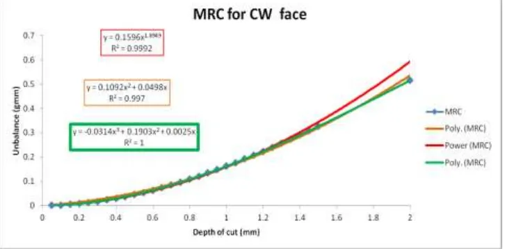
Then, by approximating the curve with a power formula, we obtained an equation. There is a strong link between this equation and the capabilities of the balancing machine’s software algorithm. Most machine balancing software use power functions to predict the depth of cut with only 2 parameters. As can be seen in figure 3, a better approximation can be found using a polynomial function. In the case of compressor face unbalance, a FEA analysis and endurance tests need to be done in order to determine the maximum depth of cut without damaging/reducing the compressor wheel operating life.
Fig. 3 MRC for CW face, where X axis is the depth of cut and Y axis is the unbalance.
The balancing algorithm calculates the unbalance, but needs MRC parameters to predict the appropriate depth of cut for the predicted unbalance. The complexity of the cut depth determination depends on the type of equation used: power or polynomial of 3rd degree. As can be seen from figure 3, the best approximation is obtained when using a 3rd grade polynomial curve, especially for higher unbalances, were the accuracy of the power and 2nd grade polynomial approximations is worse.
The nut MRC setup, that is presented figure 4, was as follows: the tool axis was positioned at 1.5 mm distance from the nut face, at 0 depth on the vertical axis.
The results of the MRC for the nut are presented in table 2.
Table – 2
Results obtained for the nut MRC
Crt no. Depth Mass (g) Radius (mm) Unbalance (gmm) 0.05 0.00010000 4.6371 0.0004637130 0.10 0.00040000 4.6207 0.0018482800 0.15 0.00089000 4.6043 0.0040978092 0.20 0.00157000 4.5879 0.0072029245 0.25 0.00243000 4.5714 0.0111085506 0.30 0.00348000 4.5550 0.0158514000 0.35 0.00471000 4.5386 0.0213766647 0.40 0.00611000 4.5221 0.0276302754 0.45 0.00768000 4.5057 0.0346038528 0.50 0.00942000 4.4893 0.0422889234 0.55 0.01132000 4.4729 0.0506330016 0.60 0.01338000 4.4566 0.0596293080 0.65 0.01559000 4.4405 0.0692269273 0.70 0.01794000 4.4245 0.0793753506 0.75 0.02043000 4.4087 0.0900689238 0.80 0.02305000 4.3930 0.1012574975 0.85 0.02580000 4.3774 0.1129358880 0.90 0.02868000 4.3619 0.1250995788 0.95 0.03167000 4.3466 0.1376565053 1.00 0.03476000 4.3314 0.1505591164 1.05 0.03797000 4.3163 0.1638895313 1.10 0.04127000 4.3013 0.1775134129 1.15 0.04467000 4.2863 0.1914694677 1.20 0.04816000 4.2714 0.2057091792 1.25 0.05174000 4.2565 0.2202292404 1.30 0.05540000 4.2416 0.2349818700 1.35 0.05915000 4.2266 0.2500051645 1.40 0.06297000 4.2117 0.2652094896 1.45 0.06686000 4.1967 0.2805920306 1.50 0.07082000 4.1817 0.2961472858 2.00 0.11338000 4.0276 0.4566470204
The results show that the best approximation is made by the 3rd grade polynomial (green) curve. (Figure 5)
Fig. 5: MRC for CW nut.
IV. CONCLUSIONS
algorithm. The polynomial offers a higher accuracy, but increases the complexity of algorithm which predicts the depth of the cut. One potential way to avoid the algorithm/software complexity could be to create a matching/comparison based on MRC calculation: unbalance vs. depth of cut. This can also increase the amount of manual data input at every new CW or nut, or both, especially if that data is not automatically extracted from the MRC table. The best situation would be to use high precision milling and match the predicted unbalance with the corresponding depth of cut by simple comparison, so the milling axis movement can be correlated with the predicted unbalance. This way, no additional parameters are needed, nor any approximation using coefficients. Of course, ideally speaking, it is possible to obtain a higher accuracy if the tool is measured in advance, if the MRC calculation is adjusted accordingly and if the machine has a high precision in controlling the axes. In some cases, either the tool shape is not the same for both planes (some balancing machines using inserts on a machining bore, while for the CW face a round shape milling tool is used) or the diameter is not the same.
REFERENCES
[1] https://modernpumpingtoday.com/improving-balancing-quality-and-profitability-in-the-overhaul-of-turbochargers/, accessed on 05.03.2019
[2] Mahmoudi A.R., Khazaee I., Ghazikhani M. Simulating the effects of turbocharging on the emission levels of a gasoline engine, Alexandria Eng. J.
2017;56;4;737-48. 10.1016/j.aej.2017.03.005
[3] https://www.melett.com/technicalarticles/chra-balancing-a-critical-part-in-turbocharger-repair/, accessed on 05.03.2019
[4] Calvo J., Diaz V., San Román J. Controlling the turbocharger whistling noise in diesel engines. Int. J. of Vehicle Noise and Vibration. 2, 2006.
10.1504/IJVNV.2006.008524.
[5] Gunter E.J., Humphris R.R., Springer H. Influence of unbalance on the nonlinear dynamical response and stability of flexible rotor-bearing systems, In:
Maurice L.A. editor: Rotor Dynamical Instability. AMD Vol. 55, The applied mechanics, bioengineering and fluids engineering Conference, Huston, Texas, 1983.
[6] Gunter E. J. Unbalance Response and Field Balancing of an 1150-MW Turbine-Generator with Generator Bow, 7th IFToMM-Conference on Rotor