Abstract-- In this study, the theoretical analysis was conducted the three-dimensional turbulent recirculating for air distribution within enclosed cooling space. A modified version of a three-dimensional computer program (fluent 6.3.26) was to simulate the complex flow inside the room by using the Realizable k-ε and SST k-ω models. The study depended on design conditions for Iraq and relying on the Iraqi Code of cooling. The results of numerical model were validate with experimental predications of previous researchers.
The airflow in a room ventilated by displacement diffuser, slot diffuser, square diffuser, and grille diffuser is calculated by the simplified system, respectively. Comparing calculated results to measured data and these comparisons show a good agreement, it is clear that the simplified methodology can predict indoor airflow and temperature gradient with satisfactory results for engineering applications
Index Term-- Numerical simulation, cold air distribution, temperature profile, velocity profile, coanda
I. INTRODUCTION
THAT THE STUDY of the air distribution in enclosed spaces design aspects of the task is to reduce the energy expended to energy consumption and find out suitable climates for people means that a state of thermal comfort has to be achieved on the one hand and the equipment inside spaces on the other hand. Provide the proper climate balance, which concerns people the occupants of a place several values is the speed of the air, the distribution of air temperature, humidity, contaminants, surface temperature of surrounding walls, windows and heating surfaces the ratio of carbon dioxide.
The CDF method of modeling for air diffusers various programs easy way for researchers to knowledge predict the movement of air flow, and all parts must be calculated is included in the internal space to be studied in terms of furniture and appliances.
Many researchers has studied to predict in terms of air diffusers or in terms of the movement of air and temperature
This paragraph of the first footnote will contain the date on which you submitted your paper for review. It will also contain support information, including sponsor and financial support acknowledgment. For example, “This work was supported in part by the U.S. Department of Commerce
under Grant BS123456”.
a: Prof. Sabah Tarik Ahmed, University of Technology, Mechanical Engineering Dept., Iraq, Baghdad ([email protected]). b: Ass. Prof. Ala’a Abbas Mahdi, University of Kufa, Mechanical Engineering Dept., Iraq, An Najaf ([email protected]). b: Eng. Hyder M. Abdul Hussein, University of Kufa, Mechanical Engineering Dept., Iraq, An Najaf ([email protected]).
distribution within the enclosed space and we review them as, “Skovgard and Nielsen (1991), Moser 1991, Zhang et al. 1992, Vogel et al. 1993, Regard et al. 1995, and Jacobsen and Nielsen 1993 Cehlin et al. (2010) modeling the airflow supplied from the diffuser as a major limiting factor in applying CFD to room airflow”,[1,2,3]. and Zhao et al. (2003) used “N-point air supply opening model” is applied to describe boundary conditions of air terminal devices in computational fluid dynamics calculation. They concluded that the box method had better performance, however, this depends on the diffuser-specific data[4]. There are recent studies now theoretical and experimental form of distribution of contaminants as lee et. al. (2009) and Tung et al. (2009) where focused in positive or negative pressure inside the room,[5,6]. Some recently researches as Gharbi et al. (2011) were studied Effect of Different Near-Wall Treatments to obtained a good prediction with the aid of CFD code,[7].
In this work has been to focus on a case study on four types of modeling the most important publisher is (slot (linear) diffuser, displacement diffuser, square ceiling diffuser and grille diffuser) used in the study to the ASHRAE RP-1009 [8] and helpful to measure the results of experimental results measured to be compared with the analysis by CFD, This work was in the modeling of the test chamber to give true behavior with similar indoor furniture and appliances.
II. PHYSICALMODEL
This subject took an experimental air-conditioned room as a simulative object. The size of the room is (5.16 m) long, (3.65 m) wide and (2.43 m) high. In Figure 2 shows how the diffusers were installed in an environmental chamber, The remaining details as dimensions of the Furniture and the dimensions of the diffusers and return taken from the reference [8].
The measuring positions were located at five poles in the chamber (see Figure 1), and vertical distributions of air velocity and temperature were measured,[4]
Fig. 1. Measuring positions in the test chamber,[4].
A Theoretical Study for Cold air Distribution to
Different Supply Patterns
Fig. 2. Positions of the supply diffusers in the room (person - 1, computer - 2, table - III, cabinet - 4, fluorescent lamp - 5, window - 6, exhaust for the
displacement diffuser - 7, exhaust for the mixing diffusers - 8),[8]
III. MAHTEMATICALMODELS
Three-dimensional incompressible turbulence of indoor air by turbulence model was simulated in this paper [9]. To simplify the issue, the models were assumed as follows:
1) The indoor air was incompressible, invariable property, steady-state flow and coincidence with the basic assumption of Boussinesq.
2) Heat-transfer in walls was equable and it was considered as steady-state.
3) Air leakage was without consideration. The door and windows were assumed to be closed when air supplying and their sealing performance was good.
4) Glass scattering to solar radiation and the impact of interior heat-transfer surfaces were considered as constant heat flux.
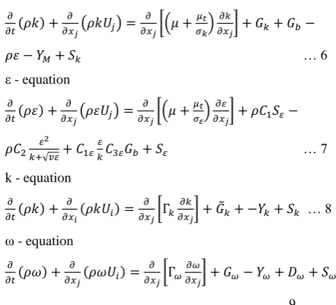
The turbulence model, considering the influence of buoyant force, adopted two-equation Realizable k-ε and k-ω models with the wall-function method.
Continuity equation
( ) ( ) ( ) … 1
X – direction (U momentum)
( ) ( ) ( ) ( ) ( ) ( ) ( ) ( ) ( ) (
) … 2
Y – direction (Y momentum):
( ) ( ) ( ) ( ) ( ) ( ) ( ) ( ) ( ) (
) ( ) … 3
Z – direction (W momentum):
( ) ( ) ( ) ( ) ( ) ( ) ( ) ( ) ( ) (
) … 4 And energy conservation equation
( ) ( ) ( ) ( ) ( ) ( ) (
) … 5
The modeled transport equations for k and ε in the
realizable (k, ε) model are
k - equation
( ) ( ) [( )
]
… 6
ε - equation
( ) ( ) [( )
]
√ … 7
k - equation
( ) ( ) [
] ̃ … 8
ω - equation
( ) ( ) [
]
… 9
Where all constant in equations (6-9) are found in Fluent user's guide,[7].
IV. BOUNDARYCONDITION
At air supply and exhaust the boundary condition for velocity and temperature listed in Table I for validity and Table II for case study at four type of diffuser.
Table I
boundary condition for validity[8].
Diffuser ACH(kg/s) Tsupply Texhaust
Displacement 5.0 (0.0768) 13.0 22.2
Slot (Linear) 9.2 (0.1410) 16.3 21.4
Square Ceiling 4.9 (0.0750) 14.5 24.1
Grille 5.0 (0.0768) 15.1 24.5
Table II
boundary condition for case study.
Diffuser ACH(kg/s) Tsupply Texhaust
Displacement 5.0 (0.0768)
15 24
Slot (Linear) 9.2 (0.1410)
Square Ceiling 4.9 (0.0750)
In addition to the internal heat gains as shown in Table III, there is 341 Btu/h (100 W) to 580 Btu/h (170 W) of cooling load from the window that depends on the diffuser type and ventilation rate
Table III
Internal heat sources in the environmental chamber,[8] Internal Heat Sources Btu/hr (W)
Each human simulator 256 (75)
Computer 1 368 (108)
Computer 2* 590 (173)
Each fluorescent lamp 116 (34)
TOTAL 1935 (567)
* The one close to the window
( ) … 10
… 11
where U0 is the supply velocity, Ti is the turbulence intensity, Cμ= 0.09 is the empirical constant, and l0=0.1L is the length scale. L normally equals to the characteristic length of the diffuser, such as the width of the slot diffuser,[5].
V. NUMERICALCOMPUTATION
The computational meshes were portioned with rectangular coordinate system and describing the mesh model using the Gambit 2.2.30 and the step-size of the main meshes was 0.1m on the directions of three coordinate axes. The meshes were made at human bodies, objects around, air-inlets and air-outlets.
VI. DISCRETIZATIONSCHEMES
The second-order upwind scheme is used for the discretization of the convection terms and the second order. For the discretization of the pressure, the PRESTO! (PREssure STaggering Option) scheme is used. The SIMPLE scheme and SIMPLEC scheme is used for the pressurevelocity coupling[10],[11].
RESULTSANDDISCUSSION
A.EXPERIMENTAL RESULTS
The four test cases are taken from a recent report ASHRAE RP-1009 “Simplified Diffuser Boundary Conditions for Numerical Room Airflow Models” (Chen et al. 2001) [8], indoor conditions imposed in accordance with the design conditions of Iraq depending on The Iraqi Code of Cooling [12] and the results were obtained as we shall. All test cases have the same internal configuration including two human simulators, two computers, two cabinets, two tables (for PC) and four fluorescent lamps. The differences between the test cases are the type and position of the inlet diffuser and the outlet, and the ventilation rate. Curves were classified in the Figures listed below, where reference was made to the experimental given results as (EXP) and the results of the verified (k-ε) and (k-ω) according to the type of model and the results of the case which were held under the design conditions for Iraq (k-ε_c1) and (k-ω), this is underway on all Figures.
B. NUMERICAL RESULTS
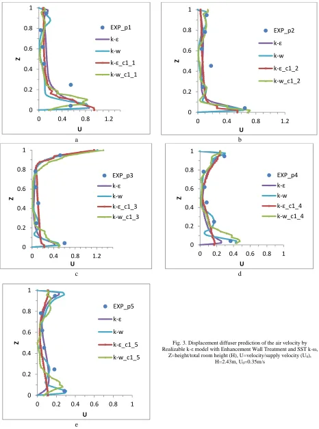
B.1 Displacement Ventilation
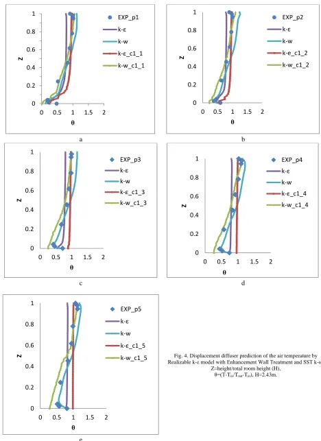
In Figure 3 and 4 a comparison of the predicted air velocity and temperature profiles using Realizable k-ε and SST k-ω model with experiment measurements is given, respectively. The predicted temperatures have some discrepancies with measured data near ceiling and floor, this may be a consequence of the imposed thermal boundary conditions at the ceiling and the floor in the experiment, the measured temperature near the diffuser (17.42°C at X=0.8m) has 3°C difference with the temperature near the West wall and (20.43°C at X=4.36m) has 1.313 °C difference at the floor, by imposing an averaged temperature (23°C) at the floor thus the predicted temperature is lower than the measured value. From Figure 4, it can be seen that the predicted temperatures near the floor are generally lower than the measured ones. Despite the discrepancies, the vertical temperature gradient in the middle of the room is well predicted, which is an important parameter influencing thermal comfort for displacement ventilation.
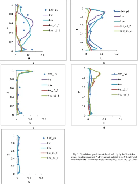
B.2 Ceiling Slot Ventilation
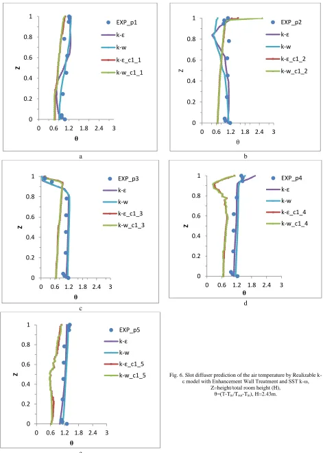
The Figure 5 and 6 gives a comparison of the predicted air velocity and temperature profiles using Realizable k-ε and SST k-ω models with experimental data, respectively. It can be seen that the predicted profiles correspond reasonably well with measured ones. In Figure 5 and 6, the predicted air velocity and temperature profiles at X=1.78m, and 2.51m have some big discrepancies compared with measured data in the ceiling region, this is likely due to the momentum model used for the inlet diffuser, because in Chen et al. 2001 [8] when using the momentum model for the diffuser, they obtained the same results for the predicted temperature profiles, the discrepancies at X=3.36 still exists. When it is used with the k-ε or k-ω models, it may also contribute to some degree to the discrepancies between the predicted temperature profiles and the measured ones. In the occupied zone, thus the prediction using the model for the diffuser is acceptable for practical purposes.
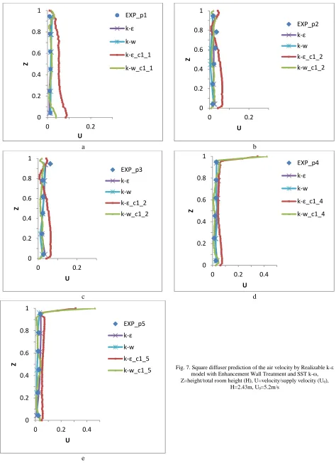
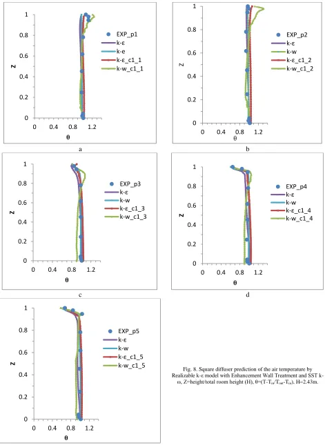
B.3 Ceiling Square Ventilation
Simulations are carried out with the Realizable k-ε, the SST k-ω models and with Box and Momentum methods published. Figure 7 and 8 gives a comparison of the predicted air velocity, temperature profiles using Realizable k-ε and SST k-ω models with experimental data, respectively. It can be seen that the predicted profiles correspond reasonably well with measured ones. In Figure 7, the predicted air velocity profiles at X=0.8m, have some big discrepancies compared with measured data in the ceiling region, and in Figure 8, the predicted air temperature at X=0.8m have some big discrepancies compare with measured date in the floor region, this is due to selected model used for the inlet diffuser, It is noted that the prediction that we have it better than the way from Box and Momentum method.
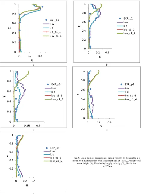
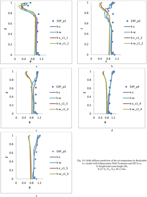
B.4 Grille Ventilation
methods. The results show that the maximum velocity at the jet region in the middle section. However, the calculated
velocity profile presented for pole 1 shows a much higher
maximum jet velocity. In fact, the
measured jet velocity profile in that area is asymmetric due to the possible asymmetric discharge angle. Figure 10 presents calculated and measured temperature profiles. However, the measured jet was closer to the ceiling than the calculated one.
VII. CONCLUSION
In this work simulated cooling for the enclosed room. Numerical analysis based on finite volume method is used to solve three-dimensional steady flow with used k-ε and k-ω turbulent models in resulting temperature distribution and air velocity. The results showed a good comparison with the results of the research [ASHRAE RP-1009] as verify, The results of the case appeared approval for the design conditions placed by the design rules in Iraq in terms of air distribution and temperature distribution. This is something which demonstrates the great potential of the theoretical analysis method used in the search to detect design flaws for air diffusers and locations.
VIII. NOMENCALTURE
u-v-w Velocity component in x-y-z diraction μe The effective viscosity coefficient
ρo The density at reference temperature
Гe, Гk, Гω The effective diffusion
k Kinetic energy
ε Dissipation rate of turbulence energy
ω Turbulence frequency of energy
μt The turbulent or eddy viscosity
Gk, The generation of turbulence kinetic energy due to the mean velocity gradient
Gb The generation of turbulence kinetic
energy due to the buoyancy
Ym The contribution of fluctuation dilution incompressible turbulent
Sε, Sk, Sω, ST
User-define source terms
C1, C2, C3ε, σ3, σk,
Constant
Yk, Yω The dissipation of k & ω due turbulence
Gω The generation of ω
Dω The cross-diffusion term
REFERENCES
[1] Skovgaard, M., and Nielsen, P.V. 1991. Modelling complex inlet geometries in CFD - Applied to air flow in ventilated rooms, Proc. of 12th AIVC Conference, Vol.3, P.P.183-200.
[2] Srebric J. Chen Q. 2002. Simplified Numerical Models for Complex Air Supply Diffusers. HVAC&R Research 8(3) P.P 277-294. [3] M. Cehlin ,B.Moshfegh. 2010, Numerical modeling of a complex
diffuser in a room with displacement ventilation, Building and Environment 45 P.P.2240-2252.
[4] Bin Zhao, Xianting Li, Qisen Yanb Zhao, 2003, A simplified system for indoor airflow simulation. Building and Environment 38. P.P. 543 – 552.
[5] Lee, K.S., Zhang, T., Jiang, Z., and Chen, Q. 2009. Comparison of airflow and contaminant distributions in rooms with traditional displacement ventilation and under-floor air distribution systems, ASHRAE Transactions, 115(2).
[6] Yun-Chun Tung, Yang-Cheng Shih, Shih-Cheng Hu. 2009. Numerical study on the dispersion of airborne contaminants from an isolation room in the case of door opening. Applied Thermal Engineering. 29. P.P. 1544 –1551.
[7] N. El Gharbi, R. Absi, A. Benzaoui, 2011. Effect of Different Near-Wall Treatments on Indoor Airflow Simulations. Journal of Applied Fluid Mechanics, Vol. 4, No. 5, P.P. 63-70.
[8] Chen, Q. and Srebric, J. 2001. Simplified diffuser boundary conditions for numerical room airflow models. Final Report for ASHRAE RP-1009, 181 pages, Department of Architecture, Massachusetts Institute of Technology, Cambridge, MA.
[9] Awbi H. B. 2003. Ventilation of Buildings. Spon Press. [10] FLUENT 6.3 Documentation. 2006. www.Fluent.com .
a b
c d
e
Fig. 3. Displacement diffuser prediction of the air velocity by Realizable k-ε model with Enhancement Wall Treatment and SST k-ω,
Z=height/total room height (H), U=velocity/supply velocity (U0), H=2.43m, U0=0.35m/s
0 0.2 0.4 0.6 0.8 1
0 0.4 0.8 1.2
Z
U
EXP_p1
k-ε
k-w
k-ε_c1_1
k-w_c1_1
0 0.2 0.4 0.6 0.8 1
0 0.4 0.8 1.2
Z
U
EXP_p2
k-ε
k-w
k-ε_c1_2
k-w_c1_2
0 0.2 0.4 0.6 0.8 1
0 0.4 0.8 1.2
Z
U
EXP_p3 k-ε k-w k-ε_c1_3 k-w_c1_3
0 0.2 0.4 0.6 0.8 1
0 0.2 0.4 0.6 0.8 1
Z
U
EXP_p4 k-ε k-w k-ε_c1_4 k-w_c1_4
0 0.2 0.4 0.6 0.8 1
0 0.2 0.4 0.6 0.8 1
Z
U
EXP_p5
k-ε
k-w
k-ε_c1_5
.
a b
c d
e
Fig. 4. Displacement diffuser prediction of the air temperature by Realizable k-ε model with Enhancement Wall Treatment and SST k-ω,
Z=height/total room height (H), θ=(T-Tin/Tout-Tin), H=2.43m. 0
0.2 0.4 0.6 0.8 1
0 0.5 1 1.5 2
Z
θ
EXP_p1
k-ε
k-w
k-ε_c1_1
k-w_c1_1
0 0.2 0.4 0.6 0.8 1
0 0.5 1 1.5 2
Z
θ
EXP_p2
k-ε
k-w
k-e_c1_2
k-w_c1_2
0 0.2 0.4 0.6 0.8 1
0 0.5 1 1.5 2
Z
θ
EXP_p3 k-ε k-w k-ε_c1_3 k-w_c1_3
0 0.2 0.4 0.6 0.8 1
0 0.5 1 1.5 2
Z
θ
EXP_p4
k-ε
k-w k-ε_c1_4
k-w_c1_4
0 0.2 0.4 0.6 0.8 1
0 0.5 1 1.5 2
Z
θ
EXP_p5
k-ε
k-w
k-ε_c1_5
.
a b
c d
e
Fig. 5. Slot diffuser prediction of the air velocity by Realizable k-ε model with Enhancement Wall Treatment and SST k-ω, Z=height/total room height (H), U=velocity/supply velocity (U0), H=2.43m, U0=3.9m/s
.
0 0.2 0.4 0.6 0.8 1
0 0.1 0.2
Z
U
EXP_p1
k-ε
k-w
k-ε_c1_1
k-w_c1_1
0 0.2 0.4 0.6 0.8 1
0 0.1 0.2
Z
U
EXP_p2
k-ε
k-w
k-ε_c1_2
k-w_c1_2
0 0.2 0.4 0.6 0.8 1
0 0.2 0.4
Z
U
EXP_p3
k-ε
k-w
k-ε_c1_3
k-w_c1_3
0 0.2 0.4 0.6 0.8 1
0 0.2 0.4
Z
U
EXP_p4
k-ε
k-w
k-ε_c1_4
k-w_c1_4
0 0.2 0.4 0.6 0.8 1
0 0.2 0.4
Z
U
EXP_p5
k-ε
k-w
k-ε_c1_5
a b
c d
e
Fig. 6. Slot diffuser prediction of the air temperature by Realizable k-ε model with Enhancement Wall Treatment and SST k-ω,
Z=height/total room height (H), θ=(T-Tin/Tout-Tin), H=2.43m.
.
0 0.2 0.4 0.6 0.8 1
0 0.6 1.2 1.8 2.4 3
Z
θ
EXP_p1
k-ε
k-w
k-ε_c1_1
k-w_c1_1
0 0.2 0.4 0.6 0.8 1
0 0.6 1.2 1.8 2.4 3
Z
θ
EXP_p2
k-ε
k-w
k-ε_c1_2
k-w_c1_2
0 0.2 0.4 0.6 0.8 1
0 0.6 1.2 1.8 2.4 3
Z
θ
EXP_p3
k-ε
k-w
k-ε_c1_3
k-w_c1_3
0 0.2 0.4 0.6 0.8 1
0 0.6 1.2 1.8 2.4 3
Z
θ
EXP_p4
k-ε
k-w
k-ε_c1_4
k-w_c1_4
0 0.2 0.4 0.6 0.8 1
0 0.6 1.2 1.8 2.4 3
Z
θ
EXP_p5
k-ε
k-w
k-ε_c1_5
a b
c d
e
Fig. 7. Square diffuser prediction of the air velocity by Realizable k-ε model with Enhancement Wall Treatment and SST k-ω, Z=height/total room height (H), U=velocity/supply velocity (U0),
H=2.43m, U0=5.2m/s
.
0 0.2 0.4 0.6 0.8 1
0 0.2
Z
U
EXP_p1
k-ε
k-w
k-ε_c1_1
k-w_c1_1
0 0.2 0.4 0.6 0.8 1
0 0.2
Z
U
EXP_p2 k-ε k-w k-ε_c1_2 k-w_c1_2
0 0.2 0.4 0.6 0.8 1
0 0.2
Z
U
EXP_p3 k-ε k-w k-ε_c1_2 k-w_c1_2
0 0.2 0.4 0.6 0.8 1
0 0.2 0.4
Z
U
EXP_p4
k-ε
k-w
k-ε_c1_4
k-w_c1_4
0 0.2 0.4 0.6 0.8 1
0 0.2 0.4
Z
U
EXP_p5
k-ε k-w
k-ε_c1_5
a b
c d
e
Fig. 8. Square diffuser prediction of the air temperature by Realizable ε model with Enhancement Wall Treatment and SST
k-ω, Z=height/total room height (H), θ=(T-Tin/Tout-Tin), H=2.43m.
.
0 0.2 0.4 0.6 0.8 1
0 0.4 0.8 1.2
Z
θ
EXP_p1 k-ε k-e k-ε_c1_1 k-w_c1_1
0 0.2 0.4 0.6 0.8 1
0 0.4 0.8 1.2
Z
θ
EXP_p2 k-ε k-w k-ε_c1_2 k-w_c1_2
0 0.2 0.4 0.6 0.8 1
0 0.4 0.8 1.2
Z
θ
EXP_p3 k-ε k-w k-ε_c1_3 k-w_c1_3
0 0.2 0.4 0.6 0.8 1
0 0.4 0.8 1.2
Z
θ
EXP_p4 k-ε k-w k-ε_c1_4 k-w_c1_4
0 0.2 0.4 0.6 0.8 1
0 0.4 0.8 1.2
Z
θ
a b
c d
e
Fig. 9. Grille diffuser prediction of the air velocity by Realizable k-ε model with Enhancement Wall Treatment and SST k-ω, Z=height/total
room height (H), U=velocity/supply velocity (U0), H=2.43m, U0=2.7m/s
. 0
0.2 0.4 0.6 0.8 1
0 0.2 0.4
Z
U
EXP_p1 k-w k-ε k-ε_c1_1 k-w_c1_1
0 0.2 0.4 0.6 0.8 1
0 0.2 0.4
Z
U
EXP_p2 k-w k-ε k-ε_c1_2 k-w_c1_2
0 0.2 0.4 0.6 0.8 1
0 0.2 0.4
Z
U
EXP_p3 k-w k-ε k-ε_c1_3 k-w_c1_3
0 0.2 0.4 0.6 0.8 1
0 0.2 0.4
Z
U
EXP_p4 k-w k-ε k-ε_c1_4 k-w_c1_4
0 0.2 0.4 0.6 0.8 1
0 0.2 0.4
Z
U
a b
c d
e
Fig. 10. Grille diffuser prediction of the air temperature by Realizable k-ε model with Enhancement Wall Treatment and SST k-ω,
Z=height/total room height (H), θ=(T-Tin/Tout-Tin), H=2.43m. 0
0.2 0.4 0.6 0.8 1
0 0.4 0.8 1.2
Z
θ
EXP_p1
k-ε
k-w
k-ε_c1_1
k-w_c1_1
0 0.2 0.4 0.6 0.8 1
0 0.4 0.8 1.2
Z
θ
EXP_p2
k-ε
k-w
k-ε_c1_2
k-w_c1_2
0 0.2 0.4 0.6 0.8 1
0 0.4 0.8 1.2
Z
θ
EXP_p3
k-ε
k-w
k-ε_c1_3
k-w_c1_3
0 0.2 0.4 0.6 0.8 1
0 0.4 0.8 1.2
Z
θ
EXP_p4
k-ε
k-w
k-ε_c1_4
k-w_c1_4
0 0.2 0.4 0.6 0.8 1
0 0.4 0.8 1.2
Z
θ
EXP_p5
k-ε
k-w
k-ε_c1_5
![Table III Internal heat sources in the environmental chamber,[8]](https://thumb-us.123doks.com/thumbv2/123dok_us/1369691.1646789/3.595.48.271.116.291/table-iii-internal-heat-sources-environmental-chamber.webp)