Family income and body mass index

(1)

R E S E A R C H

Open Access

–

what have we learned from China

Fafanyo Asiseh and Jianfeng Yao

*

Abstract

Obesity poses lots of health risks in both developing and developed countries. One thing that remains unclear is the relationship between family income and weight gain. This paper explores the relationship between family income and Body Mass Index (BMI) given variations in individual choice towards basic consumption and life quality improvement consumption as income increases. We use a nationally representative longitudinal data from China, the China Health and Nutrition Survey (CHNS), to estimate the relationship between income and weight gain. We conduct both cross sectional and panel data analysis to study the causal effects of family income on weight development. Unlike other literature that found inverse relationship between prevalence of obesity and family income in developing countries, in this paper, we find that BMI will first increase with family income at a

decreasing rate, and then decrease which suggests that the group of middle class may suffer the high risk of being overweight and obese.

Keywords:Family income, Body mass index, Obesity, Cross section, Panel Data China Health and Nutritional Survey

Background

Obesity poses one of the greatest public health chal-lenges facing both industrialized and developing nations [1]. We see particularly alarming trends in several parts of the world. Policymakers and the public have viewed with concern the dramatic growth in obesity that has taken place in developed countries over the last several decades, and in the recent years, in developing countries as well. In some developing countries, the obesity rate even bypasses the rate in the U.S. and keeps increasing. There is evidence of a strong link between being over-weight or obese and chronic illnesses such as adverse metabolic effects on blood pressure, cholesterol, diabetes and cancer. Obesity also affects workplace productivity [2], employment [3] and the overall demand for and sup-ply of health care [4]. In developing countries, rapid eco-nomic growth has also led to acceleration in nutritional transition in these economies which is contributing to the rate of obesity [5].

In China for example, evidence shows that from 1992 to 2002, there was a remarkable increase in obesity rates among various age groups, regions and gender [6].

Within the same period there was a reported massive growth in China’s economy. From the World Health Organization’s (WHO’s) body mass index (BMI) defini-tion, the rate of overweight and obesity went up from 12.4 to 27.4% from 1991 to 2011 [7]. China was once considered to have one of the leanest populations, but it is fast catching up with the West in terms of the preva-lence of overweight and obesity; disturbingly, this transi-tion has occurred in a remarkably short time. With the economy growing rapidly in China and increasing transi-tion within the populatransi-tion towards more Westernized behavior patterns, diseases related to being overweight are becoming increasingly burdensome and present ur-gent public health challenges, hence preventive strategies are required. Obesity is usually treated as a problem of public health or a misallocation of nutrition. In addition, it can also be regarded as a typical microeconomic prob-lem because, unlike many other diseases, obesity can be avoided through individual behavioral change based on cost-benefit analysis. Naturally, people may rationally prefer to be under or over-weight in a medical sense, be-cause weight results from personal tradeoffs and choices along such dimensions as occupation, leisure-time activ-ity or inactivactiv-ity, residence, and, of course, food intake. Given the variation in their choices about weight, being

* Correspondence:jyao@ncat.edu

College of Business and Economics, North Carolina Agricultural and Technical State University, 1601 E. Market Street, Greensboro, NC 27411, USA

(2)

either fat or thin may be desirable from the individual’s standpoint as adhering to the norms of weight set by doctors and the public health community.

There are a number of reasons for the association be-tween obesity and economic growth in many economies. Finkelstein, Ruhm [8] identified factors such as techno-logical changes that lead to the lower food prices and in-creased food consumption as some of the factors that link economic growth and obesity. These factors also in-creased working hours, which is making more people eat in restaurants and fast food joints. Our study how-ever is based on Blanchard’s model which shows that as wealth increases people may be more likely to spend ini-tially on their material needs. However with time, they may move from just their material needs to healthier choices. This study aims at analyzing the relationship be-tween income and BMI.

The theme of this study is to examine the associations of income with BMI given the variation in individual choices. We further test the hypothesis to investigate the relationship between income and BMI by using the data obtained through a large population based survey con-ducted in both urban and rural areas of regional Main-land China between 1989 and 2011 (CHNS). We analyze the correlation between adult BMI and family income in China looking at both static and dynamic effects. Our estimates are primarily derived using instrumental vari-able and fixed effect regressions, which handle the endo-geneity and heteroendo-geneity issues. We also consider the relationship between income at different intervals, quan-tiles and BMI. Given the structure of the data, the time effects are also taken into accounts.

Our study has a number of key contributions. This study is the first of its kind to analyze the relationship between family income and BMI using a large panel data set from China. Secondly, we explore how income effect varies by gender, age, and different BMI levels. Thirdly, our study investigates how family income and BMI change with time. Our main finding is that there is an inverted U shape between family income and BMI. The probability of being overweight first increases with age and then decreases as people get older. These results are found in both cross sectional and panel data analysis. For example, from a dynamic model, one more year of education increases the BMI by 0.079 units on average. Women’s body mass is roughly 0.491 higher than men’s body mass, and married women on average have a 0.204 lower BMI than single women. Other variables that had an effect on BMI included place of residence, age and education of the respondents.

Literature review

Public health researchers have examined a series of factors in their quest to determine why obesity is

increasing. At the most basic level, obesity is caused by chronic consumption of energy (calories) in excess of energy expended through metabolic and muscular activ-ity [9]. Consequently, more physical activactiv-ity, holding cal-oric intake constant, will result in a decrease in body weight. Studies using individual-level data have also identified race, age, and genetics as factors associated with obesity [10, 11]. Burke and Savage [12] show that the prevalence of obesity is significantly higher among African Americans. Kuczmarski [13] shows that the prevalence of obesity increases with age. Studies of twins have found that genes play a role in determining body mass index [14, 15].

However, a number of researchers have argued the current emphasis on determining the individually based risk factors that are relatively proximate causes of disease (e.g., diet and exercise) tells only part of the story [16–19]. Researchers must also consider the broader social factors that cause exposure to risk factors. Better understanding of how people are exposed to individually based risk fac-tors may permit policy makers to design more effective (or cost-effective) means to combat diseases.

Much of the research on exposure to risk factors uses individual-level data to analyze the link between socio-economic status, typically measured by either income or education, and morbidity or mortality. In the area of obesity, researchers have discovered that the prevalence of obesity is related to income. In a decade of economic growth and rising income, obesity has risen dramatically. This is puzzling when researchers have found that there is inconsistent relationship between income and obesity; most research on overweight and obesity draw on data from industrialized and high income countries, and re-sults have been mixed. In a review of 144 obesity studies, Sobal and Stunkard [20] found that there is a strong in-verse relationship between socioeconomic status (usually defined in terms of education and income) and obesity for women in developed societies the relation for men was weaker. Quintana Domeque and Villar [21] also ex-plored the empirical relationship between family income and BMI in nine European Countries. Their findings suggest that the association is negative for women, but they also found no statistically significant relationship for men. They pointed out that the different relationship for men and women appears to be driven by the negative relationship for women between BMI and individual in-come from work. In support of these findings, Jeffery and French [22] argued that low socioeconomic status subjects lacked access to healthy foods, safe exercise and sound nutritional knowledge that caused their higher rates of obesity.

(3)

prevalence rate of obesity. They employed the micro level data from the 1984–1999 Behavioral Risk Factor Surveillance System. They found a U-shaped effect of BMI on family income and hourly wage rates by age, gender, race, years of formal schooling completed, and marital status. However, their reported coefficients of in-come and inin-come squared are relatively small. Later, Lakdawalla and Philipson [24] presented a dynamic the-ory of body weight and develop its implications. They argued that technological change has induced weight growth by making home- and market-production more sedentary and by lowering food prices through agricul-tural innovation. They also characterized how body weight varies with income. Their study presented de-scriptive empirical evidence that illustrates the inverted U-shaped relationship between body weight and income in U.S. males, suggesting the importance of secular trends in weight gain, which are consistent with the im-pacts of broad-based technological changes. Our study differs from theirs in that we take into account commu-nity- or individual fixed effect to examine the variation of BMI with income over time; i.e., genetic factor in the error term is associated with BMI and other variables such as education, entrepreneurial activity and income [25, 26].

We contribute to the literature studying the relation-ship between income and obesity in the following ways. First, previous researches lack a dynamic framework like what we use to explore the relationship between BMI and family income given variations in individual choices, and this may have significant impact on the results. This study hypothesizes that when income is low, overweight and obesity will start to develop and increase in severity. As income further rises, BMI will continue to increase but at a decreasing rate. Finally, BMI will decrease in in-come and will tend to stabilize (only at this time, they are roughly inversely related). That is why focusing on relatively low income country like China is more likely to let us see the above trend. Secondly, the model might be extended to examine the relationship between income and chronic symptoms like obesity. This dynamic model is inspired by Blanchard [27], but unlike him, we intro-duced a life quality improvement consumption in a closed economy, and our disease (death) rate is not con-stant, where the disease death rate can be determined by the life quality improvement consumption, which is more reasonable. Dynamic analysis and basic consump-tion will further give us a relaconsump-tionship between income and BMI. So, unlike other researchers, our model pre-dicts a roughly inverted U-shaped relationship between BMI, or the prevalence of obesity, and family income. Thirdly, this paper is one of the first studies to use indi-vidual data from a developing country. The earlier litera-ture has studied their association drawing mainly on data from U.S. and other industrialized countries.

Methods Conceptual model

The theoretical framework of relationship between obes-ity and income is inspired by the model of Blanchard [27]. In Blanchard, the model is based on a closed eomy with one final good which has two different con-sumption purposes: one is to satisfy the basic material needs, and two, is to improve the life quality such as dis-ease prevention and body weight control. Within each time period, an individual rationally chooses the fraction of two kinds of consumptions. The finding is that when the income is low, the individual will mostly rely on the first kind of consumption, that is satisfy the basic needs and do not care much about life quality improvement. As a result, investment in disease or obesity control may not be enough. So, this low income individual will tend to gain weight and increase her BMI. As income grad-ually increases, she starts to pay more attention to the life quality improvement, and the investment in body weight control will correspondingly go up. However, achievement of disease prevention and body weight re-duction should be lagged behind. Therefore, as she puts more resources into body weight control, the overweight problem will likely become more remarkable. Only after the treatment reaches a certain level, then body weight will be controlled properly, and with more income and investments, this individual’s BMI will gradually reduce. Later, as the control and treatment costs keep rising, the marginal net benefit of such control will gradually decrease. Thus, after BMI is reduced to certain level, this individual will transfer back the first kind of consumption, and her body weight will tend to stabilize. Therefore, as the income increases, the severity in overweight and obesity will first go up and go down (inverted-U shape).

Theoretical framework

Consider a closed economy composed of an individual and a firm. Individual lives infinitely so that total labor in the economy is Lt= 1 at any time. Within each time

period, the individual offers labor to the firm to let it produce the final good (being combined with capital). This final good has two purposes: one is to provide the basic consumption and two is to improve the quality of life. The individual’s current utility at time

t is u cð Þ ¼t c

1−θ

t

1−θ where ct is the basic consumption and

the parameterθ measures the degree of relative risk aver-sion that is implicit in the utility function (0 <θ <1). On the other hand, if this good is used to build health, it will improve the life quality.

Suppose an individual can always be threatened by dis-eases, we then useptto represent the probability the

in-dividual will get diseases at timet, so, from timet to v, the probability of not getting diseases is exp −R_tvpsds

(4)

Diseases will bring negative effects on individual’s life. When someone is sick, the functionality of her body parts will be affected, and the life satisfaction at current state be discounted. So the larger the possibility of get-ting sick, the lower is the life satisfaction.

Although it is not avoidable that an individual may get diseases in any circumstance, it does not mean that nothing can be done about it. For example, an individual can utilize a part of resource such as the final good men-tioned above to prevent diseases and improve the life quality, which will in turn improve the satisfaction to-wards current life condition. Assume the probability of getting a disease at time t is pt=p(xt), where xt is the

quantity of the final good invested into disease control and life quality improvement. In the initial analysis, we put p xð Þ ¼t ₁_þe1−xθ−σ where σ is exogenous, because after taking the first and second order condition ofp(xt) with

respect to xt, we will get: 1. p' (xt) < 0: as investment of

disease control increases, the probability of getting sick decreases. 2. Whenx<σ,p' ' (xt) < 0: when investment is

small, we won’t see an immediate large effect, and dis-ease probability will slowly decrdis-ease. 3. When x>σ,

p' ' (xt) > 0: after the investment reaches a threshold σ,

the disease precaution will slowly take effect.

From the time period t to infinity, the individual’s ex-pected utility is

EtU¼ Z ∞

t

exp −

Z v

t

psds

⋅e−ρðv−tÞc 1−θ

t

1−θdv ð1Þ

Here, (1) means only in the absence of disease, will an individual completely enjoy her life; when she is sick, she receives no satisfaction during the sick periods. For convenience, we transfer (1) into

EtU¼ Z ∞

t

e−ðpþp xvð ÞÞðv−tÞc 1−θ

t

1−θdv ð2Þ

Whereρð Þxv is the average infection rate between time

t and v, and

ρð Þxv

v−t

ð Þ ¼ Z ∞

t

exp −

Z v

v

p_sds

Assume the capital owned by the individual at time v

is av, and she rents capital to a firm to get interest rvav,

and she also provides the firm with labor to get the wage rate wv. In the meantime, she uses her income for basic

consumption, life quality improvement consumption and capital accumulation:

_

a_v¼rvavþπvþwv−cv−xv ð3Þ

Under this budget constraint, the individual maximizes her expected utility, and we will finally get the

inter-temporal condition of the basic consumption (Euler Equation):

_ c_t ct¼

1

θðrt−ρ−p xð Þt Þ ð4Þ

And from first order conditions, we will also derive the relationship between basic consumption and life quality consumptionxt:

ext−σ

1þext−σ

ð Þ2ct¼1 ð5Þ

We also need to explore the behavior of the firm. Dur-ing each time period, the firm rents capital from the in-dividual and employs labor to produce. Since the individual has invested in life quality improvement and disease control, her productivity will be enhanced. How-ever, this process is unstable and it is hard for a firm to measure it. So, the firm will treat this productivity im-provement as exogenous enhancement and internalize it into the capital and labor:

kα_tx1_t−α−rtkt−δkt−wt ð6Þ

At equilibrium, where at=kt after solving the

maximization problem, the capital accumulation func-tion becomes:

_

k_t ¼kα_tx1_t−α−ct−δkt−xt ð7Þ

Now, from (5), we will easily get the relationship be-tweenctandxt

ct¼ext−σþe−ðxt−σÞþ2 ð8Þ

After taking first order condition of ctwith respect to

xt, we will obtain:

dct

dxt ¼

ext−σ−e−ðxt−σÞ

h i

ð9Þ

Where xt <σ; dc_dxt_t<0; and when xt>σ; dc_dxt_t >0 .

That is to say asxtincreases, the fraction ofctandxtwill

first decrease then increase (U shaped relationship be-tweenctandxtcan be drawn).

Also, we may have the constraint thatct+xt≤f(xt) =yt.

From the above relationship betweenctand xt, we learn

that when the capital stock or output is small, bothctand

xtshould be small, butct/xtis large because when output

is small, even if the individual allocates most resources to the “second” consumption xt, the disease probability

may not be effectively reduced. So, the individual does not care much about the disease at this point and spends most of her income on the“first”consumptionct. After the output level is improved, the individual has the ability to allocate more resources to xt and enough xt

(5)

improvement. So the individual will tend to increase the investment into life quality improvement such as in-crease in household physical activity [28] which will gradually lead to the reduction inct/xt. Finally, when the

production is large enough, a new problem arises; that is the diseasing marginal return of the investment in the disease or obesity control, which means even if thextis

large enough, not much reduction in the disease severity will be observed, that is,ct/xtwill increase again and the

individual weighs more on basic consumption. Such re-lationship between ctand xtcan be used to analyze the

obesity and income level. Suppose the individual’s BMI is determined byct,xt, and other variable vectorht:

∂B cðtð Þyt ;xtð Þyt ;htÞ ∂xt >

0 and ∂B cð tð Þyt ;xtð Þyt ;htÞ

∂xt2 <0 whenct

xt >θ

ctdominatesxt

ð Þ;

∂B cðtð Þyt ;xtð Þyt ;htÞ ∂xt <

0 and ∂B cð tð Þyt ;xtð Þyt ;htÞ

∂xt2 <0 when ct

xt <θ

xtdominatesct

ð Þ;

That is equivalent to: ∂B cðtð Þ;xyt tð Þ;hyt tÞ

∂yt >0, when ct xt>θ;

∂B cðtð Þ;xyt tð Þ;hyt tÞ

∂yt <0, when ct xt <θ.

When income is low, the individual does not care much about the effect brought by the obesity but mainly focuses on the basic consumption; so, as individual’s in-come increases, she will bein-come more and more obese. However, when her income reaches a certain level, the problem of obesity will emerge and become remarkable enough to attract individual’s attention. At this time, the individual also has the ability of controlling this problem by increasing the second consumption. So, the speed of increase in overweight or obesity will gradually slow down. After the investment in obesity control reaches a threshold, say σ’, obesity will be controlled properly and its severity will gradually reduce. Finally, when the in-come is high enough, obesity is under some control, and marginal reduction of BMI or obesity severity is low, people will switch back to consume more ct directly

again, and the individual’s body weight will be stabilized.

Empirical analyses

In our empirical study, we attempt to examine whether, as theoretical analysis predicted, adult BMI is correlated with family income in China, controlling for other fac-tors. We begin with a discussion of several analyses that link income to BMI and obesity. We then specify the empirical test for each analysis.

Cross-sectional framework

Linear regression and quantile regression model

Linear regression is a statistical tool used to model the relation between a set of predictor variables and a re-sponse variable. This model is able to estimate how, on average, family income affects BMI. While this model can address the question“is income important in deter-mining BMI”, it cannot answer the important question “does income influence BMI differently for low BMI than for those who are overweight or obese?”, or put dif-ferently, is the relationship between BMI and income qualitatively equivalent to the relationship between obes-ity and income? A more comprehensive picture of the effect of the predictors on the response variable can be obtained by using quantile regression. Quantile regres-sion models the relation between a set of predictor variables and specific percentiles (or quantiles) of the re-sponse variable. It specifies changes in the quantiles of the response. For example, a median regression of an in-dividual’s BMI on her socioeconomic characteristics spe-cifies the changes in the median BMI as a function of the predictors. The effect of income on median BMI can be compared to its effect on other quantiles of BMI. The quantile regression parameter estimates the change in a specified quantile of the response variable produced by a one unit change in the predictor variable. This allows comparing how some percentiles of the BMI may be more affected by certain individual characteristics than other percentiles. This is reflected in the change in size of the regression coefficient.

Interval regression model

Individual choice towards weight gain and obesity is dif-ferent from normal consumption behavior such as the purchase of goods in the supermarket. The former can be defined as a“long term” behavior, and the results of choice will be revealed after a certain time period, while the latter is the instant choice decision and the choice consequence will be revealed within a short time period. This means that it is improper to use multinomial re-gression model which is used for describing the latter behavior to estimate the former case. The predictor vari-able and response varivari-able of the former lack the clear-cut and immediate decision relationship compared to the latter. Interval regression model estimates an equa-tion on the basis of data in which the dependent variable is only observed to fall in a certain interval or cat-egory on a continuous scale. The data are also cen-sored in the usual sense in that both end intervals are assumed to be open-ended. The latent structure of the model to be considered is assumed to be given by y_i¼x0iβþui (i= 1,…,N), where yi is the

(6)

vectors, the former being repressors and the latter un-known parameters. Theuiare assumed to be independent,

identical and normally distributed random variables with zero mean and varianceσ2 and to be independent of xi.

The conditional distribution of the unobserved dependent variable is given by y_ijxi→N x

0

iβ; σ2

i= 1,…,N. The

ob-served information concerning the dependent variable is that it falls into a certain interval of the real line. The real line is divided into K intervals, the k-th being given by (Ak-1,Ak) and these K intervals exhaust the real line. Thus

A0=− ∞and Ak= +∞, i.e., the first and K-th intervals are

open-ended. The information on the dependent variable is which of these K intervals it falls into, i.e., an indicator vari-ableki(1≤ki≤K) is observed for each i. We will use the

following specification for the interval regression model:

βX ¼β1Yiþβ2Yi2þβ3AGEiþβ4AGEi2

þβ5Diþεi ð10Þ

P BMIð dis¼0jXÞ ¼Fðα1−βXÞ

P BMIð dis¼1jXÞ ¼Fðα2−βXÞ−Fðα1−βXÞ

P BMIð dis¼2jXÞ ¼Fðα3−βXÞ−Fðα2−βXÞ

P BMIð dis¼3jXÞ ¼1−Fðα1−βXÞ

Where α1, α2and α3are thresholds of BMI categories defined by WHO, andDiis a vector of demographic

var-iables including highest education level attained, marital status, urban indicator, gender and region.

Panel data analyses

Using longitudinal data, we will estimate the following specification:

Wit ¼β0þβ1Y eartþβ2Yitþβ3Demogit

þβ4Ageitþβ5Ageit2þεit ð11Þ

The dependent variable is BMI adjusted for reporting error. This variableWplays the same role as in the the-oretical framework. Yitrepresents income, just as in the

theory section, but in this regressionYitwill be included

as a set of dummies indicating the quartile of the income distribution to which an individual belongs. There are two reasons for this. First, this specification allows for the inverted U-shaped relationship we predict. Second, if a person’s actual income is not well calculated or pre-dicted, we can use her income category.Yeartrepresents

a vector of year dummies. Next, we allow for weight to have an inverted U-shape in age: people gain weight as they approach middle age, but they begin to lose weight as they enter old age. This means thatβ4should be posi-tive, while β5 should be negative. Finally, we include a vector of demographic variables, Demogit, that contains

highest education attained, and an indicator for being

married with a spouse presently and an urban indicator. The regression specified above illustrates the conditional variation in weight across groups with different income sta-tus at a point in time (income quartile is always measured in the year of observation, relative to other respondents in that year). By estimating the empirical relationship between weight and various demographic characteristics, we can identify the growth in weight that resulted from demo-graphic changes. The residual change here is attributed to technological change, in the tradition of economic growth-accounting. This relies upon the premise that changes in technology -by altering prices, incomes, and production technologies–cut across the population.

Fixed effect model

Instead of examining variations in income and BMI across individuals at a point in time, we may estimate how changes in individual’s income over time influence changes in BMI over time. Here, if we assume fixed ef-fects, we impose time-invariant individual effects that are possibly correlated with the regressors. Fixed effect model assists in controlling for unobserved heterogen-eity when this heterogenheterogen-eity is constant over time and correlated with independent variables. This constant can be removed from the data through differencing. The model set up is as follows:

BMIit ¼β0þβ1Yitþβ2Demogitþβ3Ageit

þβ4Ageit2þuiþεit ð12Þ

Here, ui is the unobserved individual effect, and εitis

the time-variant error term. ui could represent ability,

genetics or historical factors that do not change over time. In this context,uiis correlated with regressors (i.e.,

unobserved genetics factors are associated with income or demographic variables such as education.), and this unobserved heterogeneity may be purged by using fixed effect regression model.

Formally, we will get:

BMIit−BMIi¼ Xit−XiÞβþ εit−εiÞ

whereXitis a

vec-tor of predicvec-tor variables and X_i¼1

T XT

t¼1Xit is the time average estimator. Therefore, the fixed effect esti-mator is:

^ βFE¼

XI i;t^x

0

itx^it

−1XI

i;tx^

0

it^yit, where ^xit ¼Xit−Xi

and^y_it¼BMIit−BMIi

Results

Data and descriptive statistics

(7)

and Food Hygiene, and the Chinese Academy of Pre-ventive Medicine. The study uses year 2000’s survey data for cross-sectional analysis and nine years’ longitudinal data for panel data analysis (1991, 1993, 1997, 2000, 2004, 2006, 2009 and 2011). The sample households were randomly drawn in eight provinces including Liaoning, Shandong, Jiangsu, Henan, Hubei, Hunan, Guangxi, and Guizhou. Two cities and four counties were sampled in each province. Four neighborhoods in each city, and one county-town in each neighborhood and three villages in each county, were then randomly selected. A neighborhood or village is defined as a com-munity unit. Approximately 20 households were sam-pled per community. The CHNS data contain detailed information on household and individual characteristics as well as health-related information such as physical con-ditions, health behaviors and self-reported health status. The sample was restricted to men and women over the age of 18 for whom there exists a complete set of data on health and demographic variables (age, sex, marital status, education, family income, etc) were available. Since we needed to construct family income, we also exclude those with non-positive family and family income.

We now discuss a variety of measurement issues that need to be clarified before we present the estimation re-sults. The main outcome variable BMI used to measure overweight and obesity, is based on self-reported data on height and weight. This allowed us to define the widely accepted BMI index indicator for each respondent. This index, defined as weight in kilograms divided by the square of height in meters (kg/m2), may also enable us to obtain an estimate of the prevalence of obesity. The WHO (1997) defines BMI below 18.5 kg/m2 as under-weight, BMI of 18.5 to 24.9 kg/m2as normal, BMI of 25 to 29.9 kg/m2as overweight and a BMI of≥30 kg/m2as obese. Observations for those who lost their body parts and who were pregnant since their BMIs are not repre-sentative were also deleted.

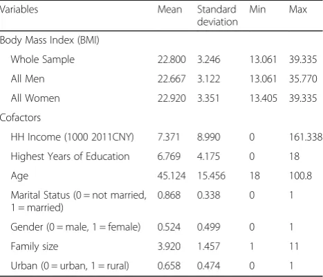
To identify the family income, it is set up as the total household income inflated to 2011. We also control socio-demographic categories including age and age squared, highest education level attained, indicators for sex and marital status, family size, and year, rural and provincial indicators. The descriptive statistics for these variables are shown in Table 1. The average BMI for the population was 22.8, the BMI for women was a little lar-ger (22.9) than that for men (22.6). On average the years of education was 17 years, with the minimum being 0 and the maximum being 22 years. Males made up 53% of the respondents. Majority of the respondents lived in rural areas (65%) and were married (88%). Table 2 pro-vides the descriptive statistics for the panel data. The re-sults are quiet similar to the year 2000 cross sectional data. Tables 8 and 9 in Appendix summarize the

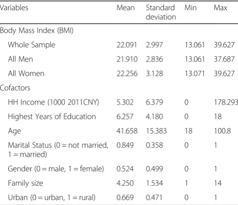
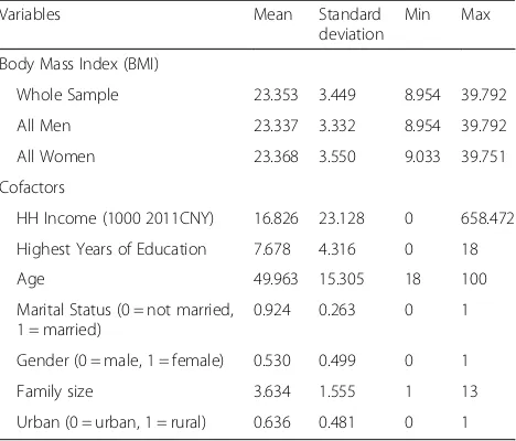
statistics of BMI, family income, and other variables be-fore 2000 and after 2004. We observed positive trends of BMI, income and education, within which income has the fastest growth.

Estimation results

The results for the regression are presented as follows. Table 3 shows the results for the linear regression meas-uring the effect of household income on adult BMI in 2000. To control for the endogeneity problem, family in-come is also instrumented by the family size. Family size is correlated with family income but not associated with error terms such as genetic factors; therefore, it satisfies the conditions for the instrumental variable. The first

Table 1Descriptive statistics of BMI, income and other variables

in China, 2000 (n= 9,506 observations)

Variables Mean Standard deviation

Min Max

Body Mass Index (BMI)

Whole Sample 22.800 3.246 13.061 39.335

All Men 22.667 3.122 13.061 35.770

All Women 22.920 3.351 13.405 39.335

Cofactors

HH Income (1000 2011CNY) 7.371 8.990 0 161.338

Highest Years of Education 6.769 4.175 0 18

Age 45.124 15.456 18 100.8

Marital Status (0 = not married, 1 = married)

0.868 0.338 0 1

Gender (0 = male, 1 = female) 0.524 0.499 0 1

Family size 3.920 1.457 1 11

Urban (0 = urban, 1 = rural) 0.658 0.474 0 1

Table 2Descriptive statistics of BMI, income, and other

variables in China, 1989 - 2011 (n= 80,230 observations)

Min Max

Whole Sample 22.725 3.293 8.954 39.792

All Men 22.622 3.175 8.954 39.792

All Women 22.817 3.393 9.033 39.751

Cofactors

HH Income (1000 2011CNY) 10.642 17.398 0 658.472

Age 45.828 15.896 18 100.8

0.887 0.317 0 1

Family size 3.942 1.575 1 14

(8)

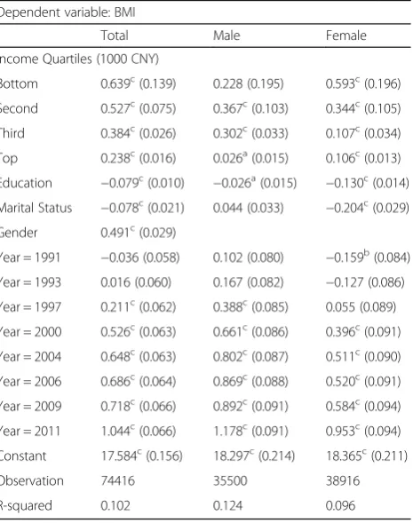
column shows the results for the whole sample, the sec-ond column shows that for men and the third column shows that for women. Table 4 presents results for quan-tile regressions and it shows the effect of family income on different quantiles of BMI. The first column is the 25thpercentile, the second column is the 50thpercentile and the third column is the 75th percentile. In Table 5, we show the results of interval regressions with the ef-fect of family income on various categories of BMI. The first column represents the whole sample the second column represents that for men and the third is that for women. Tables 6 and 7 are both results for the panel re-gressions. Table 6 shows regression results for family in-come on adult BMI between 1991 and 2011 and Table 7 shows the fixed effect model for the regression.

From Table 3, a 1000 CNY increase in family income causes adult BMI to increase by 0.836 units. Men showed a higher increase in BMI (0.856 units) than women (0.640 units). Income squared had a negative effect on the BMI in the whole sample, for both men and women. Once more this effect was more prevalent in men than women. Other confounders also had a significant effect on the adult BMI. We find that age, living in an urban area and being educated all had a significant effect on BMI.

To allow for the possibility of income varying across various BMI levels, a quantile regression was estimated at the 25th, 50thand 75thpercentiles for the whole sam-ple and the results are presented in Table 4. At the 25th

percentile of the BMI, a 1000 CNY increase in family in-come is associated with an increase of 0.809 BMI units. At the 50thpercentile, a 1000 CNY increase in family in-come is associated with an increase of 0.965 BMI units. At the 75thpercentile, a 1000 CNY increase in income is associated with an increase of 0.874 BMI units. Income squared had a negative significant effect on the various BMI levels. This explains the inverted U-shaped rela-tionship between income and BMI. The quantile regres-sion results suggest that the family income has consistent quadratic impact on the different BMI per-centiles. The interval regression results are shown in Table 5, BMI category as defined by WHO is used for

Table 3Linear regressions measuring the effects of family

income on adult BMI, 2000

Dependent Variable: BMI

Whole Sample All Men All Women

Income (1000 CNY) 0.836c(0.094) 0.856c(0.132) 0.640c(0.146)

Income Squared −0.035c(0.008) −0.036c(0.011) −0.030b(0.012)

Constant 16.942c(0.456) 17.590c(0.602) 17.324c(0.632)

Observation 7561 3717 3844

R-squared 0.185 0.181 0.179

Note: Numbers in parentheses are standard errors

b

andc

represent significant level of 10, 5, and 1%

Table 4Quantile Regressions Measuring the Effects of Family

Income on Adult BMI, 2000

Dependent Variable: BMI

0.25 0.50 0.75

Income (1000 CNY) 0.809c_(0.091) _0.965c_(0.136) _0.874c_(0.154)

Income Squared −0.032c(0.007) −0.033c(0.012) −0.033c(0.014)

Constant 15.253c(0.414) 15.854c(0.593) 16.873c(0.681)

Pseudo R-squared 0.046 0.053 0.050

a

,bandcrepresent significant level of 10, 5, and 1%

Table 5Interval regressions measuring the effects of family

income on categorical adult BMI, 2000

Dependent variable: BMI interval

Whole Sample All Men All Women

Income (1000 CNY) 0.522c(0.090) 0.539c(0.125) 0.352b(0.141)

Income Squared −0.024c(0.008) −0.021b(0.010) −0.025b(0.012)

Constant 20.114c(0.435) 20.769c(0.615) 20.701c(0.615)

b

andc

Table 6Regressions of specification (2) measuring the effects of

family income on adult BMI over time, 1991-2011

Dependent variable: BMI

Total Male Female

Income Quartiles (1000 CNY)

Bottom 0.639c(0.139) 0.228 (0.195) 0.593c(0.196)

Second 0.527c(0.075) 0.367c(0.103) 0.344c(0.105)

Third 0.384c(0.026) 0.302c(0.033) 0.107c(0.034)

Top 0.238c(0.016) 0.026a(0.015) 0.106c(0.013)

Education −0.079c_(0.010) ₋_0.026a_(0.015) ₋_0.130c_(0.014)

Marital Status −0.078c_(0.021) _{0.044 (0.033)} ₋_0.204c_(0.029)

Gender 0.491c_(0.029)

Year = 1991 −0.036 (0.058) 0.102 (0.080) −0.159b_(0.084)

Year = 1993 0.016 (0.060) 0.167 (0.082) −0.127 (0.086)

Year = 1997 0.211c_(0.062) _0.388c_(0.085) _{0.055 (0.089)}

Year = 2000 0.526c_(0.063) _0.661c_(0.086) _0.396c_(0.091)

Year = 2004 0.648c_(0.063) _0.802c_(0.087) _0.511c_(0.090)

Year = 2006 0.686c_(0.064) _0.869c_(0.088) _0.520c_(0.091)

Year = 2009 0.718c_(0.066) _0.892c_(0.091) _0.584c_(0.094)

Year = 2011 1.044c(0.066) 1.178c(0.091) 0.953c(0.094)

Constant 17.584c(0.156) 18.297c(0.214) 18.365c(0.211)

Observation 74416 35500 38916

R-squared 0.102 0.124 0.096

a

(9)

analysis. The outputs look very much like the ones from the linear regression model, and the estimation results are similar to those in Tables 3 and 4, which supports the theory that the risk of being overweight or obese, is associated with family income in an inverted U-shaped relationship. We also observed that the impact of in-come on BMI is smaller compared to the quantile and OLS regressions. Similar results were also observed when considering income squared and BMI.

As a means of checking the robustness we included time variables to the estimation. The results for males and females are presented in Table 6, which represents the analysis of BMI variation across different income distributions. We also observe an inverted U-shaped re-lationship for both males and females. We notice that as income level increases, the marginal effects of income on body mass accumulation tends to decrease because of the substitution between the demand for basic consumption and the demand for life quality con-sumption. Table 6, also suggests that weight growth may occur over time. From the coefficients of year dummies, we also observe that males accumulate body mass faster than females. Fixed effect regressions are used to control for the time-invariant heterogeneity and the results are shown in Table 7. Overall, our fixed effect estimators also demonstrate an inverted U-shaped relationship between BMI and household income over time.

Discussion and conclusions

In this paper, we employ micro data from China to pro-vide the theoretical examination and empirical test of the predictions linking household income to adult BMI using both cross-sectional and panel data analysis. We find some evidence supporting our predictions. Our re-sults show an inverted-U shaped relationship between BMI and family income. Additional income brings about higher BMI and higher possibility of being overweight or obese for the poor than for the rich.

Furthermore, from the study, we observe that effect of income on BMI is more prevalent in the OLS regression that the other estimates that were done. Additionally, we find that relationship between income and BMI was more prevalent among those in the 50thincome percen-tiles. The BMI of males were more affected by family in-come than for women. Incorporating panel data in our study, we find that the relationship between BMI and in-come has been increasing over the years in China. In-creased levels of BMI in general are troubling since this will also lead to an increase in chronic diseases among the population. Based on the cofactors we also find that the BMI increase was greatest in middle ages. This is very serious especially given the fact that middle age population plays a significant role in the growth and de-velopment of the economy.

While this study has its own limitations, it is among the first to provide evidence from a developing country on the nonlinear relationship between family income and BMI. Although the sample size is relatively small compared with the data in many U.S. studies, the set of CHNS data we have used is so far one of the best data sets used in studying income and BMI in the context of developing economies, and is probably the best Chinese data set. Finally, strictly speaking, our empirical tests are tests of correlations between family income and individ-ual BMI. The causal link may not be established until more evidence becomes available regarding the inter-mediate mechanisms through which income affects obesity. However, we do find there is a strong relation-ship between family income and BMI.

Appendix

Table 7Individual fixed effect regressions measuring the effects

of family income on adult BMI over time, 1991–2011

Dependent variable: BMI

Total All Male Female

Income Quartiles (1000 CNY)

Bottom 0.459c(0.082) 0.734c(0.117) 0.254b(0.114)

Second 0.219c(0.043) 0.137b(0.060) 0.263c(0.059)

Third 0.035b(0.017) 0.038b(0.021) −0.005 (0.020)

Top 0.021a(0.011) −0.020b(0.010) 0.025c(0.009)

Constant 14.052c(0.118) 13.619c(0.161) 14.600c(0.176)

Observation 74416 35500 38916

a

,b

andc

Table 8Descriptive statistics of bmi, income, and other

variables in China, 1989–2000 (n= 39,952 observations)

Min Max

Whole Sample 22.091 2.997 13.061 39.627

All Men 21.910 2.836 13.061 37.687

All Women 22.256 3.128 13.071 39.627

Cofactors

HH Income (1000 2011CNY) 5.302 6.379 0 178.293

Age 41.658 15.383 18 100.8

0.849 0.358 0 1

Family size 4.250 1.534 1 14

(10)

Authors’contribution

FA was responsible for the introduction, literature review section. JY was responsible for model development, theoretical and empirical analysis. Both authors worked on approving the model, interpreting results and discussion. Both authors read through and approved every aspect of the paper.

Competing interests

The authors declare that they have no competing interests.

Received: 9 June 2016 Accepted: 24 October 2016

References

1. Au N, Johnston DW. Too much of a good thing? Exploring the impact of wealth on weight. Health Econ. 2015;24(11):1403–21.

2. Ketter P. Obesity affects workplace productivity. T+ D. 2006. p. 60. 3. Kristen E. Addressing the problem of weight discrimination in employment.

California Law Review. 2002;90(1):57–109.

4. Finkelstein EA, Strombotne KL. The economics of obesity. Am J Clin Nutr. 2010;91(5):1520S_–4.

5. Popkin BM, Adair LS, Ng SW. Global nutrition transition and the pandemic of obesity in developing countries. Nutr Rev. 2012;70(1):3–21.

6. Wang Y, et al. Is China facing an obesity epidemic and the consequences? The trends in obesity and chronic disease in China. Int J Obes. 2007;31(1):177–88.

7. Institute for Health Metrics and Evaluation. Overweight and Obesity VIZ. 2014 6/3/2016]; Available from: http://vizhub.healthdata.org/obesity/. Accessed 14 Nov 2016.

8. Finkelstein EA, Ruhm CJ, Kosa KM. Economic causes and consequences of obesity. Annu Rev Public Health. 2005;26:239–57.

9. Nestle M, Jacobson MF. Halting the obesity epidemic: a public health policy approach. Public Health Rep. 2000;115(1):12.

10. Tremblay A, Doucet E, Imbeault P. Physical activity and weight maintenance. Int J Obes. 1999;23:S50–4.

11. Bouchard C, Perusse L. Genetic aspects of obesitya. Ann N Y Acad Sci. 1993;699(1):26_–35.

12. Burke GL, et al. Correlates of obesity in young black and white women: the CARDIA Study. Am J Public Health. 1992;82(12):1621–5.

13. Kuczmarski RJ. Prevalence of overweight and weight gain in the United States. Am J Clin Nutr. 1992;55(2):495S_–502.

14. Stunkard AJ, et al. Weight change in depression: influence of

“disinhibition”is mediated by body mass and other variables. Psychiatry Res. 1991;38(2):197–200.

15. Price RA, et al. Genetic contributions to human fatness: an adoption study. Am J Psychiatry. 1987;144(8):1003–8.

16. Krieger N. Epidemiology and the web of causation: has anyone seen the spider? Soc Sci Med. 1994;39(7):887_–903.

17. Link BG, Phelan J. Social conditions as fundamental causes of disease. J Health Soc Behav. 1995;80–94 (extra issue).

18. Link BG, Phelan JC. McKeown and the idea that social conditions are fundamental causes of disease. Am J Public Health. 2002;92(5):730_–2. 19. McKinlay JB, Marceau LD. A tale of 3 tails. Am J Public Health. 1999;89(3):295–8. 20. Sobal J, Stunkard AJ. Socioeconomic status and obesity: a review of the

literature. Psychol Bull. 1989;105(2):260.

21. Quintana Domeque, C. and G. Villar, Income and body mass index in europe. Department of Economics and Business, Universitat Pompeu Fabra series Economics Working Papers, 2008(1001).

22. Jeffery RW, French SA. Socioeconomic status and weight control practices among 20-to 45-year-old women. Am J Public Health. 1996;86(7):1005_–10. 23. Chou S-Y, Grossman M, Saffer H. An economic analysis of adult obesity:

results from the behavioral risk factor surveillance system. J Health Econ. 2004;23(3):565–87.

24. Lakdawalla D, Philipson T. The growth of obesity and technological change. Econ Human Biol. 2009;7(3):283–93.

25. Silventoinen K, et al. Trends in obesity and energy supply in the WHO MONICA Project. Int J Obes. 2004;28(5):710–8.

26. Nicolaou N, et al. Is the tendency to engage in entrepreneurship genetic? Manag Sci. 2008;54(1):167–79.

27. Blanchard, O. J.. Debt, Deficits and Finite Horizons. National Bureau of Economic Research Working Paper Series, 1984. No. 1389.

28. Ford ES, et al. Physical activity behaviors in lower and higher socioeconomic status populations. Am J Epidemiol. 1991;133(12):1246–56.

Submit your manuscript to a

journal and beneﬁ t from:

7Convenient online submission 7Rigorous peer review

7Immediate publication on acceptance 7Open access: articles freely available online 7High visibility within the ﬁ eld

7Retaining the copyright to your article

Submit your next manuscript at 7 springeropen.com

Table 9Descriptive Statistics of BMI, Income, and Other

Variables in China, 2004–2011 (n= 40,278 observations)

Min Max

Whole Sample 23.353 3.449 8.954 39.792

All Men 23.337 3.332 8.954 39.792

All Women 23.368 3.550 9.033 39.751

Cofactors

HH Income (1000 2011CNY) 16.826 23.128 0 658.472

Age 49.963 15.305 18 100

0.924 0.263 0 1

Family size 3.634 1.555 1 13