Nat. Hazards Earth Syst. Sci., 10, 1051–1059, 2010 www.nat-hazards-earth-syst-sci.net/10/1051/2010/ doi:10.5194/nhess-10-1051-2010
© Author(s) 2010. CC Attribution 3.0 License.
Natural Hazards
and Earth
System Sciences
An expression for the water-sediment moving layer in unsteady
flows valid for open channels and embankments
A. M. Berta and G. Bianco
Dipartimento di Idraulica Trasposti ed Infrastrutture Civili, Politecnico di Torino, Torino, Italy
Received: 5 October 2009 – Revised: 5 February 2010 – Accepted: 23 February 2010 – Published: 28 May 2010
Abstract. During the floods, the effects of sediment trans-port in river beds are particulary significant and can be stud-ied through the evolution of the water-sediment layer which moves in the lower part of a flow, named “moving layer”. Moving layer variations along rivers lead to depositions and erosions and are typically unsteady, but are often tackled with expressions developed for steady (equilibrium) condi-tions. In this paper, we develop an expression for the mov-ing layer in unsteady conditions and calibrate it with ex-perimental data. During laboratory tests, we have in fact reproduced a rapidly changing unsteady flow by the ero-sion of a granular steep slope. Results have shown a clear tendency of the moving layer, for fixed discharges, toward equilibrium conditions. Knowing the equilibrium achieve-ment has presented many difficulties, being influenced by the choice of the equilibrium expression and moreover by the es-timation of the parameters involved (for example friction an-gle). Since we used only data relevant to hyper-concentrated mono-dimensional flows for the calibration – occurring for slope gradients in the range 0.03–0.20 – our model can be ap-plied both on open channels and on embankments/dams, pro-viding that the flows can be modelled as mono-dimensional, and that slopes and applied shear stress levels fall within the considered ranges.
1 Introduction
Sediment transport effects are particulary significant during the floods and their study is important for a better under-standing of hydrodynamical and morphological processes. A useful indicator of the sediment discharge is the depth of the water-sediment layer which moves in the lower part of a stream, named “moving layer” or “bed load layer” (Egashira and Ashida, 1992). If related to the flow depth (measured
from the granular layer that is not in motion), the moving layer is commonly used to distinguish the different kinds of flow (ordinary flow, hyper-concentrated flow). For example, ordinary flows present a ratio far less than unity between the width of the moving layer and the depth of the water-sediment flow. Hyper-concentrated flows are instead char-acterised by a moving layer comparable to flow depth, and so not negligible. A correct evaluation of the moving layer is particularly important when the sediment transport is intense, because mistakes may have many consequences on the water level estimation.
Transport processes in alluvial channels are usually un-steady and produce spatial and temporal changes of river morphology that can be related to the continuous variation of moving layer thickness. Unfortunately, there are only few works regarding the unsteady non-uniform sediment trans-port, and unsteady flows are usually treated with expressions that have been developed for a uniform flow condition (Papa et al., 2004; Egashira et al., 2001; Franzi, 2001; Correira et al., 1992; Takahashi, 1991) that is often described as the “equilibrium condition” (Seminara, 1998). This approach is incorrect for purely unsteady flows, for which the immedi-ate achievement of transport capacity, which actually occurs in equilibrium conditions, is not ensured (Armanini and Di Silvio, 1988). The immediate achievement of transport ca-pacity can be admitted, usually for granular materials, when time dependent effects are negligible. This approximation is not reliable for strictly unsteady flow (with a strong de-pendence on time) and with little erosion length available. In fact, in some of their tests carried out with constant liquid discharge, Di Silvio and Gregoretti (1997) doubted that equi-librium conditions were effectively reached as a consequence of a too short erodible flume.
labo-1052 A. M. Berta and G. Bianco: An expression for the weater-sediment moving layer in unsteady flows
1
An expression for the water sediment moving layer in
unsteady flows valid for open channels and embankments
A. M. Berta
1and G. Bianco
1[1]{Dipartimento di Idraulica Trasposti ed Infrastrutture Civili, Politecnico di Torino, Torino,
Italy}
Correspondence to: A. M. Berta (anna.berta@polito.it)
Figure 1. Sketch of the moving layer depth
h
sof a flow over an erodible bed. Profiles for
velocity
u(z)
and sediment concentration
c(z)
(Egashira and Ashida, 1992).
Fig. 1. Sketch of the moving layer depthhsof a flow over anerodi-ble bed. Profiles for velocityu(z)and sediment concentrationc(z) (Egashira and Ashida, 1992).
2
0,0 0,5 1,0 1,5 2,0 2,5 3,0
0 2 4 6 8 10 12 14 16
Θ/Θcr hs
/d
eq.Takahashi (1991)
eq.Egashira (1992) eq.Berta (2008) eq.Franzi (2001)
tan ϑ = 10%
Φ = 55° d = 1,55 mm
Figure 2. Non-dimensional moving layer depth,
h
s/d
, against
Θ/Θ
cr,
estimated with different
expressions developed for steady flows. Values of slope, friction angle and diameter used for
the estimation are shown in the figure.
Fig. 2. Non-dimensional moving layer depth,hs/d, against2/2cr,
estimated with different expressions developed for steady flows. Values of slope, friction angle and diameter used for the estimation are shown in the figure.
and Bowles, 2006), we have reproduced a rapidly changing unsteady flow through the overtopping of a granular steep slope. To make our model comparable with the ones de-veloped for open channels, only data relevant to the mono-dimensional erosion stage have been used for the calibration. Consequently, our model can be applied both to open chan-nels and to embankments/dams, provided that the flows can be modelled as mono-dimensional and that the slopes and shear stress levels fall within the considered ranges.
2 Evaluation of moving layer depth in unsteady flow
It is observed that, during an erosive process, the moving layer depth,hs (see Fig. 1), increases from zero (if the
in-coming stream is clear water) to a maximum value, when the transport capacity is completely satisfied (Egashira and Ashida, 1992). Many formulas for hs have been
devel-oped for uniform flow condition, or “equilibrium condition”, where the transport capacity is satisfied. For example, in Fig. 2 are represented Egashira and Ashida (1992),
Taka-3
Figure 3. Sketch of the sediment transport scheme.
Fig. 3. Sketch of the sediment transport scheme.
hashi (1991), Franzi (2001) and Berta (2008) expressions for the non-dimensional moving layer,hs/d(dis the
representa-tive diameter). The curves in Fig. 2 show the trend of increas-inghs with2/2cr(where2cris the critical Shields
param-eter), and describes only the equilibrium value ofhs, so this
cannot describe the evolution of the moving layer. Hence, our purpose is to describe the evolution of the moving layer for generic unsteady conditions.
We adopt a phenomenological scheme that was first pro-posed by Du Boys (Wan and Wang, 1994), then resumed by Chien and Wan (1999), Bianco and Franzi (1999), and Franzi (2001). Even though developed for steady conditions, this approach here is supposed to be valid also in unsteady conditions, by assuming all the variables varying in space and time. Our scheme considers an infinitely long bed of in-coherent particles, with slopeϑ. The motion of each layer is assumed to be mono-dimensional and is thought to be due to two effects: the component of weight force parallel to the flow direction (x, see Fig. 3) and the drag of the flow, and the resistance to motion is due instead to the friction acting between the particles in the considered layer and those be-low it. Equilibrium equation for thex direction in uniform conditions can be written as follows:
ρw
2 (u0−u1)
25α2d2
4 +(ρs−ρw) 5
6α
3d3sinϑ=
K1g (ρs−ρw)
5 6α
3d3cosϑ (1)
where u0 is the flow velocity (defined in a time interval
smaller than the time scale of the unsteadiness) over the first grain layer;u1is the velocity of the first layer;K1is a
dimen-sionless coefficient which takes into account the frictional ef-fects due to interaction between water and sediment;gis the acceleration due to gravity,ρsandρware sediment and water
density, respectively;αis a coefficient related to the particles
A. M. Berta and G. Bianco: An expression for the weater-sediment moving layer in unsteady flows 1053 distance (which can be less or more than diameterd) and
supposed to assume the form: α=β
rτ 0
τc
, (2)
whereβ, unknown, is a calibration parameter,τ0the bottom
shear stress andτcits critical value. After simplifications, the
equation system which describes each layer motion is:
(u0−u1)2=43
ρs
ρw−1
αgd (K1cosϑ−sinϑ )
(u1−u2)2=43 ρ
s
ρw−1
αgd (2K2cosϑ−sinϑ ),...,
(un−1−un)2=43
ρ s
ρw−1
αgd (nK2cosϑ−sinϑ )
(3)
where coefficientK2takes into account the effects of the
su-perior moving layers and the resistance effect of the lower ones. Following Takahashi (1991),K2is assumed:
K2= c∗
Cv 13
tan8, (4)
whereCvis the average concentration of the water sediment
flow andc∗is the mean dry volumetric concentration of the bottom. Dividing each equation by(∂y)2∼=(αd)2, the equa-tion system can be rewritten in a differential form:
∂u
∂y
2
=4
3(K2ycosϑ−αdsinϑ ) g
ρ s
ρw
−1
1
(αd)2 (5) Equation (5) is integrated in space (boundary condition: u(0)=u1), and divided by the friction velocity, u∗. The
moving layer depth,hs, is established by imposingu(hs)=0.
hs d = 3 2 ˜ N β
232
K2∗
13 s2
2c
−1
!23
(6) In Equation (6), 2c is the critical Shields parameter
(cor-rected for slope);2is the Shields parameter and is estimated for unsteady flows with the energy slope,Se, instead of the
bottom slope (Graf and Song, 1995): 2= τ0
(γs−γ )d
= R Se
ρs
ρ −1
d
; (7)
˜
N is the approximation of expressionu0/u∗ for critical
in-cipient motion condition; and
K2∗=4/3(K2cosϑ−sinϑ ) . (8)
The function32N β˜ 2
/3is supposed to depend on hydrody-namical conditions,2c/2, and on sediment diameter,d. Our
model is consequently written as: hs
d =F
2 c
2,d 2 K2∗
1/3 s2
2c
−1
!2/3
. (9)
3 Experimental Setup
3.1 Hydraulic setup
Laboratory experiments were conducted in a 20 m long, 0.395 m wide straight flume with plexiglass walls and a slope equal to if =0.00715. A 0.395 m wide trapezoidal wooden template, composed of several modules, was located at the end of the flume (Fig. 4). The embankment was made erodi-ble over a width of 0.095 m next to the left side of the flume by substituting one of the fixed modules with granular mate-rial. The sediment was thoroughly mixed by hand and shaped like a wooden dam (Fig. 4). A 0.03 m thick and 0.70 m long drain was placed under the embankment to prevent fail-ure during the filling of the flume. The water level in the flume was raised to the level of the embankment crest (about 0.13 m); when water started to flow over the structure, the canal was no longer fed and the breaching process sponta-neously evolved. The canal freely emptied at a rate that was dependent on the erosion development. A metal plate sep-tum, placed behind the embankment, narrowed the width of the flume to 0.095 m and ensured a regular and parallel flow. Water discharge,Qw, which flew over the embankment, was
estimated through the variations in time of water volume in the flume, detected by a level probe. Adopting the exper-imental techniques used by Visser (1998) and Coleman et al. (2002), the water levels were measured (at 10 Hz) by the probe which was positioned upstream to the structure. As the overtopping discharge progressively eroded the embank-ment, a hopper at the end of the flume collected water and the sediment output. A sediment trap was placed under the hopper: the trap base, made of a mesh filter, was linked to a loading cell which recorded the dynamic force of the water-sediments (frequency 10 Hz). Data processing allowed the sediment discharge,Qs, to be estimated. The erosion
pro-cess was videotaped from downstream with a digital video camera and photographed with a digital camera (respectively VC1 and DC1 in Fig. 3) placed on one side of the flume. The profiles and local slopes of the free stream surface and of the embankment were recognized from each frame. Moving layer measures,hs, were acquired along inner sections over
the slopes.
3.2 Sediment properties
In order to analyse the influence of the sediment mean di-ameter on the moving layer depth, three different sediments (named A, B and C) were used to build erodible embank-ments. Some of their key properties are shown in Table 1.
4
Figure 4. Sketch of the flume in the experiment. Water flows from right to left.
Fig. 4. Sketch of the flume in the experiment. Water flows from right to left.
Table 1. Properties of sediments and embankments: for the three
sediments (indicated as A, B, C) are shown the different granulom-etry, the mean diameter,d50, and the specific gravityGs. For the
different embankments are collected the mean dry volumetric con-centrations,c∗.
Sediment and A (test 31) B (test 28) C (test 26) reference test
Granulometry 0.1-0.71 1.41–1.68 50%(1.41–1.68) (mm) 50%(0.35–0.5) d50(mm) 0.86 1.55 0.99
Gs 2.649 2.663 2.656
c∗ 0.565 0.620 0.631
Table 2. Constant volume8cv(measured using a tilting table
cov-ered by fixed grains of the same size) and peak friction angle8p
(measured for specimens with relative density DR=25). Sediment A B C 8cv(◦) 37.3 39.1 38.7
8p(◦) 53.4 55.9 55.0
relative density, DR, affects friction angle,8. It should be pointed out that what is commonly identified as friction an-gle is in fact the peak friction anan-gle,8p, which assumes a
lower value for sediment in a loose state (8cv: constant
vo-lume friction angle) and increases, due to a dilatancy
phe-Table 3. Description and average peak friction angle8p
(represen-tative of the three materials A, B, C) for the embankment layers, identified through the downstream embankment slopes tanϑ.
Layers Range of slopes Average8p
surface 0.33 39◦ 1 0.33<tanϑ <0.25 43◦ 2 0.25≤tanϑ <0.17 47◦ 3 0.17≤tanϑ <0.09 51◦ 4 0.09≤tanϑ≤0 55◦
nomenon, with the relative density, DR (Bolton, 1998). Ac-cording to Bolton’s theory, we have experimentally enhanced the friction angle through a particular building technique. As the embankment was built layer by layer, the most internal region was more compacted than the external one, while the sediment in the upper layer could be considered in a loose state. During our tests, water overflowed the embankment and the erosion, in time, affected the layers with increased compactness: for the sake of simplicity, we have considered the structure to be divided into five zones with homogeneous compaction (and, hence, relative density DR) (Fig. 5). Tests on specimens for each sediment composition were performed in order to assign reliable peak and constant volume friction angle value to each embankment zone (Table 2). An average friction angle, representative of the three sediments, was as-signed to each compaction zone: the maximum peak friction value (55◦) assigned to the bottom layer, was decreased to the critical value (39◦) for the upper one (Table 3).
A. M. Berta and G. Bianco: An expression for the weater-sediment moving layer in unsteady flows 1055
Figure 5. Cross section of the embankment with the hypothesis of five homogenous
compactness zones (identified as surface, 1, 2..4). The erosion, in time, affected layers with
increasing compactness: at first, the upper layer (surface and nr.1) and afterwards the lower
layers (nr. 2-3). Flume water is on the right side of the section.
Fig. 5. Cross-section of the embankment with the hypothesis of
five homogenous compactness zones (identified as surface, 1, 2...4). The erosion, in time, affected layers with increasing compactness: at first, the upper layer (surface and nr. 1) and afterwards the lower layers (nr. 2–3). Flume water is on the right side of the section.
4 Results
The erosion of the embankment reproduced a continuous evolution of streams from debris flows to ordinary bed loads. A distinction of the different stages of erosion is useful to un-derline the occurrence of a stage (the third) in which the wa-ter sediment stream was approximately mono-dimensional. The data acquired during this stage were considered compa-rable to open channel data, and were used to calibrate Eq. (9). 4.1 Erosion stages of embankment
As the overflowing began, four stages were observed, with the consequent erosion.
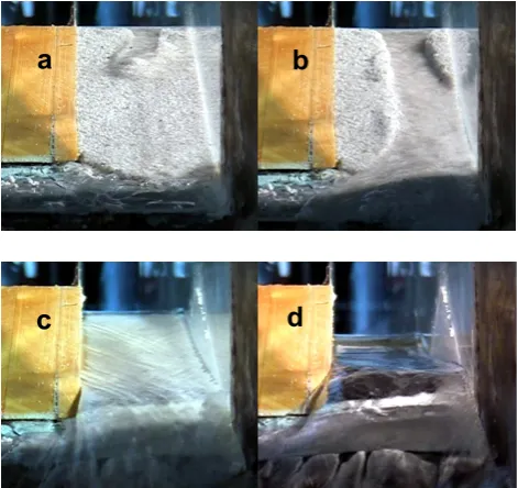
In the first stage (Fig. 6a), the opening of one or more breaches was recognized. Crest particles, in a loose state, were easily moved by the initial overflowing discharge: as a result, a sliding of sediment particles occurred and a small debris flow started. In the second stage (Fig. 6b), the erosion of the slope continued in small channels and progressively expanded laterally to cover the whole slope width. The in-creased scour led to an inin-creased water discharge, with a sig-nificant unsteadiness. The third stage (Fig. 6c) began when the stream occupied the whole slope width and the erosive phenomenon affected only the embankment bed, and pro-gressively reduced its slope. From the beginning of this phase until the complete embankment erosion, the stream ap-peared dominated by the longitudinal velocity component, in a process that could be regarded as well approximated by a one-dimensional flow model. In the fourth and last stage (Fig. 6d), the flume emptied: this stage began at the complete erosion of the structure, when the water was able to occupy the whole transverse section.
4.2 Water, sediment discharges and sediment concentration
The overflowing water discharge,Qw, is computed by
sub-tracting the seepage discharge from the total discharge flow-ing out of the flume, dV/dt (variation in timet of the
wa-Fig. 6 Downstream view of the embankment erosion.
a)
Stage 1: water reaches the
embankment crest, particles are easily moved and a little debris flow originate;
b)
Stage 2:
erosion of the slopes, started in small rills, continues within small channels progressively
widening to the whole width. Increasing scour lead increasing water discharge, so debris flow
evolves into immature debris flow;
c)
Stage 3: water sediment stream, occupying all the
embankment width, is approximately mono-dimensional: during this phase a great amount of
data were collected by pictures taken through the transparent wall of the canal. Immature
debris flow evolved towards ordinary bed load;
d)
Stage 4: when the structure was completely
removed, the water discharge began to decrease and the flume emptied.
a
b
c
d
Fig. 6. Downstream view of the embankment erosion. (a) Stage 1:
water reaches the embankment crest, particles are easily moved and a little debris flow originate. (b) Stage 2: erosion of the slopes, started in small rills, continues within small channels progressively widening to the whole width. Increasing scour lead, increasing water discharge so debris flow evolves into immature debris flow.
(c) Stage 3: water sediment stream, occupying all the
embank-ment width, is approximately mono-dimensional: during this phase a great amount of data were collected by pictures taken through the transparent wall of the canal. Immature debris flow evolved towards ordinary bed load. (d) Stage 4: when the structure was completely removed, the water discharge began to decrease and the flume emp-tied.
ter volumeV in the flume). Figure 7 reports the evolution in time of the water discharge, Qw(sL,t ), downstream the
last embankment section, sL (Fig. 8). The sediment
dis-charge,Qs, represents the erosion rate of dry material eroded
along two subsequent embankment profiles in the time step 1t, referring to the embankment toe section sL: it is also
identified asQs(sL,t ). Sediment discharge was obtained by
both analysing load cell data, Qs(sL,t )cell, (distinguishing
the force due to solid particles – supposed loose and satu-rated – from the dynamic action of the water discharge), and pictures data,Qs(sL,t )picture(Fig. 7). The sediment
concen-trationCv was estimated as the ratio between the sediment
discharge,Qs, and the overall mixture discharge of the flow
out of the embankment (sectionsL). Apart from the sediment
and water discharges (Qs andQw, respectively), the
contri-bution of the saturation water contained in the voids of the eroded sediment,Qw,voids, was also considered for mixture
7
Figure 7. Water discharge,
Q
w, (measured by level and probe) and sediment discharge,
Q
s,
(measured by load cell and deduced by pictures), for three different embankment
compositions (A, B, C).
Fig. 7. Water discharge,Qw, (measured by level and probe) and
sediment discharge,Qs, (measured by load cell and deduced by
pictures), for three different embankment compositions (A, B, C).
8
Figure 8. Evolution in time of embankment profiles. For a generic profile, the first section,
s
0,
the last one,
s
L, and some intermediate sections,
sj
, are shown.
Fig. 8. Evolution in time of embankment profiles. For a generic
profile, the first section,s0, the last one,sL, and some intermediate
sections,sj, are shown.
discharge Cv=
Qs
Qs+Qw+Qw,voids
, (10)
Qw,voids=Qs
(1−c∗)
c∗ (11)
where (1−c∗) was the mean embankment porosity (Ta-ble 1). The experimental values of the sediment concen-trationCv(sL,t )are plotted in Fig. 9, showing how the
vi-sual observations of the pictures were consistent with the measurements obtained with the load cell. Cvmeasures on
the last section were used to calibrate the following expres-sion for the sediment concentration in unsteady flows (Berta
9
Figure 9. Mean sediment concentration in time (measures from load cell and probe and from
pictures analysis), related to the last embankment section
s
L.
Fig. 9. Mean sediment concentration in time (measures from load
cell and probe and from pictures analysis), related to the last em-bankment sectionsL.
10
0,00 0,01 0,02 0,03 0,04 0,05 0,06 0,07 0,08 0,09 0,10
0,000 0,001 0,002 0,003 0,004 0,005 0,006
hs meas (m)
C
onc
ent
rat
ion
Comp (t1) (t2) (t3) (t4) (t5) (t6) Meas (t1) (t2) (t3) (t4) (t5) (t6) MAT. A
d = 0,85 mm test 31
Figure 10. Third stage. Mean sediment concentration in time (
C
v) against moving layer
(measured) depth (
h
s). Among
C
vmeasures on the last embankment section,
s
L, are reported
the
C
vcomputed by Eq.(12) for all inner sections.
Fig. 10. Third stage. Mean sediment concentration in time (Cv)
against moving layer (measured) depth (hs). AmongCvmeasures
on the last embankment section,sL, are reported theCvcomputed
by Eq. (12) for all inner sections.
et al., 2008): Cv(s,t )=
12.52c(s,t )
2(s,t )
0.45
(tan8(s,t ))1.6
1
1
h
1−2c(s,t )
2(s,t )
i
(tanϑ (s,t ))1.9
1+1
1
h
1−2c(s,t )
2(s,t )
i
(tanϑ (s,t ))1.9 (12)
where 1=(ρs/ρ)−1. The data measured during the
third stage along embankment profiles were introduced into Eq. (12) to obtain a reliable estimation of sediment concen-tration also for the inner sections (Fig. 10).
A. M. Berta and G. Bianco: An expression for the weater-sediment moving layer in unsteady flows 1057
11
Fig. 11. Third stage - embankment lateral picture.
a)
Example of picture analysis during the
third stage: water profile (blue), bed profile (red) and moving layer profile (green) are drawn
on the picture.
b)
Example of evolution in time of bed, flow and moving layer profiles.
a
b
Fig. 11. Third stage – embankment lateral picture. (a) Example of
picture analysis during the third stage: water profile (blue), bed pro-file (red) and moving layer propro-file (green) are drawn on the picture.
(b) Example of evolution in time of bed, flow and moving layer
profiles.
4.3 Moving layer depth and flow velocity during the third stage
Pictures taken from the lateral wall during the third stage were used to measure, along a fixed grid, the total water depth,ht, the moving layer depth,hs, the water depth,hw,
the local bed slope,ϑ, and the free surface slope,i(Fig. 11a, b). In Fig. 12, it can be noticed, for a fixed instant, howhs
increases from upstream to downstream, as the flow progres-sively enhances its concentration trying to satisfy its trans-port capacity.
Data acquired during this phase were also used to compute the local mean velocities: in Fig. 13 we notice the littleness of sediment velocityus with respect to flow velocityuw. In
the same figure, the Froude numbers are also represented, which varied from 0.77 to 3.41. The flows results were fully turbulent, in fact, the particle Reynolds number varied from 80 to 270, and the Reynolds number varied from 4.5×10⁴to 1.5×10⁵, with a relative roughness of 0.030 to 0.004.
12
0,000 0,001 0,002 0,003 0,004 0,005 0,006 0,007
0 5 10 15 20 25
section hs
(m)
test 28 (t1) test 28 (t2) test 28 (t3) test 28 (t4) test 28 (t5) test 28 (t6)
Fig. 12 Example of evolution in time (picture time t
1, t
2..) of moving layer thickness,
h
s,
increasing from upstream to downstream. For a fixed section,
h
sdecreases in time, following
the sediment discharge trend (see Fig.7).
upstream
downstream
Fig. 12. Example of evolution in time (picture timet1, t2,...) of
moving layer thickness, hs, increasing from upstream to
down-stream. For a fixed section, hs decreases in time, following the
sediment discharge trend (see Fig. 7).
0,0 0,5 1,0 1,5 2,0 2,5 3,0 3,5
0 5 10 15 20 25
section
velocity (m/s)
0,0 0,5 1,0 1,5 2,0 2,5 3,0
Fr
U (test 31) Us (test 31) Fr (test 31)
Figure 13 Example (test 31) of evolution along embankment sections (
sj
) of water and
sediment velocities (respectively
uw
and
us
) and Froude numbers (Fr).
Fig. 13. Example (test 31) of evolution along embankment sections
(sj) of water and sediment velocities (uwandus, respectively) and
Froude numbers (Fr).
4.4 Data analysis
Morphological processes in unsteady conditions tend to be-come equilibrium shapes, correlated to the instantaneous wa-ter discharge (Seminara, 1998). We have verified this assess-ment by comparing non-dimensional moving layer measures hs/d(sj,ti) to equilibrium curves computed with Egashira
equation (Egashira and Ashida, 1992) (plotted for represen-tative mean slopes and friction angles). For each instant,ti,
hs/d(sj,ti) measures increase along the embankment
pro-file, while2c/2(sj,ti)decrease: the arrows in Fig. 14a, b,
and c clearly indicate the tendency toward equilibrium of the experimental series. The equilibrium achievement is, on the contrary, not obviously verifiable: in fact, it depends on the equilibrium expression adopted and on the estimation of pa-rameters like friction angles. Therefore,hs/d series seem to
14
0 1 2 3 40 5 10 15 20 25
Θ/Θcr
hs
/d eq.Egashira slope=7% Fi=55° eq.Egashira slope=8,6% Fi=51° eq.Egashira slope=17,5% Fi=47° test 28 (t1) slope=17,5% Fi=47° test 28 (t2) slope=13% Fi=51° test 28 (t3) slope=10,5% Fi=51° test 28 (t4) slope=8,6% Fi=51° test 28 (t5) slope=7% Fi=55° test 28 (t6) slope=6,1% Fi=55°
MAT. B d = 1,55 mm
0 1 2 3 4 5 6
0 10 20 30 40 50
Θ/Θcr hs
/d
eq.Egashira slope=18,6% Fi=47° eq.Egashira slope=12,1% Fi=51° eq.Egashira slope=8% Fi=55° test 31 (t1) slope=18,6% Fi=47° test 31 (t2) slope=14,8% Fi=51° test 31 (t3) slope=12,1% Fi=51° test 31 (t4) slope=9,5% Fi=51° test 31 (t5) slope=8% Fi=55° test 31 (t6) slope=6,5% Fi=55°
MAT. A d = 0,85 mm
0 2 4 6 8 10
0 10 20 30 40 50 60
Θ/Θcr
hs
/d eq.Egashira slope=7,0% Fi=55° eq.Egashira slope=13,4% Fi=51° eq.Egashira slope=20,8% Fi=47° eq.Egashira slope=20,8% Fi=39° test 26 (t1) slope=20,8% Fi=47° test 26 (t2) slope=17,0% Fi=51° test 26 (t3) slope=13,4% Fi=51° test 26 (t4) slope=9,5% Fi=51° test 26 (t5) slope=7% Fi=55° test 26 (t6) slope=6,5% Fi=55°
MAT. C d = 0,81 mm
Figure 14. Comparison between measures of moving layer relative depth (
h
s/d
) versus
Θ/Θ
cand Egashira (1992) equilibrium curves. Since Egashira eq. doesn’t show significant
variations with slope (for fixed
Θ/Θ
c(
s
j,t
i)), here are shown for simplicity only three reference
equilibrium curves, computed for the friction angles involved (
Φ
=47°,51°,55°) and for three
representative slopes. From experimental data seems that equilibrium is reached but lost again
around the last embankment sections: in
c)
h
s/d
values are even over Egashira eq. computed
with the minimum friction angle (39°).
a
b
c
Fig. 14. Comparison between measures of moving layer relative
depth (hs/d) vs.2/2c and Egashira (1992) equilibrium curves.
Since Egashira equation does not show significant variations with slope (for fixed2/2c(sj,ti)), it is shown here, for simplicity only,
three reference equilibrium curves, computed for the friction an-gles involved (8=47◦,51◦, 55◦) and for three representative slopes. From experimental data, it seems that equilibrium is reached but lost again around the last embankment sections: in (c)hs/dvalues are
even over Egashira equation computed with the minimum friction angle (39◦).
15
Figure 15. Measured and computed (Eq.14) values of moving layer depth.
0 0,002 0,004 0,006 0,008
0,000 0,002 0,004 0,006 0,008
hs meas (m)
hs
co
mp (
m
)
Mat. A (test 31) Mat. B (test 28) Mat. C (test 26)
Eq.( )
Eq.(14)
Fig. 15. Measured and computed (Eq. 14) values of moving layer
depth.
reach equilibrium and then to lose it again (Fig. 14c) around the embankment toe. Moreover, on the last embankment section, the embankment is thin, and a few effective com-pactions could have led to friction angles being smaller than supposed. This could explain how experimental data for the last sections tended to the equilibrium curve with friction an-gles smaller than supposed.
4.5 Calibration
The measurements collected during the third stage of ero-sion, related to approximately mono-dimensional streams, were comparable with the open channel data and, hence, were used to calibrate Eq. (9). Values ofF (sj,ti), related
to sections sj at instants ti, are computed by introducing
into Eq. (9) measures of hs(sj,ti), ht(sj,ti), tan8(sj,ti),
2c/2(sj,ti)and estimations ofC(sj,ti)in non-equilibrium
conditions (Eq. 12). All F (sj,ti) values are acceptably
interpolated by the function: F (s,t )=400
2c(s,t )
2(s,t )
40d0.46
(13) The simplified calibrated model is:
hs
d (s,t )=107
2c
2 (s,t )
204d0.79
4
3cosϑ (s,t )
c∗
Cv(s,t ) 1/3
tan8(s,t )−tanϑ (s,t )
−1/3 , (14) with Cv computed with Eq. (12). The accuracy of the
calibration is appreciable in Fig. 15. To conclude, our
A. M. Berta and G. Bianco: An expression for the weater-sediment moving layer in unsteady flows 1059 model, Eq. (14), can be used, for 10.1≤2/2c≤55.5 and
0.03≤tanϑ≤0.20, to estimate the moving layer depth of an unsteady non-uniform flow.
5 Conclusions
Erosional processes in natural flows are typically unsteady. When the time dependence is strict, the instantaneous adap-tation between solid and liquid phases is not reliable, and the use of equilibrium expressions derived for steady flows become incorrect. This paper has investigated the sedi-ment transport for unsteady conditions through the “mov-ing layer”, by propos“mov-ing a new expression for the mov“mov-ing layer depth and calibrating it with experimental data. A succession of unsteady flows have been reproduced in tests performed in a laboratory flume on a steep, uniform and mixed sediment slope. The experiments have shown mov-ing layer depths increasmov-ing from upstream to downstream, so confirming the tendency of the bottom to reach the morpho-dynamical equilibrium for the varying liquid discharge (Sem-inara, 1998). This study has highlighted how difficult it is to know for certain the equilibrium achievement, not only for the choice of the equilibrium expression, but also for the es-timation of the parameters involved in it (e.g. friction angle). The expression developed for unsteady flows is valid in the 10.1≤2/2c≤55.5 and 0.03≤tanϑ≤0.20 experimental field.
This novel formulation is easy to apply within mathematical models and gives a reliable estimation of the moving layer depths during unsteady conditions, where the transport ca-pacity could not be satisfied and where the commonly used expressions for uniform conditions fail. Our model can be applied both to open channels and to embankments/dams, provided that the flow can be modelled as mono-dimensional, and that the slopes and applied shear stress levels fall within the proposed ranges.
Acknowledgements. The authors are grateful to Renato Lancellotta,
Luca Ridolfi, Luca Franzi and Andrea Marion for their useful suggestions.
Edited by: L. Franzi
Reviewed by: B. Zanuttigh and A. Recking
References
Armanini, A. and Di Silvio, G.: A one-dimensional model for the transport of a sediment mixture in non-equilibrium condition, J. Hydraul. Res., 26(3), 275–292, 1988.
Berta, A. M.: Interaction between solid and liquid phases in unsteady granular flows. Theoretical and experimental study, Ph.D. thesis, Politecnico di Torino, Italy, 2008.
Berta, A. M., Bianco, G., and Franzi, L.: Sediment concentration
Bianco, G. and Franzi, L.: Mature and immature debris flows by solid load deduced from the study of acting stresses, in: Proc., First Int. Symp. on River, Coastal and Estauarine Morphodynam-ics, IAHR, Genova, Italy, 1999.
Bolton, M. D.: The strength and dilatancy of sands, G´eotchnique, 1, 65–78, 1998.
Cao, Z., Pender, G., Wallis, S.m and Carling, P.: Computational dam-break hydraulics over erodible sediment bed, J. Hydraul. Eng.-ASCE, 130(7), 689–703, 2004.
Chien, N. and Wan, Z. (Eds.): Mechanics of Sediment Transport, ASCE, New York, 1999.
Coleman, S.E., Andrews, D.P., Webby, M.G.: Overtopping breach-ing of noncohesive homogeneous embankments, J. Hydraul. Eng.-ASCE, 128(8), 829–838, 2002.
Correira, L., Krishnappan, B. G., and Graf, W. H: Fully coupled unsteady mobile boundary flow model, J. Hydraul. Eng.-ASCE, 118(3), 476–494, 1992.
Di Silvio, G. and Gregoretti, C.: Gradually varied debris flow along a slope, in: Proc., Int. Conf. Debris-Flow Hazards Mitig., ASCE, San Francisco, USA, 767–776, 1997.
Egashira, S. and Ashida, K.: Unified view of the mechanics of debris flow and bed load, in: Advances in Micromechanics of Granular Materials, edited by: Shen, H. H., Satake, M., and Mehrabadi, M., Elsevier, Amsterdam, 391–400, 1992.
Egashira, S., Itoh, T., and Takeuchi, H.: Transition mechanism of debris flows over rigid bed to erodible bed, Phys. Chem. Earth, 26, 169–174, 2001.
Fraccarollo, L. and Capart, H: Riemann wave description of ero-sional dam break flows, J. Fluid Mech., 461(1), 183–228, 2002. Franzi, L.: On the sediment transport layer width: a simplified
ap-proach, in: Proc., Int. Symp. on River, Coastal and Estauarine Morphodynamics, IAHR, Obihiro, Japan, 2001.
Graf, W. H. and Song, T.: Sediment transport in unsteady flow, in: Proc., XXVI Congress of IAHR, London, 480–485, 1995. Morris, M. W., Hassan, M., and Vaskinn, K. A.: Breach formation:
Field test and laboratory experiments, J. Hydraul. Res., 45, 9–17, 2007.
Papa, M., Egashira, S., and Itoh, T.: Critical conditions of bed sed-iment entrainment due to debris flow, Nat. Hazards Earth Syst. Sci., 4, 469–474, 2004,
http://www.nat-hazards-earth-syst-sci.net/4/469/2004/.
Seminara, G.: Stability and Morphodynamics, Meccanica, 33, 59– 99, 1998.
Takahashi, T. (Eds.): Debris flows, IAHR, Balkema, Rotterdam, 1991.
Visser, P. J.: Breach growth in sand-dikes, Ph.D. thesis, Delft Univ. of Technology, The Netherlands, 1998.
Wan, Z. and Wang, Z. (Eds.): Hyperconcentrated flow, Balkema, Rottedam, 1994.