University of Pennsylvania
ScholarlyCommons
Publicly Accessible Penn Dissertations
Fall 12-22-2010
Null Element Restoration
Ryan Gabbard
University of Pennsylvania, [email protected]
Follow this and additional works at:http://repository.upenn.edu/edissertations
Part of theArtificial Intelligence and Robotics Commons, and theLinguistics Commons
This paper is posted at ScholarlyCommons.http://repository.upenn.edu/edissertations/264 For more information, please [email protected].
Recommended Citation
Null Element Restoration
Abstract
Understanding the syntactic structure of a sentence is a necessary preliminary to understanding its semantics and therefore for many practical applications. The field of natural language processing has achieved a high degree of accuracy in parsing, at least in English. However, the syntactic structures produced by the most commonly used parsers are less detailed than those structures found in the treebanks the parsers were trained on. In particular, these parsers typically lack the null elements used to indicate wh-movement, control, and other phenomena.
This thesis presents a system for inserting these null elements into parse trees in English. It then examines the problem in Arabic, which motivates a second, joint- inference system which has improved performance on English as well. Finally, it examines the application of information derived from the Google Web 1T corpus as a way of reducing certain data sparsity issues related to wh-movement.
Degree Type Dissertation
Degree Name
Doctor of Philosophy (PhD)
Graduate Group
Computer and Information Science
First Advisor Mitch Marcus
Subject Categories
Artificial Intelligence and Robotics | Linguistics
NULL ELEMENT RESTORATION
Ryan Gabbard
A DISSERTATION
in
Computer and Information Science
Presented to the Faculties of the University of Pennsylvania in Partial Fulfillment of the Requirements for the Degree of Doctor of Philosophy
2010
Mitch Marcus Professor
Supervisor of Dissertation
Jianbo Shi Associate Professor Graduate Group Chairman
Dissertation Committee:
Daniel Bikel (Research Scientist, Google Research)
Aravind Joshi (Professor, Computer and Information Science) Mark Liberman (Professor, Linguistics)
For Granny
Acknowledgements
Mitch Marcus has been an outstanding advisor. His ability to place work in a broad intellectual and historical context was very beneficial, and I always came away from our meetings infected anew by his enthusiasm for the field. I have valued both his academic advice and his friendship.
I would also like to thank the members of my committee, Daniel Bikel, Aravind Joshi, Mark Liberman, and Ben Taskar, as well as my frequent collaborator Seth Kulick. I also benefitted very much from a summer at BBN Technologies, and I would like to thank my past and current colleagues there. Special thanks are also due to Lynn Guindon and Greg Stump of the University of Kentucky, who were responsible for first sparking my interest in human language.
Penn is a wonderful place to be for a student of computational linguistics. I have benefited from conversations with many of my fellow students, most notably Erwin Chan, Mark Dredze, Neville Ryant, and Qiuye Zhao. Emily Pitler deserves special mention for her help in running experiments on the POS-tagged version of the Web 1T corpus. I would also like to thank the students in my classes and Cheryl Hickey, who has been a tremendous help on many occasions.
Good Shepherd, Rosemont (especially William and Xela Batchelder; the Rt. Rev. David and Rita Moyer; and the Rev. Albert, Abby, Keelan, Isaac, Cady, Ander, Ellie, and Thomas Scharbach).
Finally, I could not have reached this point without the support of my parents, my brother and sister, and my grandparents. My deepest and continual thanks for support and motivation are due to my wife Dianna, who was certainly my most significant discovery while at Penn.
ABSTRACT
NULL ELEMENT RESTORATION Ryan Gabbard
Supervisor: Mitch Marcus Professor
Understanding the syntactic structure of a sentence is a necessary preliminary to understanding its semantics and therefore for many practical applications. The field of natural language processing has achieved a high degree of accuracy in parsing, at least in English. However, the syntactic structures produced by the most commonly used parsers are less detailed than those structures found in the treebanks the parsers were trained on. In particular, these parsers typically lack the null elements used to indicate wh-movement, control, and other phenomena.
Contents
Acknowledgements iii
1 Introduction 1
1.1 Null Elements in the Penn Treebank . . . 4
1.1.1 Units . . . 4
1.1.2 Null Complementizers . . . 5
1.1.3 PROs . . . 5
1.1.4 Wh-movement . . . 6
1.1.5 Topicalization . . . 8
1.1.6 Ellipsed Predicates . . . 9
1.1.7 Template gapping anti-placeholder . . . 9
1.1.8 Pseudo-attachments . . . 9
1.2 Elements Under Consideration . . . 11
2 Related Work 12 2.1 Pattern-Matching . . . 12
2.1.1 The Training Phase . . . 13
2.1.2 The Application Phase . . . 14
2.1.3 The Preprocessor . . . 14
2.1.4 Evaluation . . . 15
2.1.5 “Looser” Pattern-Matching . . . 16
2.1.6 Regular Expression Patterns . . . 16
2.2 Parsing . . . 16
2.2.1 Partial Integration . . . 18
2.2.2 Full Integration . . . 19
2.2.3 Evaluation . . . 20
2.2.4 Better Unlexicalized Results . . . 21
2.3 Rules . . . 22
2.3.1 Technique . . . 22
2.3.2 Evaluation . . . 24
2.4 Machine Learning . . . 24
2.4.1 Pipeline . . . 25
2.4.2 Learning . . . 26
2.4.3 English evaluation . . . 26
2.4.4 German Evaluation . . . 29
2.5 Conclusion . . . 30
2.5.1 Division of the Problem . . . 30
2.5.2 Annotation Inconsistency . . . 30
2.5.3 Efficacy . . . 31
2.5.4 Appendix: Lexicalized Tree-Adjoining Grammar . . . 32
3 A Null Element System for English 33 3.1 Runtime . . . 33
3.2 Feature Set . . . 35
3.2.1 Function tags . . . 37
3.3 Training . . . 38
3.4 Results . . . 38
3.4.1 Gold-standard data . . . 38
3.4.2 Automatically Parsed Data . . . 39
3.5 Discussion . . . 41
4 A Joint Model for the Task in Arabic 43 4.1 Null Elements in Arabic . . . 43
4.1.1 Linguistic Facts Regarding Relative Clauses . . . 45
4.2 Previous Work . . . 45
4.3 Data Set . . . 46
4.4 Model: Motivation . . . 47
4.5 Model: ‘Declarative’ Description . . . 48
4.5.1 Wh-trace placement in detail . . . 49
4.6 Model: ‘Procedural’ Description . . . 50
4.7 Features . . . 55
4.8 Training and Inference . . . 56
4.9 Results . . . 57
4.9.1 System Performance . . . 57
4.9.2 Difficulties in Comparison to Bakr et al. (2009) . . . 59
4.10 Conclusion . . . 60
5 English Revisited 61 5.1 Changes in the Model for English . . . 61
5.1.1 Slot Competition . . . 61
5.1.2 Wh-type variables . . . 63
5.1.3 Conjunction . . . 64
5.2 Model: ‘Declarative’ Description . . . 66
5.3 Model: ‘Procedural’ Description . . . 66
5.4 (NP *) antecedent model . . . 71
5.5 Training and Inference . . . 73
5.6 Results . . . 74
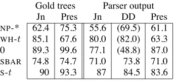
5.7 Comparison to Shen (2006) . . . 75
5.7.1 Difficulties in Comparing Results . . . 75
5.7.2 Results . . . 77
6 System Analysis 79 6.1 Error Analysis . . . 79
6.1.1 Nominal null wh-words . . . 79
6.1.2 Adverbial null wh-words . . . 80
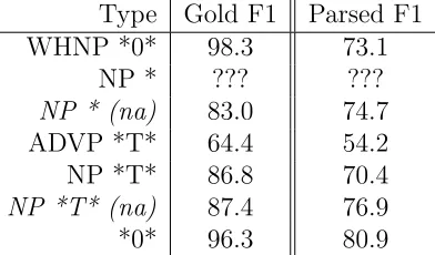
6.1.3 Nominal wh-traces . . . 82
6.1.4 Adverbial Trace (ADVP *T*) . . . 87
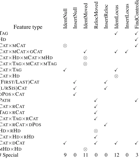
6.2 Feature Ablation . . . 89
7 Parsing With Google 99 7.1 The Google Web 1T Corpus . . . 99
7.2 Nullwh-word types . . . 100
7.2.1 Approach . . . 101
7.2.2 Results . . . 103
7.3 Infinitival Relatives . . . 104
7.3.1 Applying Google to the Problem . . . 109
7.3.2 Results . . . 114
7.4 Conclusions . . . 115
8 Conclusions and Future Work 117 8.1 Contributions . . . 117
8.2 Future Work . . . 118
A Evaluation 119 A.1 Johnson’s metric . . . 119
A.2 Campbell’s metric . . . 120
A.3 Typed–dependency metrics . . . 122
A.4 Typed Dependency Metric Implementation . . . 125
List of Tables
1.1 Frequencies of the most common null elements in English . . . 4
2.1 The performance of Johnson’s system, by his metric . . . 15
2.2 Dienes and Dubey’s null element performance. . . 21
2.3 Null element performance of Levy and Manning’s system . . . 28
2.4 Null element performance of Levy and Manning’s system (typed-dependency) . . . 28
3.1 List of function tags in the Penn Treebank and their distribution. . . 37
3.2 System performance on gold standard trees. . . 38
3.3 System performance on parser output. . . 39
3.4 System performance compared to Dienes and Dubey . . . 40
3.5 System performance compared to Campbell’s rules. . . 40
3.6 A few of the most important features for various classifiers. . . 41
4.1 The relative distribution of the most common null elements in Arabic and English. . . 44
4.2 The distribution of nominalwh-traces by type of relative clause in the Arabic Treebank training section . . . 46
4.3 Function tagging confusion matrix for Arabic. . . 57
4.4 Overall dependency evaluation for Arabic. . . 58
4.6 Performance for null element placement in Arabic for the system of Bakr et al. (2009) . . . 59
5.1 Gold standard and automatically-parsed test set results (F-measure) for the new and old English models by the typed-dependency metric. 74 5.2 Performance on wh-traces with overt wh-words compared to Shen
(2006). . . 77 5.3 Performance on wh-traces with empty wh-words compared to Shen
(2006) . . . 78
6.1 Descriptions of the feature classes . . . 97 6.2 This table shows how, beginning from a minimal base system, the
performance (F-measure) increases as feature classes are added in an order (roughly) from least complex to most complex. . . 98 6.3 This table shows how performance (F-measure) changes if each class
of feature is removed from the full system. . . 98
7.1 Distribution of wh-word type, overt and covert. . . 101 7.2 The counts used in determining the type of the nullwh-word in “the
man 0 I saw” . . . 102 7.3 The counts used in determining the type of the nullwh-word in “the
time 0 I went” . . . 102 7.4 Accuracy of the Google method onwh-type prediction. . . 104 7.5 Results on section 23 for the baseline, thresholding, parser, and
com-bined system approaches. . . 115 7.6 Change in the performance of null element placement when the
origi-nal pipeline (parser+system) is augmented with Web 1T informa-tion (combined+system) . . . 115
List of Figures
1.1 An example parse tree. . . 2
1.2 An example parse tree with null elements. . . 2
1.3 An example of a raising construction. . . 5
1.4 An example of a subject control construction. . . 5
1.5 An example of an object control construction. . . 6
1.6 Examples of nominal and adverbialwh-traces. . . 7
1.7 Examples of nullwh-words . . . 7
1.8 Examples of topicalization of NP and VP. . . 8
1.9 Examples of “permanent predictable ambiguity.” . . . 9
1.10 Examples of right node raising. . . 10
1.11 Examples of “insert constituent here.” . . . 10
1.12 Examples of expletive it. . . 10
2.1 One of Johnson’s patterns . . . 13
2.2 A diagram illustrating the idea of gap propagation as used in Model 3 of Collins (1999). . . 17
2.3 An example of gap-threading . . . 19
2.4 Campbell’s pipeline of rules . . . 23
2.5 Campbell’s rule for inserting (NP *) . . . 23
2.6 Features used by Levy and Manning . . . 27
4.2 Key for explanatory figures for graph creation. Boxes represent
vari-ables and circles represent factors. . . 51
4.3 Arabic graph example, part 1 . . . 51
4.4 Arabic graph example, part 2 . . . 52
4.5 An example of a trace with a resumptive pronoun within a -PRD. . . . 52
5.1 Gold standard analysis for an example where the original model erro-neously assigns NP *T* where NP *should be. . . 62
5.2 The erroneous original system analysis with an NP *T* where NP * should be. . . 62
5.3 A trace in the subject position of an infinitival relative. . . 63
5.4 Key for explanatory figures for graph creation (English) . . . 66
5.5 Adding slot and wh-type variables (English) . . . 67
5.6 Adding slot and wh-type variables (English) . . . 68
5.7 Adding wh-path factors . . . 69
5.8 A case of an (NP *) where the head word of the nearby ADJP-PRD indicates there is no coindexation. . . 74
5.9 A sample output tree from binc (from the dev-test section) . . . 76
6.1 An example of an error classed as “significant parser failure.” . . . 80
6.2 Chart showing distribution of errors for nominal null wh-words . . . . 81
6.3 An example where the parser analysis (above) appears superior to the analysis of the gold standard (below). The gold-standard analysis would imply that the calls were instrumental in stripping the stock markets. . . 82
6.4 Chart showing distribution of errors for adverbial nullwh-words . . . 83
6.5 A case of the parser erroneously inserting a relative clause due to the presence of time. Note that the tendency to place a relative clause after time is so strong it even outweighs the cost of using a rareVP → NN VP rule. . . 83 6.6 A case in which the trace placement is correct, but the metric counts
it wrong because the parser was mistaken about the parent symbol. The parser/system output is above and the gold standard is below. . 84
6.7 A case where the parser erroneously analyzes that as IN rather than WHNP. . . 85
6.8 A case where the parser fails to properly analyze a complex WHNP. . 85
6.9 A case where a simpleWHNPis incorrectly analyzed as if it were a more complexWHPP. . . 85
6.10 One of the few “miscellaneous” errors. . . 86
6.11 Here the parser erroneously creates a relative clause where none should be. The system output is above and the gold standard analysis is below. 86
6.12 Here call should have been parsed as having an S complement. The parser/system analysis is above and the gold standard is below. . . . 87
6.13 Here the parser pulls should and one down into a VP. The system has such a strong inclination against allowing subjectless VPs that it incorrectly places the trace. The parser/system analysis is above and the gold standard is below. . . 88
6.14 Here the parser marks these days as an argument when it should be an adjunct with a -TMP function tag. Therefore the system sees do’s subcategorization frame as filled and falls back to placing the trace in subject position. . . 88
6.15 This is the only remaining case of (NP *T*)/(NP *) confusion in the development test section. . . 89
6.17 A case where the gold standard analysis (shown) is wrong and the
system output (not shown) is correct. . . 91
6.18 A case where the system output, though differing from the gold stan-dard, is plausible. . . 92
6.19 In this case the trace dependencies in the system output (below; gold is above) are correct, but since the parser puts clean and repair in separateVPs, our second trace is counted as incorrect. . . 93
6.20 A case where the gold standard analysis (shown) does not coindex a wh-word, but our system does. . . 94
6.21 A more complicated case where the system output (below) has a trace for awh-word which lacks one in the gold-standard (above). Note that the system currently does not handle right-node raising. . . 95
6.22 Chart showing distribution of errors for adverbial wh-traces . . . 96
7.1 An example relative clause. . . 100
7.2 An example relative clause with a null wh-word. . . 100
7.3 The accuracy of determining nullwh-word types on the training data as a function of the thresholdα . . . 103
7.4 An infinitival relative. . . 105
7.5 An infinitive acting as anS modifier of a verb. . . 105
7.6 An infinitive acting as the complement of a noun. . . 106
7.7 Plot of all cases of infinitival Ss attaching to verbs. . . 111
7.8 Plot of all cases of infinitival Ss attaching as noun complements. . . . 112
7.9 Plot of all cases of infinitival Ss attaching to nouns as relative clauses. 113 A.1 Example of an ambiguity in Johnson’s metric, part 1 . . . 121
A.2 Example of an ambiguity in Johnson’s metric, part 2 . . . 121
A.3 An example where Campbell’s metric would count a null element as incorrect due to an attachment error in the antecedent. . . 123
Chapter 1
Introduction
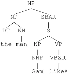
The field of natural language processing has achieved a high degree of accuracy in parsing (assigning syntactic structures to sentences, as in Figure 1.1), at least in English. Understanding the syntactic structure of a sentence is a necessary prelim-inary to understanding its semantics and therefore for many practical applications. However, the syntactic structures produced by the most commonly used parsers1 are less detailed than those structures found in the treebanks the parsers were trained on.
In particular, the parsers do not recover two sorts of information present in all the Penn Treebanks (English, Arabic, Chinese, and historical). The first are annotations on constituents indicating their syntactic or semantic function in the sentence (Gabbard et al., 2006). For example, the parser will label a noun phrase in its output as simply NP, but the treebank annotation would distinguish an NP-SBJ acting as the subject of a sentence from an NP-TMP (e.g. “tomorrow,” “next week”) acting as a temporal adjunct.
The second kind of information, which the proposed dissertation will focus on, are tree nodes which do not correspond to overt (written or pronounced) words. Such
1In particular, this is true of Collins (1999), Bikel (2004), and Charniak (2000), which are very
commonly used. Parsers designed for richer formalisms like LFG, TAG, and CCG do generally provide more detailed output, but they lie outside the scope of this work.
NP NP DT the NN man SBAR WHNP-1 -NONE-0 S NP NNP Sam VP VBZ t likes NP -NONE-*T*-1
Figure 1: A tree containing empty nodes.
in Figure 2 and modifies it by inserting empty nodes and coindexation to produce a the tree shown in Fig-ure 1. The algorithm is described in detail in sec-tion 2. The standard Parseval precision and recall measures for evaluating parse accuracy do not mea-sure the accuracy of empty node and antecedent re-covery, but there is a fairly straightforward extension of them that can evaluate empty node and antecedent recovery, as described in section 3. The rest of this section provides a brief introduction to empty nodes, especially as they are used in the Penn Treebank.
Non-local dependencies and displacement phe-nomena, such as Passive and WH-movement, have been a central topic of generative linguistics since its inception half a century ago. However, current linguistic research focuses on explaining the pos-sible non-local dependencies, and has little to say about how likely different kinds of dependencies are. Many current linguistic theories of non-local dependencies are extremely complex, and would be difficult to apply with the kind of broad coverage de-scribed here. Psycholinguists have also investigated certain kinds of non-local dependencies, and their theories of parsing preferences might serve as the basis for specialized algorithms for recovering cer-tain kinds of non-local dependencies, such as WH dependencies. All of these approaches require con-siderably more specialized linguitic knowledge than the pattern-matching algorithm described here. This algorithm is both simple and general, and can serve as a benchmark against which more complex ap-proaches can be evaluated.
NP NP DT the NN man SBAR S NP NNP Sam VP VBZ t likes
Figure 2: A typical parse tree produced by broad-coverage statistical parser lacking empty nodes.
The pattern-matching approach is not tied to any particular linguistic theory, but it does require a tree-bank training corpus from which the algorithm ex-tracts its patterns. We used sections 2–21 of the Penn Treebank as the training corpus; section 24 was used as the development corpus for experimen-tation and tuning, while the test corpus (section 23) was used exactly once (to obtain the results in sec-tion 3). Chapter 4 of the Penn Treebank tagging guidelines (Bies et al., 1995) contains an extensive description of the kinds of empty nodes and the use of co-indexation in the Penn Treebank. Table 1 contains summary statistics on the distribution of empty nodes in the Penn Treebank. The entry with POS SBAR and no label refers to a “compound” type of empty structure labelledSBARconsisting of an empty complementizer and an empty (moved)S (thusSBARis really a nonterminal label rather than a part of speech); a typical example is shown in Figure 3. As might be expected the distribution is highly skewed, with most of the empty node tokens belonging to just a few types. Because of this, a sys-tem can provide good average performance on all empty nodes if it performs well on the most frequent types of empty nodes, and conversely, a system will perform poorly on average if it does not perform at least moderately well on the most common types of empty nodes, irrespective of how well it performs on more esoteric constructions.
2 A pattern-matching algorithm
This section describes the pattern-matching algo-rithm in detail. In broad outline the algoalgo-rithm can
Figure 1.1: A parse of the noun phrase “the man Sam likes,” without null elements (Figure from Johnson)
NP NP DT the NN man SBAR WHNP-1 -NONE-0 S NP NNP Sam VP VBZ t likes NP -NONE-*T*-1
Figure 1: A tree containing empty nodes.
in Figure 2 and modifies it by inserting empty nodes and coindexation to produce a the tree shown in Fig-ure 1. The algorithm is described in detail in sec-tion 2. The standard Parseval precision and recall measures for evaluating parse accuracy do not mea-sure the accuracy of empty node and antecedent re-covery, but there is a fairly straightforward extension of them that can evaluate empty node and antecedent recovery, as described in section 3. The rest of this section provides a brief introduction to empty nodes, especially as they are used in the Penn Treebank.
Non-local dependencies and displacement phe-nomena, such as Passive and WH-movement, have been a central topic of generative linguistics since its inception half a century ago. However, current linguistic research focuses on explaining the pos-sible non-local dependencies, and has little to say about how likely different kinds of dependencies are. Many current linguistic theories of non-local dependencies are extremely complex, and would be difficult to apply with the kind of broad coverage de-scribed here. Psycholinguists have also investigated certain kinds of non-local dependencies, and their theories of parsing preferences might serve as the basis for specialized algorithms for recovering cer-tain kinds of non-local dependencies, such as WH dependencies. All of these approaches require con-siderably more specialized linguitic knowledge than the pattern-matching algorithm described here. This algorithm is both simple and general, and can serve as a benchmark against which more complex
ap-NP NP DT the NN man SBAR S NP NNP Sam VP VBZ t likes
Figure 2: A typical parse tree produced by broad-coverage statistical parser lacking empty nodes.
The pattern-matching approach is not tied to any particular linguistic theory, but it does require a tree-bank training corpus from which the algorithm ex-tracts its patterns. We used sections 2–21 of the Penn Treebank as the training corpus; section 24 was used as the development corpus for experimen-tation and tuning, while the test corpus (section 23) was used exactly once (to obtain the results in sec-tion 3). Chapter 4 of the Penn Treebank tagging guidelines (Bies et al., 1995) contains an extensive description of the kinds of empty nodes and the use of co-indexation in the Penn Treebank. Table 1 contains summary statistics on the distribution of empty nodes in the Penn Treebank. The entry with POS SBAR and no label refers to a “compound” type of empty structure labelledSBARconsisting of an empty complementizer and an empty (moved)S (thusSBARis really a nonterminal label rather than a part of speech); a typical example is shown in Figure 3. As might be expected the distribution is highly skewed, with most of the empty node tokens belonging to just a few types. Because of this, a sys-tem can provide good average performance on all empty nodes if it performs well on the most frequent types of empty nodes, and conversely, a system will perform poorly on average if it does not perform at least moderately well on the most common types of empty nodes, irrespective of how well it performs on more esoteric constructions.
2 A pattern-matching algorithm
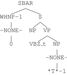
This section describes the pattern-matching algo-Figure 1.2: A parse of the same noun phrase which includes null elements (algo-Figure
from Johnson)
nodes are often (though not always) associated with other (overt or covert) nodes in the tree by means of bearing common numerical indices (see figure 1.2).2 These nodes serve several purposes (discussed in detail below), but the most important is to indicate non-local relationships between words and phrases which cannot be encoded the context-free constituent structure produced by the parser: the null element indicates that the co-indexed constituent, which may be far away, should be interpreted as if it were in the element’s position. As Levy and Manning (2004) point out, since these non-local relationships are important for semantics, it is necessary that either a way be found to enrich CFG parser output with this information or else it will be necessary to move to parsers explicitly designed for deeper syntactic frameworks (as they put it, the question is whether “the context-free parsing model is a safe approximation”). This information is also of more immediate practical value, with potential benefit for anything using predicate–argument structures of some sort, including question answering and textual entailment.
In the remainder of this chapter, we will discuss the types of null elements found in English. In the following two chapters we will address the tricky question of how to evaluate this task and what approaches other researchers have tried. In the next chapter, drawing on the insights of previous work, we will present a system for the task in English. In the next chapter we will examine the problem in Arabic, which motivates the creation of a new model for the problem which, in the next chapter, we apply to English. We conclude with a chapter examining some ways of using a large corpus of unlabeled data to mitigate parser errors which cause problems for null element restoration.
Null element Frequency
(NP *) → NP 18,334
(NP *) 9,812
(NP *T*) → WHNP 8,620
*U* 7,478
0 5,635
(S *T*)→ S 4,063
(ADVP *T*) → WHADVP 2,492
(SBAR *T*)→ S 2,033
(WHNP 0) 1,759
(WHADVP 0) 575
Table 1.1: The frequencies of the most common null elements in sections 2-21 of the Penn Treebank (data from Johnson). Those of the formX →Y mean a null element of type X co-indexed with an antecedent of type Y.
1.1
Null Elements in the Penn Treebank
1.1.1
Units
The unit element *U* is used to indicate null units of measure, especially monetary ones (Bies et al., 1995, 4.5.1).3 Most often, they correspond to where a currency word is placed when a text is read aloud, e.g. “$1,000,000 *U*” is pronounced “one-million dollars.” There are a few more (relatively rare) complex cases for the placement and usage of units (see the guidelines). Although they are the third most common type of null element, some systems ignore them because they can be restored pretty well by simple rules and do not create non-local dependencies.
2In the Treebank II format, the index is borne by the terminal symbol of the null element and
the non-terminal symbol of what it is coindexed with. In later versions of the annotation guidelines, indices are always placed on non-terminal symbols.
3Unless it is stated otherwise, all references in this section are to the Treebank II Guidelines
4 NULL ELEMENTS 73
4.3.4 Subjects of infinitival clauses
With coindexation
1. VP complement clauses.
Note that from the perspective of the annotator, it is not necessary to distinguish between Raising and Control structures, etc. In each case, the annotator simply coindexes the empty subject of the infinitival with whatever lexical NP it is associated with.
(a) “Raising” constructions. (S (NP-SBJ-3 Everyone)
(VP seems
(S (NP-SBJ *-3) (VP to
(VP dislike
(NP Drew Barrymore))))))
(b) “Object control” constructions.
(S (NP-SBJ Ford) (VP persuaded
(NP-1 Zaphod) (S (NP-SBJ *-1)
(VP to (VP run
(PP-CLR for
(NP president)))))))
(c) “Subject control” constructions. (S (NP-SBJ-1 Zaphod)
(VP promised (NP Ford) (S (NP-SBJ *-1)
(VP to (VP run
(PP-CLR for
(NP president)))))))
(d) Semi-auxiliaries.
Semi-auxiliaries occur in constructions with infinitival to, (e.g, supposed to, ought to, have to). They are annotated with full infinitival structure and have a (NP-SBJ *) subject, coindexed as appropriate.
(S (PP Of (NP course)) ,
(NP-SBJ-1 regulators) (VP would
(VP have
(S (NP-SBJ *-1) (VP to
(VP approve
(NP (NP Columbia ’s)
Figure 1.3: An example of (NP *) in a raising construction. Here the(NP *) marks that the proposition which seems to be the case is “everyone dislikes Drew Bar-rymore.” (This and all following examples in figures in this section are from the annotation guidelines)
4 NULL ELEMENTS 73
4.3.4 Subjects of infinitival clauses
With coindexation
1. VP complement clauses.
Note that from the perspective of the annotator, it is not necessary to distinguish between Raising and Control structures, etc. In each case, the annotator simply coindexes the empty subject of the infinitival with whatever lexical NP it is associated with.
(a) “Raising” constructions. (S (NP-SBJ-3 Everyone)
(VP seems
(S (NP-SBJ *-3) (VP to
(VP dislike
(NP Drew Barrymore))))))
(b) “Object control” constructions. (S (NP-SBJ Ford)
(VP persuaded (NP-1 Zaphod) (S (NP-SBJ *-1)
(VP to (VP run
(PP-CLR for
(NP president)))))))
(c) “Subject control” constructions.
(S (NP-SBJ-1 Zaphod) (VP promised
(NP Ford) (S (NP-SBJ *-1)
(VP to (VP run
(PP-CLR for
(NP president)))))))
(d) Semi-auxiliaries.
Semi-auxiliaries occur in constructions with infinitivalto, (e.g, supposed to, ought to, have to). They are annotated with full infinitival structure and have a (NP-SBJ *) subject, coindexed as appropriate.
(S (PP Of (NP course)) ,
(NP-SBJ-1 regulators) (VP would
(VP have
(S (NP-SBJ *-1) (VP to
(VP approve
(NP (NP Columbia ’s)
Figure 1.4: An example of (NP *) in a subject control construction. Here the (NP *) captures that Zaphod is promising thatZaphod (not Ford) will run for president.
1.1.2
Null Complementizers
In English, complementizers (roughly, words that introduce subordinate clauses) can often be omitted; these omitted complementizers are annotated as 0 (4.4). For example, you can say “I hope that dinner is ready” or “I hope 0 dinner is ready.” Like units, null complementizers are not especially interesting because they do not mediate non-local dependencies. However, there is an interesting and important subset of null complementizers, the null wh-words, which will be discussed below (1.1.4) with wh-movement.
1.1.3
PROs
The most frequent null element in the English treebank, (NP *) (which we will call PRO), has many uses. The simplest (arbitrary PRO) is as the subject of imperatives
4 NULL ELEMENTS 73
4.3.4 Subjects of infinitival clauses
With coindexation
1. VP complement clauses.
Note that from the perspective of the annotator, it is not necessary to distinguish between Raising and Control structures, etc. In each case, the annotator simply coindexes the empty subject of the infinitival with whatever lexical NP it is associated with.
(a) “Raising” constructions. (S (NP-SBJ-3 Everyone)
(VP seems
(S (NP-SBJ *-3) (VP to
(VP dislike
(NP Drew Barrymore))))))
(b) “Object control” constructions. (S (NP-SBJ Ford)
(VP persuaded (NP-1 Zaphod) (S (NP-SBJ *-1)
(VP to (VP run
(PP-CLR for
(NP president)))))))
(c) “Subject control” constructions. (S (NP-SBJ-1 Zaphod)
(VP promised (NP Ford) (S (NP-SBJ *-1)
(VP to (VP run
(PP-CLR for
(NP president)))))))
(d) Semi-auxiliaries.
Semi-auxiliaries occur in constructions with infinitivalto, (e.g, supposed to, ought to, have to). They are annotated with full infinitival structure and have a (NP-SBJ *) subject, coindexed as appropriate.
(S (PP Of (NP course)) ,
(NP-SBJ-1 regulators) (VP would
(VP have
(S (NP-SBJ *-1) (VP to
(VP approve
(NP (NP Columbia ’s)
Figure 1.5: An example of (NP *) in an object control construction. Here the (NP *) captures that Ford persuaded Zaphod that Zaphod (not Ford) should run for president.
(“(NP *) Go away!”)4 and in constructions where there is an understood pronoun of arbitrary reference, like “It is tough(NP *) to think carefully about St. Anselm’s ontological argument.” The second and most common use is to mark passivization, as in “(NP-1 Dante) was led (NP *-1) by Virgil.” The third primary use of PRO is in what linguists call control and raising constructions, for which see figures 1.3, 1.4, and 1.5. For the less common uses of PRO, see section 4.3 in the guidelines.
1.1.4
Wh
-movement
Traces ofwh-movement ((NP *T*)with antecedents of categoryWHNP,WHADVP,WHADJP, and WHPP) are used in the closely-related instances of questions and relative clauses to indicate in which argument or adjunct position thewh-word should be interpreted (4.2). For examples, see figure 1.6.
Closely related to them are those instances of null complementizers that replace wh-words in relative clauses (see figure 1.7).5 Determining that there is a missing
wh-word is not hard, but determining if it is nominal or adverbial is a challenging problem for null element restoration systems.
4School grammar sometimes calls this the “understood you.”
5These nullwh-words also occur in some places overtwh-words cannot, such as infinitival
4 NULL ELEMENTS 63
(ADVP-PRP *T*-54))) ?)
4.2.2 Relative clauses
Relative clauses are adjoined to the head noun phrase. The relative pronoun is given the appropriate WH-label, put inside the SBAR level, and coindexed with a *T* in the position of the gap. (Note that relative clauses differ from (direct)wh-questions in that they contain an SBAR rather than an SBARQ.)
wh- and “that” relative clauses. Relative clauses introduced by that are annotated just as relative clauses introduced by a wh-word: that is given the appropriate WH-label, put inside an SBAR level, and coindexed with the *T* in the position of the gap.
• NP trace
(NP (NP answers)
(SBAR (WHNP-6 that/which) (S (NP-SBJ-3 we)
(VP ’d (VP like
(S (NP-SBJ *-3) (VP to
(VP have
(NP *T*-6)))))))))
• ADVP trace
(NP (NP the place)
(SBAR (WHADVP-2 that/where) (S (NP-SBJ I)
(VP put
(NP the book)
(ADVP-PUT *T*-2)))))
Zero relatives. Relative clauses introduced by a null complementizer are annotated in a similar fashion, this time with a null complementizer ‘0’ inside SBAR labeled with the appropriatewh-category and coindexed with a *T* in the position of the gap.
• NP trace
(NP (NP answers) (SBAR (WHNP-3 0)
(S (NP-SBJ-4 we) (VP ’d
(VP like
(S (NP-SBJ *-4) (VP to
(VP have
(NP *T*-3)))))))))
Figure 1.6: Examples of nominal and adverbial wh-traces.
4 NULL ELEMENTS 64
• ADVP trace
(NP (NP the place) (SBAR (WHADVP-2 0)
(S (NP-SBJ I) (VP put
(NP the book)
(ADVP-PUT *T*-2)))))
Infinitival relatives. See section 14 [Infinitives] for more information.
• trace as object
(NP (NP a movie) (SBAR (WHNP-1 0)
(S (NP-SBJ *) (VP to
(VP see
(NP *T*-1))))))
• trace as subject
(NP (NP bloodhounds) (SBAR (WHNP-4 0)
(S (NP-SBJ *T*-4) (VP to
(VP trail
(NP the assassins))))))
• trace as adjunct
(NP (NP time)
(SBAR (WHADVP-1 0) (S (NP-SBJ *)
(VP to (VP go
(ADVP-TMP *T*-1))))))
4.2.3 Fronted elements
Fronted elements are placed inside the top clause level (e.g. S, SINV, SQ, SBAR). (Only certain fronted elements are tagged -TPC: (i) constituents associated with a *T* in the position of the gap and (ii) left-dislocated constituents (those associated with a resumptive pronoun in the position of the gap).) (See section 1 [Overview of Basic Clause Structure] for more details on the treatment of fronted elements.)
4 NULL ELEMENTS 64
• ADVP trace
(NP (NP the place) (SBAR (WHADVP-2 0)
(S (NP-SBJ I) (VP put
(NP the book)
(ADVP-PUT *T*-2)))))
Infinitival relatives. See section 14 [Infinitives] for more information.
• trace as object (NP (NP a movie)
(SBAR (WHNP-1 0) (S (NP-SBJ *)
(VP to (VP see
(NP *T*-1))))))
• trace as subject
(NP (NP bloodhounds) (SBAR (WHNP-4 0)
(S (NP-SBJ *T*-4) (VP to
(VP trail
(NP the assassins))))))
• trace as adjunct (NP (NP time)
(SBAR (WHADVP-1 0) (S (NP-SBJ *)
(VP to (VP go
(ADVP-TMP *T*-1))))))
4.2.3 Fronted elements
Fronted elements are placed inside the top clause level (e.g. S, SINV, SQ, SBAR). (Only certain fronted elements are tagged -TPC: (i) constituents associated with a *T* in the position of the gap and (ii) left-dislocated constituents (those associated with a resumptive pronoun in the position of the gap).) (See section 1 [Overview of Basic Clause Structure] for more details on the treatment of fronted elements.)
Figure 1.7: Examples of null wh-words. On the top is an ordinary relative clause and on the bottom is a infinitival relative.
4 NULL ELEMENTS 65
Arguments.
Fronted argument noun phrases are coindexed with a *T* in the position of the gap: (S (NP-TPC-3 This)
(NP-SBJ every man) (VP contains
(NP *T*-3)
(PP-LOC-CLR within (NP him))))
(S (NP-TPC-4 Our dull unsystematic youth) (NP-SBJ we)
(VP let
(S (NP-SBJ *T*-4) (VP stray
(PP-DIR into
(NP philanthropy))))))
If the fronted argument is an instance of left-dislocation (i.e, associated with a resumptive pronoun), there is no coindexation between the fronted argument and the pronoun:
(S (NP-TPC John) ,
(NP-SBJ I) (VP like
(NP him)
(NP-ADV a lot)))
Other fronted arguments (such as the main VP, a predicate, the locative complement ofput, etc.) are also tagged -TPC, and their identity index matches the reference index on the *T* inserted in the position of the gap.
(S (ADVP-PUT-TPC-1 There) ,
(NP-SBJ I) (VP put
(NP the book) (ADVP-PUT *T*-1)))
(S (SBAR-ADV (VP-TPC-2 Shout (PP-CLR at
(NP Eichmann))) though
(S (NP-SBJ he) (VP might
(VP *T*-2))))
the prosecutor could not establish...)
(S (SBAR-ADV (ADJP-PRD-TPC-5 Wrong) though
(S (NP-SBJ the policy) (VP may
4 NULL ELEMENTS 65
Arguments.
Fronted argument noun phrases are coindexed with a *T* in the position of the gap:
(S (NP-TPC-3 This) (NP-SBJ every man) (VP contains
(NP *T*-3)
(PP-LOC-CLR within (NP him))))
(S (NP-TPC-4 Our dull unsystematic youth) (NP-SBJ we)
(VP let
(S (NP-SBJ *T*-4) (VP stray
(PP-DIR into
(NP philanthropy))))))
If the fronted argument is an instance of left-dislocation (i.e, associated with a resumptive pronoun), there is no coindexation between the fronted argument and the pronoun:
(S (NP-TPC John) ,
(NP-SBJ I) (VP like
(NP him)
(NP-ADV a lot)))
Other fronted arguments (such as the main VP, a predicate, the locative complement ofput, etc.) are also
tagged -TPC, and their identity index matches the reference index on the *T* inserted in the position of the gap.
(S (ADVP-PUT-TPC-1 There) ,
(NP-SBJ I) (VP put
(NP the book) (ADVP-PUT *T*-1)))
(S (SBAR-ADV (VP-TPC-2 Shout (PP-CLR at
(NP Eichmann))) though
(S (NP-SBJ he) (VP might
(VP *T*-2))))
the prosecutor could not establish...)
(S (SBAR-ADV (ADJP-PRD-TPC-5 Wrong) though
(S (NP-SBJ the policy) (VP may
Figure 1.8: Examples of topicalization of NP and VP.
1.1.5
Topicalization
A *T* with other sorts of antecedents (e.g. NP, ADVP, VP, etc.) is used to indicate topicalization (4.2.3). Roughly, this is when an element is displaced from its usual position and put at the front of a sentence (see figure 1.8 for examples).
A particularly important subset of topicalization traces are the sentential traces, (S *T*), used to indicate when an S or SBAR from another part of a sentence oc-cupies an argument slot. They are used frequently for either direct ((S-1 ”I saw it yesterday”) she said (S *T*-1)) or indirect speech ((S-1 The files were lost), he claimed (SBAR 0 (S *T*-1))). Note that in the case of indirect speech, the structure is complicated by the trace being wrapped in an SBARtogether with a null complementizer (this is easy to understand if you “detransform” the sentence to “He claimed (SBAR that (S the files were lost)).”). Following Johnson, the whole SBAR in the indirect speech case is often treated as one big null element.
5 PSEUDO-ATTACH 101
5
Pseudo-Attach
5.1 Types of pseudo-attach
The pseudo-attach function is used for (1) structural ambiguity, (2) attachment in more than one place simultaneously, as with shared constituents, (3) indicating that something should be attached elsewhere, as with discontinuous dependencies, and (4) extraposed clauses. Each type of pseudo-attach is associated with a different type of null element (these are discussed in more detail in following sections; see also section 4 [Null Elements] for more information on indexing conventions):
1. Structural ambiguity *PPA* (“Permanent Predictable Ambiguity”) Example: I saw the man with the telescope, where *PPA*-attach indicates an either/or interpretation at the attachment sites.
(S (NP-SBJ I) (VP saw
(NP (NP the man) (PP *PPA*-1)) (PP-MNR-1 with
(NP the telescope))))
2. Shared constituents *RNR* (“Right Node Raising”)
Example: His dreams had revolved around her so much and for so long that..., where *RNR*-attach indicates a simultaneous interpretation at the attachment sites.
(S (NP-SBJ His dreams) (VP had
(VP revolved (PP-CLR around
(NP her))
(UCP-ADV (ADVP (ADVP so much) (SBAR *RNR*-1)) and
(PP-TMP for
(NP (NP so long) (SBAR *RNR*-1))) (SBAR-1 that...)))))
3. Discontinuous dependency *ICH* (“Interpret Constituent Here”) Example: I saw a bear yesterday who was wearing really cool shoes, where *ICH*-attach indicates that the relative clause is interpreted at the pseudo-attach site only.
(S (NP-SBJ I) (VP saw
(NP (NP a bear) (SBAR *ICH*-2)) (NP-TMP yesterday) (SBAR-2 (WHNP-1 who)
(S (NP-SBJ *T*-1) (VP was
Figure 1.9: Examples of a “permanent predictable ambiguity.” This is the classic example where “with the telescope” could, without a disambiguating context, modify “the man” or “saw.”
1.1.6
Ellipsed Predicates
*?* is used to indicate when it is not an argument or adjunct that has been moved or deleted, but rather a predicate (4.6) like a VP, PP-PRD, etc. This can happen in comparatives (“Acting would help him better than talking (VP *?*),” which is to say “Acting would help him better than talking would help him.”), conjunction (“Dianna likes tea, and I do (VP *?*)too”), and a variety of other cases (“Dianna likes tea, as do I (VP *?*)”). It is also used in some cases where the annotation guidelines do not otherwise specify how to fill the gap (the guidelines in section 4.6.3 give as an example “The plant cost about 50 million Canadian dollars to build (NP *?*)”).
1.1.7
Template gapping anti-placeholder
The last null element, *NOT*, is related to the interaction of gapping and coordi-nation. It will not be discussed here, since it is complicated, extremely rare, and probably impossible to recover automatically (4.7).
1.1.8
Pseudo-attachments
The annotation guidelines distinguish a certain class of null elements that represent shared or ambiguous attachments, calling them pseudo-attachments instead (5.1). There are four of these. First is*PPA*(permanent predictable ambiguity; figure 1.9)
5 PSEUDO-ATTACH 101
5
Pseudo-Attach
5.1 Types of pseudo-attach
The pseudo-attach function is used for (1) structural ambiguity, (2) attachment in more than one place simultaneously, as with shared constituents, (3) indicating that something should be attached elsewhere, as with discontinuous dependencies, and (4) extraposed clauses. Each type of pseudo-attach is associated with a different type of null element (these are discussed in more detail in following sections; see also section 4 [Null Elements] for more information on indexing conventions):
1. Structural ambiguity *PPA* (“Permanent Predictable Ambiguity”) Example: I saw the man with the telescope, where *PPA*-attach indicates an either/or interpretation at the attachment sites.
(S (NP-SBJ I) (VP saw
(NP (NP the man) (PP *PPA*-1)) (PP-MNR-1 with
(NP the telescope))))
2. Shared constituents *RNR* (“Right Node Raising”) Example: His dreams had revolved around her so much and for so long that..., where *RNR*-attach indicates a simultaneous interpretation at the attachment sites.
(S (NP-SBJ His dreams) (VP had
(VP revolved (PP-CLR around
(NP her))
(UCP-ADV (ADVP (ADVP so much) (SBAR *RNR*-1)) and
(PP-TMP for
(NP (NP so long) (SBAR *RNR*-1))) (SBAR-1 that...)))))
3. Discontinuous dependency *ICH* (“Interpret Constituent Here”) Example: I saw a bear yesterday who was wearing really cool shoes, where *ICH*-attach indicates that the relative clause is interpreted at the pseudo-attach site only.
(S (NP-SBJ I) (VP saw
(NP (NP a bear) (SBAR *ICH*-2)) (NP-TMP yesterday) (SBAR-2 (WHNP-1 who)
(S (NP-SBJ *T*-1) (VP was
Figure 1.10: Examples of right node raising. Here the trailing SBAR should be interpreted as modifying both “so much” and “so long.”
5 PSEUDO-ATTACH 107
(S (NP-SBJ *) (VP to
(VP (VP tear
(NP *RNR*-1)) and
(VP gnaw (PP-CLR on
(NP *RNR*-1))) (NP-1 his bones))))))
5.4 *ICH* (“Interpret Constituent Here”)
The most common type of pseudo-attach is *ICH*-attach, which is used to indicate a relationship of con-stituency between elements separated by intervening material. For instance, *ICH*-attach is used in “heavy shift” constructions when the movement results in a configuration in which it is impossible to attach the constituent to the phrase it belongs with:
(S (NP-SBJ (NP a young woman) (SBAR *ICH*-1)) (VP entered
(SBAR-1 (WHNP-2 whom) (S (NP-SBJ she)
(PP-TMP at
(ADVP once)) (VP recognized
(NP *T*-2) (PP-CLR as
(NP Jemima Broadwood)))))))
5.4.1 Word order
*ICH*-attach is never used solely to indicate word order; there must also be a difference in attachment height. For example, the following example does not require *ICH*-attach of the NP containinga very nice mermaid (here, because the sentence adverbial is attached in VP):
(S (NP-SBJ I) (VP met
(PP-LOC at
(NP the dock)) (NP (NP a
(ADJP very nice) mermaid)
(SBAR (WHNP-2 who)
(S (NP-SBJ-3 *T*-2) (VP offered
(S (NP-SBJ *-3) (VP to
(VP take (NP me) (PP-CLR for
(NP a swim)))))))))))
Figure 1.11: Examples of “insert constituent here.” Here, “a young woman whom she at once. . . ” has been split by the verb “entered.”
5 PSEUDO-ATTACH 102
(VP wearing
(NP (ADJP really cool) shoes)))))))
4. it-extraposition *EXP* (“EXPletive”)
Example:My teacher said it was OK for me to use the notes on the test, where *EXP*-attach indicates that the infinitive clause is the logical subject of the sentence.
(S (NP-SBJ My teacher) (VP said
(SBAR 0
(S (NP-SBJ (NP it)
(SBAR *EXP*-1)) (VP was
(ADJP-PRD OK) (SBAR-1 for
(S (NP-SBJ me) (VP to
(VP use
(NP the notes) (PP-LOC on
(NP the test)))))))))))
5.2 *PPA* (“Permanent Predictable Ambiguity”)
This form of pseudo-attach is reserved for those cases in which one cannot tell even from context where a constituent should be attached. Thedefaultis to attach the constituent at the more likely site (or if that is impossible to determine, at the higher site) and then to pseudo-attach it at all other plausible sites. Here,on the printercould modify eitherthe forms,the class or the forms, or it could go directly under VP as a PP adverbial. The PP in question is adjoined to the NPthe formsand *PPA*-attached to the other interpretation sites.
(S (NP-SBJ *) (VP Use
(NP this option)
(SBAR-TMP (WHADVP-2 when)
(S (NP-SBJ the operator) (VP changes
(NP (NP (NP the class) or
(NP (NP the forms) (PP-LOC-1 on
(NP the printer)))) (PP-LOC *PPA*-1))
(PP-LOC *PPA*-1) (ADVP-TMP *T*-2))))))
Figure 1.12: Examples of an expletive it. The null element indicates that this sen-tence is (basically) a rearranged version of “My teacher said for me to use the notes on the test was OK.”
which is used to indicate places where, even using the context, the annotator cannot distinguish the correct attachment of a constituent. It is used only where the different attachments actually change the meaning of the sentence (as opposed to “benign” ambiguities). It is rare and very unlikely to be automatically recoverable. Second, is *RNR* (right node raising; figure 1.10) which is used when a constituent needs to be interpreted in multiple places in the same sentence. Third and most common is
*ICH*(insert constituent here; figure 1.11), which is used when a constituent is split by other material being inserted into it. The last, *EXP* (expletive; figure 1.12) is used when a clause has been displaced with an “it” present where the clause should be interpreted.
1.2
Elements Under Consideration
Although we have above described many types of null elements in the Penn Treebank, many of them are quite rare. In this work, will will focus our attention (in English) on the nine non-unit categories in Table 1.1, since they account for the vast majority of the empty categories in the treebank.
Chapter 2
Related Work
There has been a considerable amount of previous work on the topic of null element restoration, beginning with Collins (1999) and Johnson (2002) and continuing in several directions. In this chapter, we will survey this previous work by grouping it by the four main approaches researchers have taken: patterns, parsing, rules, and machine learning. We will conclude by framing the approach taken in this thesis with respect to previous attempts.
2.1
Pattern-Matching
The seminal paper on the general null element problem is Johnson (2002). John-son’s approach, which he notes “may be regarded as an instance of . . . Memory-based Learning,” consists of extracting patterns from the Penn Treebank and then match-ing them against the trees we wish to restore null elements to. Johnson defines a pattern as a “minimal connected tree fragment containing an empty node and all nodes co-indexed with it.” A pattern P matches a tree T if T is an extension ofP
SBAR WHNP-1 -NONE-0 S NP VP
VBZ t NP
-NONE-*T*-1
Figure 4: A pattern extracted from the tree displayed in Figure 1.
accuracy of transitivity labelling was not systemati-cally evaluated here.
2.2 Patterns and matchings
Informally, patterns are minimal connected tree fragments containing an empty node and all nodes co-indexed with it. The intuition is that the path from the empty node to its antecedents specifies im-portant aspects of the context in which the empty node can appear.
There are many different possible ways of realiz-ing this intuition, but all of the ones tried gave ap-proximately similar results so we present the sim-plest one here. The results given below were gener-ated where the pattern for an empty node is the min-imal tree fragment (i.e., connected set of local trees) required to connect the empty node with all of the nodes coindexed with it. Any indices occuring on nodes in the pattern are systematically renumbered beginning with 1. If an empty node does not bear an index, its pattern is just the local tree containing it. Figure 4 displays the single pattern that would be extracted corresponding to the two empty nodes in the tree depicted in Figure 1.
For this kind of pattern we definepattern match-inginformally as follows. Ifpis a pattern and tis a tree, thenpmatchestifftis an extension ofp ig-noring empty nodes inp. For example, the pattern displayed in Figure 4 matches the subtree rooted un-derSBARdepicted in Figure 2.
If a pattern pmatches a treet, then it is possible tosubstitute pfor the fragment oftthat it matches. For example, the result of substituting the pattern
shown in Figure 4 for the subtree rooted underSBAR depicted in Figure 2 is the tree shown in Figure 1. Note that the substitution process must “standardize apart” or renumber indices appropriately in order to avoid accidentally labelling empty nodes inserted by two independent patterns with the same index.
Pattern matching and substitution can be defined more rigorously using tree automata (G´ecseg and Steinby, 1984), but for reasons of space these def-initions are not given here.
In fact, the actual implementation of pattern matching and substitution used here is considerably more complex than just described. It goes to some lengths to handle complex cases such as adjunction and where two or more empty nodes’ paths cross (in these cases the pattern extracted consists of the union of the local trees that constitute the patterns for each of the empty nodes). However, given the low frequency of these constructions, there is prob-ably only one case where this extra complexity is justified: viz., the empty compound SBAR subtree shown in Figure 3.
2.3 Empty node insertion
Suppose we have a rank-ordered list of patterns (the next subsection describes how to obtain such a list). The procedure that uses these to insert empty nodes into a tree t not containing empty nodes is as fol-lows. We perform a pre-order traversal of the sub-trees oft (i.e., visit parents before their children), and at each subtree we find the set of patterns that match the subtree. If this set is non-empty we sub-stitute the highest ranked pattern in the set into the subtree, inserting an empty node and (if required) co-indexing it with its antecedents.
Note that the use of a pre-order traversal effec-tively biases the procedure toward “deeper”, more embedded patterns. Since empty nodes are typi-cally located in the most embedded local trees of patterns (i.e., movement is usually “upward” in a tree), if two different patterns (corresponding to dif-ferent non-local dependencies) could potentially in-sert empty nodes into the same tree fragment int, the deeper pattern will match at a higher node int, and hence will be substituted. Since the substitu-tion of one pattern typically destroys the context for a match of another pattern, the shallower patterns no longer match. On the other hand, since shal-Figure 2.1: The pattern resulting from doing pattern extraction on shal-Figure 1.2 (shal-Figure
from Johnson)
2.1.1
The Training Phase
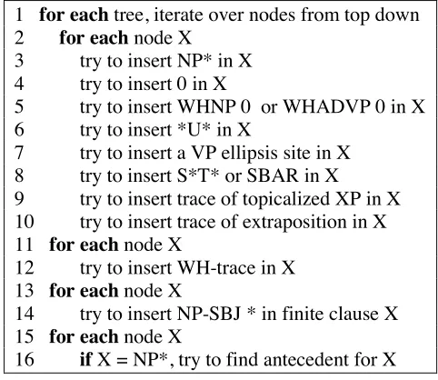
During the training phase, the system goes through each tree in the corpus and, for every null element, extracts the minimal connected tree which contains it and every node co-indexed with it (a pattern; see figure 2.1). If there are no nodes co-indexed with it, then its parent and siblings are extracted. At this point we have a list of patterns and how many times they each occurred (indicated by cp for a pattern p). This results in about 11,000 patterns.
Next, the system counts how many times each pattern matches in the treebank, called the match value (mp). Note that since matching ignores empty categories in the pattern, a pattern may match places in the treebank which are identical to it except for null elements. There are a number of ways to count the pattern matches for determining the match value. The simplest is just to count how many times each pattern matches when applied as often as possible without regard to other patterns. However, if one pattern is a subtree of another pattern (ignoring null elements), both will match, but it is not the case that both could actually be applied. Therefore the naive approach tends to favor “shallow” trees over “deep” trees. To fix this, the system walks through the nodes in a pre-order traversal, attempting to match
patterns at each. Afterward, it chooses whatever pattern would have been correct to apply, if any, and applies it, inserting the appropriate null elements (see section 2.1.2). The presence of these null elements may then block shallower patterns from being applied within the “domain” of this deeper pattern. Johnson notes that this change has a large effect on performance.
Having calculated the counts and match values, patterns are now pruned. This is necessary because some patterns would insert null elements incorrectly more often than they would correctly (that is, the success probability cp/mp < 12). For each pattern, a statistical technique is used to throw out those patterns we cannot be confident truly have a success probability greater than a half (this is needed because some rare patterns may have such a success probability observed in our training sample by accident). After pruning, about 9,000 patterns remain.
Finally, if more than one pattern can apply at a node, which should be chosen? The patterns are ranked by depth, and the system at runtime will prefer to apply deeper patterns before shallower ones. Johnson also notes that he tried ranking patterns by success probability with very similar results.
2.1.2
The Application Phase
To restore empty categories to a tree, the system does a pre-order traversal. At each node, it checks which patterns, if any, match and applies the highest ranked one. To apply a pattern, it replaces the matching subtree with the contents of the pattern, renumbering null element indices if necessary to prevent accidental collision with coindexation already in the tree.
2.1.3
The Preprocessor
Empty node Section 23 Parser output
POS Label P R f P R f
(Overall) 0.93 0.83 0.88 0.85 0.74 0.79 NP * 0.95 0.87 0.91 0.86 0.79 0.82 NP *T* 0.93 0.88 0.91 0.85 0.77 0.81 0 0.94 0.99 0.96 0.86 0.89 0.88 *U* 0.92 0.98 0.95 0.87 0.96 0.92 S *T* 0.98 0.83 0.90 0.97 0.81 0.88 ADVP *T* 0.91 0.52 0.66 0.84 0.42 0.56 SBAR 0.90 0.63 0.74 0.88 0.58 0.70 WHNP 0 0.75 0.79 0.77 0.48 0.46 0.47
Table 3: Evaluation of the empty node restoration procedure ignoring antecedents. Individual results are reported for all types of empty node that occured more than 100 times in the “gold standard” corpus (sec-tion 23 of the Penn Treebank); these are ordered by frequency of occurence in the gold standard. Sec(sec-tion 23 is a test corpus consisting of a version of section 23 from which all empty nodes and indices were removed. The parser output was produced by Charniak’s parser (Charniak, 2000).
Empty node Section 23 Parser output
Antecedant POS Label P R f P R f
(Overall) 0.80 0.70 0.75 0.73 0.63 0.68
NP NP * 0.86 0.50 0.63 0.81 0.48 0.60
WHNP NP *T* 0.93 0.88 0.90 0.85 0.77 0.80 NP * 0.45 0.77 0.57 0.40 0.67 0.50 0 0.94 0.99 0.96 0.86 0.89 0.88 *U* 0.92 0.98 0.95 0.87 0.96 0.92 S S *T* 0.98 0.83 0.90 0.96 0.79 0.87 WHADVP ADVP *T* 0.91 0.52 0.66 0.82 0.42 0.56 SBAR 0.90 0.63 0.74 0.88 0.58 0.70 WHNP 0 0.75 0.79 0.77 0.48 0.46 0.47
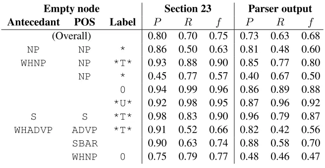
Table 4: Evaluation of the empty node restoration procedure including antecedent indexing, using the mea-sure explained in the text. Other details are the same as in Table 4.Table 2.1: The performance of Johnson’s system, by his metric (Table from Johnson)
More importantly, the part-of-speech tags of transitive verbs have a “ t” ap-pended to them. A verb is determined to be transitive if more than half the time it is followed by a noun phrase which does not carry a function tag marking it as a non-argument. Johnson notes than experiments on the development test set showed a small improvement from this annotation.
2.1.4
Evaluation
Results from the system can be see in table 2.1. The relative performance of the different null elements set the basic pattern for future work. Units, non-wh null complementizers, and sentential traces are recovered relatively well; nominal wh -traces moderately well; and adverbial -traces and null wh-words poorly. (NP *) proves easy to insert, but very difficult to find the antecedent for. Results from other systems, while having trouble in the same places, have generally been better. In part, this is likely due to Johnson’s patterns being less robust – both against parser errors and in the broader sense of generalizability – than later approaches.
2.1.5
“Looser” Pattern-Matching
Another system which uses some form of pattern-matching is Jijkoun and de Rijke (2004), which used memory-based learning. They will not be discussed in further detail here since they operate only on dependency structures and report scores very similar to Dienes and Dubey (2003b), who will be discussed next.1
2.1.6
Regular Expression Patterns
Filimonov and Harper (2007) present another pattern-based system which achieves significantly more robustness than Johnson’s by means of handwritten patterns (with automatically assigned probabilities) which are made more flexible in a manner rather analogous to regular expressions. Since this system is both rather compli-cated and very focused (limiting itself to onlywh-traces with overt antecedents), we will not discuss it in further detail here.
2.2
Parsing
It is appealing to attempt to recover null elements within the parser. After all, finding null elements is properly part of the task of syntactic analysis the parser is supposed to perform. Indeed, one of the seminal dissertations in modern parsing (Collins, 1999) treated the recovery of wh-traces in its third, most complex model. We will describe it briefly in this section under the assumption the reader is familiar with Collins’s Model 2; for those who are not, we refer them to Collins’s thesis.
Model 3 begins by annotating the training trees with gap annotations in the manner of Gazdar et al. (1985). For every non-terminal on the path between a
1It is not clear that their numbers are in fact comparable to those of Dienes and Dubey on
Figure 2.2: A diagram illustrating the idea of gap propagation as used in Model 3 of Collins (1999). Every node between the trace and its antecedent is annotated with +gap. Figure from Collins’s thesis.
trace and its antecedent, a +gap feature annotation is added. The parsing model is then modified to take this into account: in addition to indicating whether the usual constituents like NPs are expected, subcategorization frames can now also contain gaps. These gaps may be discharged either by producing a trace or by producing an ordinary non-terminal which has the+gapfeature, and the node and head generation probability models are modified accordingly. The question remains, however, of whether a symbol looking for a gap below it should add it to the left subcategorization frame, the right subcategorization frame, or neither (in which case the gap feature would be passed on to the immediate head of the symbol). This is modeled by the addition of a new probability distribution PG whose values are the three options above and which is conditioned on the parent symbol, head symbol, and head word.
In more recent work, Model 3 has been extended by Dienes and Dubey (2003b), which we will now consider. These authors propose two possible methods which we might call partial and full parser integration. In partial integration, a finite-state
method is applied to the surface string to insert null elements, and the sentence is then parsed treating the null elements just like they were normal words. In complete integration, there is no preliminary step, and null element insertion is done entirely in the parser.
2.2.1
Partial Integration
The first step in this approach is to use a finite-state “trace tagger” to mark the positions of the null elements in the surface string. Dienes and Dubey (2003a) had previously presented such a tagger which achieves a 79.1% F-score on null element detection. The tagger primarily employs three pieces of information:
• the part-of-speech tags in a five word window
• lexical features in a three word window
• non-local features which look through the string for signs of passives, to-infinitives, gerunds, wh-words, and “that.”
They note that the first class of features is their most informative.
The second step of this approach is to use a parser to find the antecedents of those null elements inserted in the first step. In order to do this they modify the training trees for the parser according to a variation of the gap-propagation technique described above: for every null element, every non-terminal node between it and (up to but not including) its antecedent’s parent has gap+<gap-type> appended to its label (for an example, see Figure 2.3). Note that a label may receive more than one gap annotation.