www.nat-hazards-earth-syst-sci.net/11/323/2011/ doi:10.5194/nhess-11-323-2011
© Author(s) 2011. CC Attribution 3.0 License.
Natural Hazards
and Earth
System Sciences
Nonlinear random wave field in shallow water:
variable Korteweg-de Vries framework
A. Sergeeva, E. Pelinovsky, and T. Talipova
Institute of Applied Physics, Nizhny Novgorod, Russia
Received: 27 September 2010 – Revised: 23 November 2010 – Accepted: 24 November 2010 – Published: 3 February 2011
Abstract. The transformation of a random wave field in shallow water of variable depth is analyzed within the framework of the variable-coefficient Korteweg-de Vries equation. The characteristic wave height varies with depth according to Green’s law, and this follows rigorously from the theoretical model. The skewness and kurtosis are computed, and it is shown that they increase when the depth decreases, and simultaneously the wave state deviates from the Gaussian. The probability of large-amplitude (rogue) waves increases within the transition zone. The characteristics of this process depend on the wave steepness, which is characterized in terms of the Ursell parameter. The results obtained show that the number of rogue waves may deviate significantly from the value expected for a flat bottom of a given depth. If the random wave field is represented as a soliton gas, the probabilities of soliton amplitudes increase to a high-amplitude range and the number of large-amplitude (rogue) solitons increases when the water shallows.
1 Introduction
Rogue or freak waves, which rapidly and surprisingly appear and disappear on the sea surface, are widely observed in various areas of the World Ocean in both open seas and coastal zones; such data is collected in Lavrenov (2003), Didenkulova et al. (2006), Liu (2007), Kharif et al. (2009). Several physical mechanisms are suggested to explain the rogue wave phenomenon (Dysthe et al., 2008; Kharif et al., 2009): (i) dispersive and geometrical focusing of wave packets propagating with different speeds in different directions; (ii) nonlinear mechanisms due to the Benjamin-Feir instability and wave-wave interaction; (iii) wave
Correspondence to: A. Sergeeva ([email protected])
interaction with a variable bottom, with currents and wind flow. These physical mechanisms are the subject of intense study in frameworks of various theoretical models of water waves and also through simulations in laboratory tanks; see for instance Kharif et al. (2009).
For practical purposes it is necessary to compute the probability of rogue wave occurrence. Usually, the distribution functions of the wind wave field including extreme characteristics are calculated under assumption of the non-Gaussian properties of a process using the nonlinear perturbation technique; see for instance Dysthe et al. (2008). The nonlinear effect of the Benjamin-Feir instability for narrow-band wave packets over deep water is incorporated in the statistical theory of the weak (wave) turbulence. It leads to the non-Gaussian statistics of wind waves with third and fourth moments (skewness and kurtosis) depending on the Benjamin-Feir index which represents the ratio of nonlinearity to dispersion (Janssen, 2003; Mori and Janssen, 2006). As a result, the probability of rogue wave occurrence increases due to the Benjamin-Feir instability and this effect has been verified experimentally in a long wave flume (Onorato et al., 2006; Shemer and Sergeeva, 2009; Shemer et al., 2010).
The influence of the combined effects of nonlinear – dispersive focusing of unidirectional random waves over shallow water (where the Benjamin-Feir instability is absent) on the probability of freak wave appearance has been studied within the Korteweg-de Vries equation (Pelinovsky and Sergeeva, 2006). In this case the wave field remains non-Gaussian, and the skewness and kurtosis are controlled by the Ursell parameter, which is proportional to the ratio of nonlinear over dispersive effects.
324 A. Sergeeva et al.: Nonlinear random wave field in shallow water wave propagation over variable bottom is concerned, the
wave characteristics are non-Gaussian; the runup of random long waves on a plane beach is one of these examples. The statistical moments for this case are studied theoretically in Didenkulova et al. (2008, 2011) and experimentally in Huntley et al. (1977).
The influence of the bathymetry non-uniformity on kurto-sis and the probability of freak waves has been investigated within the framework of the nonlinear Schr¨odinger equation in Zeng and Trulsen (2010). They found that after a depth variation, the propagating wave train may need a considerable distance to relax towards the new equilibrium state, which corresponds to the new depth. As a result, kurtosis and the number of freak waves may be significantly different from the values expected for the constant depth environment. This analysis is limited by the narrow-band dispersive wave packet under conditions at intermediate depth.
The main goal of the present paper is to investigate the effect of variable bathymetry on the unidirectional random wave propagation in shallow water. The theoretical model is based on the variable-coefficient Korteweg-de Vries equation (Sect. 2). If the wave field is represented by an ensemble of solitons with random amplitudes and phases, the distribution function of soliton heights is shown to grow in high-amplitude limit (the “tail” of the distribution function), and the number of “freak” solitons increases when the depth becomes less. The results of numerical simulations on propagation of initially random wave field under condition when water shallows, are given in Sect. 3. It is emphasized within this framework, that the freak wave probability should increase when depth decreases. The entrance of random waves to a deeper water region leads to the reduction of the number of freak waves, as discussed in Sect. 4. The results obtained are summarized in Sect. 5.
2 The Korteweg-de Vries model
The Korteweg-de Vries equation is a basic equation for describing a unidirectional propagation of weakly-nonlinear weakly-dispersive waves in shallow waters. In the case of a slowly variable depth when the wave reflection from the bottom slopes can be neglected, the variable-coefficient Korteweg-de Vries equation has been derived by Ostrovsky and Pelinovsky (1970), Johnson (1973). It can be written as p
gh(x)∂η ∂x+
3η 2h
h(x) h0
−1/4∂η ∂s+
h(x) 6g
∂3η
∂s3=0, (1) where the surface elevation ζ (x,t ) and the time t are introduced as follows,
ζ (x,t )=η(x,t ) h(x)
h0 −1/4
, s=
x
Z
x0 dy
√
gh(y)−t , (2)
sis the time in the reference system of coordinates,x is the coordinate directed onshore, h0=h(x0)is the depth of the deepest tide-gauge where an initial condition is defined.
Equation (1) is solved numerically for the periodic domain onswith the periodT,ζ (0,x)=ζ (T ,x). Two integrals of Eq. (1) are conserved,
T
Z
0
η(x,s)ds=const,
T
Z
0
η2(x,s)ds=const. (3)
The pseudo-spectral method for time derivation and the Crank-Nicolson scheme for space discretization are used, see details in Fornberg (1998). The solution of (1) is calculated in the discrete Fourier space for spectral amplitudes and defined through the Fourier transformC(ω)= FFT{η(s,x)}, when the nonlinear part of (1) is calculated asCnon(ω)= FFT
η2(s,x)/2
C (ω,x+1x)=C (ω,x−1x)1+iβω 31x
1−iβω31x
−αFFT 1
2η 2(s,x)
iω1x
1−iβω31x , (4a)
α= 3
2h√gh h
h0 −1/4
, β= h
6g√gh. (4b)
The initial conditions for (1) at x0=0 were defined as a superposition of independent Fourier harmonics with random phasesϕuniformly distributed within the interval [0 2π] ζ (s,x=0)=η(s,x=0)=X
n
p
2S (ωn)cos(ωns+ϕn) . (5)
The total duration of each realization is about 30 character-istic wave periods corresponding to the typical swell period T0=15 s and sample frequencyf =5.7 Hz (N= 1024 data points are used for the discretization in times). The spatial discretization in (4) is much less then a wave length and is equal to 1x=0.375h0. The spectrum of water waves at initial location was assumed to have a Gaussian shape S (ω)=A2exp
"
−
ω−ω 0 δω
2#
, (6)
The following variable depth profile is employed in the numerical experiments:
h(x)
h0 =
1+h1/ h0
2 −
1−h1/ h0
2 tanh(x/L) . (7)
Here the initial depthh0is set to 10 m, and the final depth wash1=5 m. The length of the transitional zone,L, varies from 30h0to 120h0(2–8 wavelengths).
The main goal of the numerical simulations is to find the wave field statistical moments. The first two statistical moments can be easily found analytically with the use of (3). In particular, the first moment is
m1(x)=
T
Z
0
ζ (x,s)ds
=
h(x) h0
−1/4ZT
0
η(x,s)ds∼
h(x) h0
−1/4
m1(x0) , (8)
Meanwhile, at the initial locationm1(x0)=0; therefore the mean water level does not change with distance. The second moment reads
m2(x)=σ2(x)=
T
Z
0
ζ2(x,s)ds
=
h(x)
h0
−1/2ZT
0
η2(x,s)ds∼
h(x)
h0 −1/2
m2(x0) . (9)
The characteristic wave amplitude (defined here as half of the significant wave height) is proportional to σ (x) as As(x)=2σ (x). It varies with depth according to Green’s lawh−1/4(x). The skewness and kurtosis defined as µ3(x)=m3(x)
σ3(x), µ4(x)= m4(x)
σ4(x) (10)
can not be obtained analytically, and are computed by means of numerical simulations.
Simple analytical results can be achieved for the case when the random field constitutes a “solitonic gas”. The soliton turbulence within the framework of the Korteweg-de Vries equation has specific features related to integrability: solitons preserve their individuality, and interactions between them are elastic, and thus do not change soliton amplitudes but alter phases, see Zakharov (1971), Salupere et al. (1996, 2002, 2003a, b), and textbooks Novikov et al. (1980), Drazin and Johnson (1996).
Assuming the random solitons to be located far from each other, the soliton transformation in the coastal zone (shoaling) may be analysed independently for every solitary wave. This dynamics is known to depend on the ratio of nonlinearity length with respect to the width of the
transition zone (Tappert and Zabusky, 1971; Pelinovsky, 1971; Nakoulima et al., 2005). If the solitary wave amplitude is large, the soliton quickly adapts to the local depth, so that its new length coincides with the local conditions. In this case the soliton amplitude is proportional to h−1(x); see Ostrovsky and Pelinovsky (1970), Johnson (1973). If the solitary wave has small amplitude, and thus, large wave length, it transforms as a linear wave, and its amplitude is proportional toh−1/4(x); see Pelinovsky (1971), Nakoulima et al. (2005). As a result, the distribution of soliton amplitudes changes with depth, and the portion of large-amplitude waves enhances more significantly than the portion of smaller-amplitude solitons.
Thus, the nonlinear property of the soliton field tends to increase the probability of occurrence of large-amplitude waves (freak waves). Of course, this analysis is limited by the low-density “soliton gas” representation of the wave field. In general, the wave field is represented by a superposition of sinusoidal waves with random phases (4), and the statistical moments are calculated numerically, as reported below.
3 Shoaling of random nonlinear waves
Let us suppose the region where the initial condition is defined to be far from the transitional zone. Then the Korteweg-de Vries equation for a constant depth may be employed. It is demonstrated in Pelinovsky and Sergeeva (2006) that during the nonlinear wave evolution, the Gaussianity of the process breaks down after a transitional period. Later on, a steady state is established (regarding statistical characteristics), which differs from the Gaussian state and is characterized by a stronger wave asymmetry and kurtosis, when the Ursell parameter grows. The Ursell parameter defines the ratio of nonlinearity As/h(x) with respect to dispersion [k0h(x)]2,
Ur(x)= As(x)
k02(x)h3(x)=
2σ (0)gh10/4
ω02h(x)9/4 , (11) where g is the gravity acceleration. Strictly speaking, the Ursell parameter is defined for a sinusoidal wave with frequencyω0.
Our simulations exhibit the spectrum broadening due to the nonlinearity effect; it also becomes asymmetrical, see Fig. 1 (see also, Pelinovsky and Sergeeva, 2006) and a second harmonic peak is observed. For estimating the Ursell parameter, we used the value ofω0, obtained on the basis of the initial Gaussian spectrum (6) through the spectral moments,
ω0= R
ωS (ω)dω R
S(ω)dω . (12)
326 A. Sergeeva et al.: Nonlinear random wave field in shallow water
Fig. 1. Power spectra of surface elevation atx=150h0 and at
x=300h0 for Ur = 0.4. Red solid line corresponds to the initial
Gaussian shaped spectrum. Constant depthh0=10 m.
(a)
(b)
(c)
8 a)
b)
c)
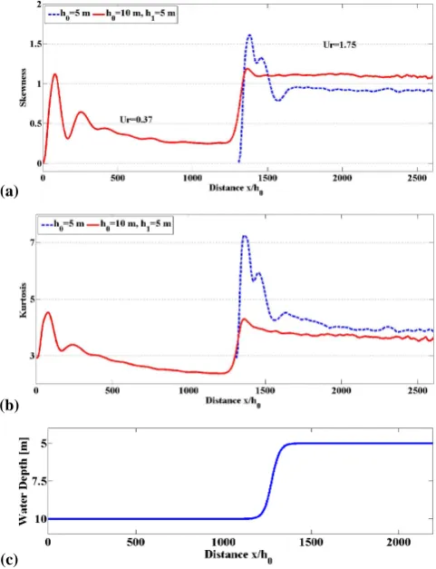
Figure 2. Variation of the skewness (a) and kurtosis (b) in the water of variable depth with initial value Ur = 0.37 (dashed line). The same variation in the water of constant depth h0 = 5 m with
Ur = 1.75 (solid line). Variable depth profile with L = 30h0 (c).
An increase of the wave steepness (ε= 1⋅10-2) leads, as expected, to more significant deviations
of the skewness and kurtosis from the values of the Gaussian state (Fig. 3). As opposed to the previous case (Ur = 1.75), the comparison with the simulation for a constant depth in the case of steeper waves (Ur = 3.5) manifests two different regimes of the steady state at the depth h = 5 m:
large transition zone for a constant depth condition and shorter transformation to a steady state Fig. 2. Variation of the skewness (a) and kurtosis (b) in the water
of variable depth with initial value Ur = 0.37 (solid line). The same variation in the water of constant depthh0=5 m with Ur = 1.75
(dashed line). Variable depth profile withL=30h0(c).
parameter equals to 0.37. Figure 2a and b indicates the spatial evolution of the statistical moments, the skewnessµ3 and kurtosis µ4, are marked with the red solid line. The variation of the water depth profile is presented in Fig. 2c.
While the depth is constant before the transitional zone, the quasi-stationary state for µ3 and µ4 is achieved (Pelinovsky and Sergeeva, 2006). It is characterized by the
(a)
(b)
(c)
9 for water with depth decrease. The results of calculations of the wave propagation over variable depth conditions demonstrate significant increase of the values of the kurtosis and skewness versus the case of a constant depth.
a)
b)
c)
Figure 3. As in Figure 1(a,b) for Ur = 0.7 and Ur = 3.5. Depth profile with L = 30h0 (c).
As it was already mentioned, the decrease of water depth leads to the growth of nonlinearity and Ursell parameter as well. It was shown (Figs 2,3) that statistical moments also tend to grow while the water shallows. All this influence the probability distribution of large wave formation and lead to the growth of the tails of distribution function after the transition zone. Figures 4(a,b) demonstrate such behaviour of probability distribution functions of wave height, scaled by Hs = Fig. 3. As in Fig. 1a and b for Ur = 0.73 and Ur = 3.47. Depth
profile withL=30h0(c).
increase of the wave asymmetry and by the growth of the number of high amplitudes in comparison with the Gaussian distribution; thus, the process deviates far from the Gaussian one. The water depth variation leads to the growth of the wave nonlinearity, and the Ursell parameter grows up to Ur = 1.75 as well. For the new condition, a new steady state can be observed at distances overx=1500h0.
For a comparison, the evolution of random waves with an initially Gaussian-shaped spectrum was considered for the condition of constant depth, h0=5 m, for the same value of the Ursell parameter, Ur = 1.75. These results were compared with the previous simulations in Fig. 2a and b (blue dashed lines correspond to the condition of constant depth). Both statistical moments tend to quite similar values in the two simulations.
A. Sergeeva et al.: Nonlinear random wave field in shallow water 327
(a)
10 4σ,, both for two case of initial values of wave steepness ε= 1⋅10-2 and ε= 5⋅10-3, where blue symbols correspond to the depth of 10 m and red symbols indicate the probabilities of wave heights in shallower water (h=5 m).
a)
b)
Figure 4. Exceedance probability distribution function of wave heights scaled by Hs for water depth h=10 m (blue symbols) and h=5 m (red symbols) for two cases of initial wave steepness:
ε=1⋅10-2 (a) and ε= 5⋅10-3(b).
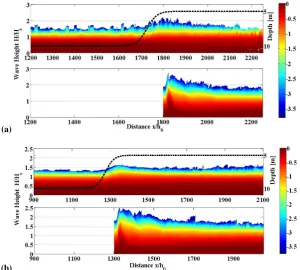
The spatial variation of the exceedance probability function for wave heights, log(F[H/Hs]), presented in spatial diagrams (H/Hs, x/h0) of Figs 5a,b, allows to indicate the formation of large waves along the distance for two cases examined above. The profile of the water depth is also given for the reference by the dashed line, and the right vertical axis indicates the depth values. For the comparison, the variations of the wave height probabilities obtained for the conditions of a constant water depth h = 5 m and the corresponding Ursell parameters are presented in Figs. 5a and 5b below the main panels.
For both sets of the numerical experiments the variation of water depth correlates with the evidence of formation of larger waves, which wave heights more then twice exceed the significant wave height, Hs, (so-called freak waves). A visible transient zone exists for the
(b)
10 = 1⋅10 = 5⋅10
symbols correspond to the depth of 10 m and red symbols indicate the probabilities of wave heights in shallower water (h=5 m).
a)
b)
Figure 4. Exceedance probability distribution function of wave heights scaled by Hs for water depth h=10 m (blue symbols) and h=5 m (red symbols) for two cases of initial wave steepness:
ε=1⋅10-2 (a) and ε= 5⋅10-3(b).
The spatial variation of the exceedance probability function for wave heights, log(F[H/Hs]), presented in spatial diagrams (H/Hs, x/h0) of Figs 5a,b, allows to indicate the formation of large
waves along the distance for two cases examined above. The profile of the water depth is also given for the reference by the dashed line, and the right vertical axis indicates the depth values. For the comparison, the variations of the wave height probabilities obtained for the conditions of a constant water depth h = 5 m and the corresponding Ursell parameters are presented in Figs. 5a and 5b below the main panels.
For both sets of the numerical experiments the variation of water depth correlates with the evidence of formation of larger waves, which wave heights more then twice exceed the significant wave height, Hs, (so-called freak waves). A visible transient zone exists for the
Fig. 4. Exceedance probability distribution function of wave heights scaled byHsfor water depthh=10 m (blue circles) andh=5 m (red
triangles) for two cases of initial wave steepness:ε=1×10⁻²(a) andε=5×10⁻³(b).
(a)
11 probability distribution, which is smaller then one corresponded to the constant water depth case. In the steep wave case (Ur = 3.5, Fig. 4a) the maximum amplification of the wave height is
observed when the depth attains value of 5 m. At the same time, the waves of the same heights and even higher occur during the wave evolution over constant depth water for the same conditions of the Ursell parameter (Fig. 5a, the lower panel). In the case of a smaller Ursell parameter (Ur = 1.75), no such amplification of wave height probability for variable depth case
could be observed (Fig. 5b). During the depth jump no freak waves are found (Fig. 5a), and the wave heights do not exceed 2Hs, in contrast to the comparative simulation for the constant depth
h = 5m (Fig. 5a, the lower panel).
a)
b)
Figure 5. Spatial diagram of exceedance probability distribution function of wave heights, scaled by Hs, in the logarithmic scale for varying depth (upper panel) and constant depth h = 5 m (lower
panel) for two cases of wave steepness, corresponding to Ur=3.5(a) and Ur = 1.75 (b) .
(b)
11 probability distribution, which is smaller then one corresponded to the constant water depth case. In the steep wave case (Ur = 3.5, Fig. 4a) the maximum amplification of the wave height is observed when the depth attains value of 5 m. At the same time, the waves of the same heights and even higher occur during the wave evolution over constant depth water for the same conditions of the Ursell parameter (Fig. 5a, the lower panel). In the case of a smaller Ursell parameter (Ur = 1.75), no such amplification of wave height probability for variable depth case could be observed (Fig. 5b). During the depth jump no freak waves are found (Fig. 5a), and the wave heights do not exceed 2Hs, in contrast to the comparative simulation for the constant depth
h = 5m (Fig. 5a, the lower panel).
a)
b)
Figure 5. Spatial diagram of exceedance probability distribution function of wave heights, scaled by Hs, in the logarithmic scale for varying depth (upper panel) and constant depth h = 5 m (lower
panel) for two cases of wave steepness, corresponding to Ur=3.5(a) and Ur = 1.75 (b) .
Fig. 5. Spatial diagram of exceedance probability distribution function of wave heights, scaled byHs, in the logarithmic scale for varying
depth (upper panel) and constant depthh=5 m (lower panel) for two cases of wave steepness, corresponding to Ur = 3.5 (a) and Ur = 1.75 (b).
for a condition of constant depth and a shorter transformation to a steady state for water with depth decrease. The results of calculations of wave propagation over variable depth conditions demonstrate significant increase of the values of kurtosis and skewness compared to the condition of constant depth.
As previously mentioned, the decrease of water depth leads to the increase of nonlinearity and the Ursell parameter as well. It was shown (Figs. 2 and 3) that statistical moments also tend to increase while the water shallows. All this influences the probability distribution of large wave formation and leads to the growth of the tails of distribution function after the transition zone. Figure 4a and b demonstrates such behaviour of the probability distribution functions of wave height, scaled byHs=4σ, both for two cases of initial values of wave steepness ε=1×10⁻² and
ε=5×10⁻³, where blue circles correspond to the depth of 10 m and red triangles indicate the probabilities of wave heights in shallower water (h=5 m).
328 A. Sergeeva et al.: Nonlinear random wave field in shallow water
Fig. 6. Depth profile (7) with various length of the transitional zone L/h0.
For both sets of the numerical experiments the variation of water depth correlates with the evidence of formation of larger waves, whose heights more than twice exceed the significant wave height, Hs, (so-called freak waves). A visible transient zone exists for the probability distribution, which is smaller then one corresponding to the constant water depth case. In the steep wave case (Ur = 3.47, Fig. 4a) the maximum amplification of wave height is observed when the depth attains a value of 5 m. At the same time, waves of the same heights and even higher occur during wave evolution over water of constant depth for the same conditions of the Ursell parameter (Fig. 5a, the lower panel). In the case of a smaller Ursell parameter (Ur = 1.75), no such amplification of wave height probability for variable depth case could be observed (Fig. 5b). During the depth jump no freak waves are found (Fig. 5a), and the wave heights do not exceed 2Hs, in contrast to the comparative simulation for the constant depthh=5 m (Fig. 5a, the lower panel).
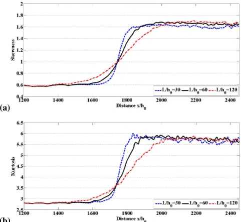
To evaluate the influence of the transitional zone length, we consider three values ofL/h0(Fig. 6), representing steep and smooth depth profiles. The length of the transitional zone does not influence the quantitative parameters (Fig. 7). At large distances from the zone of the depth transformation, the value of kurtosis seems to slightly decay and tends to one of steady state.
4 Wave transformation from shallower to deeper water
An increase of water depth from 5 m to 10 m leads to the attenuation of local wave nonlinearity. Nevertheless, the characteristics of the steady state vary significantly. The deviations from the Gaussian statistics descend appreciably. In particular, kurtosis (Fig. 8b) is close to the values typical for the Gaussian sea state (µ4=3), and the wave asymmetry (Fig. 8a) becomes less pronounced. The comparison of the statistical parameters with the results obtained for the case of constant depth for the same Ursell parameter (see the dashed line in Fig. 8) demonstrates satisfactory agreement for skewness, and some underestimation of kurtosis for the case of constant depth.
(a)
(b)
Fig. 7. Transformation of the skewness (a) and the kurtosis (b) for
different values of transitional zoneL/h0,h0=10 m, Ur = 3.47.
(a)
(b)
(c) c)
Figure 8. Variation of the skewness (a) and kurtosis (b) in the water of variable depth with initial value Ur = 2.06 (dashed line). The same variation in the water of constant depth h0 = 5 m with
Ur = 0.43 (solid line). Variable depth profile with L = 30h0 (c).
Figure 9. The exceedance probability distribution function of wave heights scaled by Hs
corresponded to h=5 m (blue symbols) and h=10 m (red symbols).
5. Conclusion
The transformation of random (irregular) wave fields in the basins of a variable depth is analyzed within the shallow water approximation in the framework of the variable-coefficient Korteweg – de Vries equation. The characteristic amplitude of the surface elevation varies with depth according to Green’s law, what follows from the theoretical model. The skewness and kurtosis are obtained on the basis on numerical simulations. They are shown to grow when the depth decreases (water shallowing), and the wave state deviates from the Gaussian. The probability of the large-amplitude (rogue) waves increases in the transition zone. The characteristics of this process depend on the initial wave steepness (the Ursell parameter), but not on the length of the transitional zone. Obtained results confirm the conclusion made by (Zeng and Trulsen, 2010) in
Fig. 8. Variation of skewness (a) and kurtosis (b) in water of variable depth with initial value Ur = 2.06 (solid line). The same variation in water of constant depthh0=5 m with Ur = 0.43
(dashed line). Variable depth profile withL=30h0(c).
A. Sergeeva et al.: Nonlinear random wave field in shallow water 329
14 Figure 8. Variation of the skewness (a) and kurtosis (b) in the water of variable depth with initial value Ur = 2.06 (dashed line). The same variation in the water of constant depth h0 = 5 m with
Ur = 0.43 (solid line). Variable depth profile with L = 30h0 (c).
Figure 9. The exceedance probability distribution function of wave heights scaled by Hs
corresponded to h=5 m (blue symbols) and h=10 m (red symbols).
5. Conclusion
The transformation of random (irregular) wave fields in the basins of a variable depth is analyzed within the shallow water approximation in the framework of the variable-coefficient Korteweg – de Vries equation. The characteristic amplitude of the surface elevation varies with depth according to Green’s law, what follows from the theoretical model. The skewness and kurtosis are obtained on the basis on numerical simulations. They are shown to grow when the depth decreases (water shallowing), and the wave state deviates from the Gaussian. The probability of the large-amplitude (rogue) waves increases in the transition zone. The characteristics of this process depend on the initial wave steepness (the Ursell parameter), but not on the length of the transitional zone. Obtained results confirm the conclusion made by (Zeng and Trulsen, 2010) in the framework of the nonlinear Schrodinger equation for narrow-banded wind wave field that the
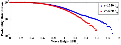
Fig. 9. The exceedance probability distribution function of wave
heights scaled byHs corresponded to h=5 m (blue circles) and
h=10 m (red triangles).
We thus conclude that the probability of extremely high waves decreases when the water becomes deeper, which is demonstrated in Fig. 9, where distribution functions corresponding toh=10 m andh=5 m are presented.
5 Conclusions
The transformation of random (irregular) wave fields in basins of a variable depth is analyzed within the shallow water approximation in the framework of the variable-coefficient Korteweg-de Vries equation. The characteristic amplitude of the surface elevation varies with depth according to Green’s law, which follows the theoretical model. Skewness and kurtosis are obtained on the basis of numerical simulations. They are shown to increase when the depth decreases (water shallowing), and the wave state deviates from the Gaussian. The probability of large-amplitude (rogue) waves increases in the transition zone. The characteristics of this process depend on the initial wave steepness (the Ursell parameter), but not on the length of the transitional zone. The results obtained confirm the conclusion made by Zeng and Trulsen (2010) in the framework of the nonlinear Schrodinger equation for narrow-banded wind wave field, that kurtosis and the number of freak waves may significantly differ from the values expected for a flat bottom of a given depth. The same conclusion was arrived at for the representation of the wave field as a low-density “solitonic gas”; the high-amplitude tail of the distribution function increases more significantly when the water becames shallower. If the waves propagates into a deeper water region, the number of freak waves decreases, and the wave field becames closer to the linear one.
Similar effects are believed to exist for the case of shallow-water internal wave fields described by the extended Korteweg-de Vries equation (Holloway et al., 1997, 1999; Grimshaw et al., 2007). In particular, rogue internal waves are predicted theoretically in the framework of the modified Korteweg-de Vries equation, in which the quadratic nonlinear term equals to zero (Grimshaw et al., 2005), and the Gardner equation has a positive cubic nonlinear term (Grimshaw et al., 2010).
Acknowledgements. The authors would like to acknowledge
partial support from a RFBR grant 09-05-00204, the President grant MK-6734.2010.5, the State Contract No. 02.740.11.0732 and the RAS Programme “Nonlinear Dynamics”. A part of the research was supported by the European Community’s Seventh Framework Programme FP7-SST-2008-RTD-1 under grant agreement No. 234175.
Edited by: C. Kharif
Reviewed by: H. B. Branger and another anonymous referee
References
Didenkulova, I. I., Slunyaev, A. V., Pelinovsky, E. N., and Kharif, C.: Freak waves in 2005, Nat. Hazards Earth Syst. Sci., 6, 1007– 1015, doi:10.5194/nhess-6-1007-2006, 2006.
Didenkulova, I., Pelinovsky, E., and Sergeeva, A.: Runup of long irregular waves on plane beach, in: Extreme Ocean Waves, edited by: Pelinovsky, E. and Kharif, C., Springer, 83–94, 2008. Didenkulova, I., Pelinovsky, E., and Sergeeva, A.: Statistical
characteristics of long waves nearshore, Coast. Eng., 58, 94–102, doi:10.1016/j.coastaleng.2010.08.005, available at:
http://dx.doi.org/10.1016/j.coastaleng.2010.08.005, 2011. Drazin, P.G. and Johnson, R. S.: Solitons: an Introduction,
Cambridge Univ. Press, 1996.
Dysthe, K., Krogstad, H. E., and Muller, P.: Oceanic rogue waves, Annu. Rev. Fluid Mech., 40, 287–310, 2008.
Fornberg, B.: A practical guide to pseudospectral methods, Cambridge University Press, 1998.
Grimshaw, R., Pelinovsky, E., Talipova, T., Ruderman, M., and Erdelyi, R.: Short-lived large-amplitude pulses in the nonlinear long-wave model described by the modified Korteweg-de Vries equation, Stud. Appl. Math., 114(2), 189–210, 2005.
Grimshaw, R., Pelinovsky, E., and Talipova, T.: Modeling internal solitary waves in the coastal ocean, Surv. Geophys., 28(4), 273– 298, 2007.
Grimshaw, R., Pelinovsky, E., Talipova, T., and Sergeeva, A.: Rogue internal waves in the ocean: long wave model, Eur. Phys. J.-Spec. Top., 185, 195–208, 2010.
Holloway, R., Pelinovsky, E., Talipova, T., and Barnes, B.: A nonlinear model of the internal tide transformation on the Australian North West Shelf, J. Phys. Oceanogr., 27(6), 871–896, 1997.
Holloway, P., Pelinovsky, E., and Talipova, T.: A Generalised Korteweg-de Vries model of internal tide transformation in the coastal zone, J. Geophys. Res., 104(C8), 18333–18350, 1999. Huntley, D. A., Guza, R. T., and Bowen, A. J.: A universal form for
shoreline run-up spectra, J. Geophys. Res., 82(18), 2577–2581, 1977.
Janssen, P. A. E. M.: Nonlinear four wave interaction and freak waves, J. Phys. Oceanogr., 33, 863–884, 2003.
Johnson, R. S.: On the development of a solitary wave moving over an uneven bottom, PCPS-P. Camb. Philol. S., 73, 183–203, 1973. Kharif, C., Pelinovsky, E., and Slunyaev, A.: Rogue Waves in the
Ocean, Springer, 2009.
Lavrenov, I.: Wind waves in oceans, Springer-Verlag, 2003. Liu, P. C.: A chronology of freaque wave encounters, Geofizika,
330 A. Sergeeva et al.: Nonlinear random wave field in shallow water
Mori, N. and Janssen, P. A. E. M.: On kurtosis and occurrence probability of freak waves, J. Phys. Oceanogr., 36, 1471–1483, 2006.
Nakoulima, O., Zahibo, N., Pelinovsky, E., Talipova, T., and Kurkin, A.: Solitary wave dynamics in shallow water over pe-riodic topography, Chaos, 15, 037107, doi:10.1063/1.1984492, 2005.
Novikov, S., Manakov, S. V., Pitaevskii, L. P., and Zakharov, V. E.: Theory of Solitons: the Inverse Scattering Method, Consultants Bureau, New York, 1984.
Onorato, M., Osborne, A. R., Serio, M., Cavaleri, L., Brandini, C., and Stansberg, C. T.: Extreme waves, modulational instability and second-order theory: wave flume experiments on irregular waves, Eur. J. Mech. B-Fluid., 25, 586–601, 2006.
Ostrovsky, L. A. and Pelinovsky, E. N.: Wave transformation of the surface of a fluid of variable depth, Izvestiya, Atmos. Oceanic Phys., 6(9), 552–555, 1970.
Pelinovsky, E. N.: On the soliton evolution in inhomogeneous media, Applied Mechanics and Technical Physics, 6, 80–85, 1971.
Pelinovsky, E. and Sergeeva (Kokorina), A.: Numerical modeling of the KdV random wave field, Eur. J. Mech. B-Fluid., 25, 425– 434, 2006.
Salupere, A., Maugin, G. A., Engelbrecht, J., and Kalda, J.: On the KdV soliton formation and discrete spectral analysis, Wave Motion, 123, 49–66, 1996.
Salupere, A., Peterson, P., and Engelbrecht, J: Long-time behaviour of soliton ensembles. Part 1 – Emergence of ensembles, Chaos Soliton. Fract., 14, 1413–1424, 2002.
Salupere, A., Peterson, P., and Engelbrecht, J.: Long-time behaviour of soliton ensembles. Part 2 – Periodical patterns of trajectories, Chaos Soliton. Fract., 15, 29–40, 2003a.
Salupere, A., Peterson, P., and Engelbrecht, J.: Long-time behavior of soliton ensembles, Math. Comput. Simulat., 62, 137–147, 2003b.
Shemer, L. and Sergeeva, A.: An experimental study of spatial evolution of statistical parameters in a unidirectional narrow-banded random wave field, J. Geophys. Res., 114, C01015, doi:10.1029/2008JC005077, 2009.
Shemer, L., Sergeeva, A., and Slunyaev, A.: Applicability of envelope model equations for simulation of narrow-spectrum unidirectional random field evolution: experimental validation, Phys. Fluids, 22, 016601, 1–9, doi:10.1063/1.3290240, 2010. Tappert, F. D. and Zabusky, N. J.: Gradient-induced fission of
solitons, Phys. Rev. Lett., 27, 1774–1776, 1971.
Zakharov, V. E.: Kinetic equation for solitons, Soviet JETP, 60, 993–1000, 1971.