Causal Modeling Under Complex Dependency in Clustered and Longitudinal Observations

University of Pennsylvania

ScholarlyCommons

Publicly Accessible Penn Dissertations

1-1-2014

Causal Modeling Under Complex Dependency in

Clustered and Longitudinal Observations

Jiwei He

University of Pennsylvania, [email protected]

Follow this and additional works at:

http://repository.upenn.edu/edissertations

Part of the

Biostatistics Commons

This paper is posted at ScholarlyCommons.http://repository.upenn.edu/edissertations/1311

Recommended Citation

He, Jiwei, "Causal Modeling Under Complex Dependency in Clustered and Longitudinal Observations" (2014).Publicly Accessible

Penn Dissertations. 1311.

Causal Modeling Under Complex Dependency in Clustered and

Longitudinal Observations

Abstract

In assessing the efficacy of a time-varying treatment Marginal Structural Models (MSMs) and Structural

Nested Mean Models (SNMMs) are useful in dealing with confounding by variables affected by earlier

treatments. MSMs model the joint effect of treatments on the marginal mean of the potential outcome,

whereas SNMMs model the joint effect of treatments on the mean of the potential outcome conditional on

the treatment and covariate history. These models often consider independent subjects with noninformative

time of observation.

The first two chapters extend the two classes of models to clustered observations with time-varying treatments

in the presence of time-varying confounding. We formulate models with both cluster- and unit-level

treatments and derive semiparametric estimators of parameters in such models. For unit-level treatments, we

consider both the presence and absence of interference, namely the effect of treatment on outcomes in other

units of the same cluster. For MSMs, we show that the use of unit-specific inverse probability weights and

certain working correlation structures can improve the efficiency of estimators under specified conditions.

The properties of the estimators are evaluated through simulations and compared with the conventional GEE

regression method for clustered outcomes. To illustrate our methods, we use data from the treatment arm of a

glaucoma clinical trial to compare the effectiveness of two commonly used ocular hypertension medications.

The third chapter extends SNMMs to situations with intermittent missing observations. In observational

longitudinal studies, subjects often miss prescheduled visits intermittently. Previous literature has mainly

focused on dealing with monotone censoring due to early dropout. Here we focus on intermittent missingness

that can depend on the subjects' covariate and treatment history. We show that under certain assumptions the

standard SNMMs can be used for situations where non-outcome covariates are missing intermittently. In

situations where outcomes are also missing intermittently, we use a method that does not require artificially

censoring the data, but requires a strict missing at random assumption. The estimators are shown to be

consistent and achieve reasonable efficiency. We illustrate the method by estimating the effect of non-steroidal

anti-inflammatory drugs (NSAIDs) on genitourinary pain using data from a study of chronic pelvic pain.

Degree Type

Dissertation

Degree Name

Doctor of Philosophy (PhD)

Graduate Group

Epidemiology & Biostatistics

Keywords

Causal Inference, Clustered data, Longitudinal data, Structural models

CAUSAL MODELING UNDER COMPLEX DEPENDENCY IN CLUSTERED AND LONGITUDINAL OBSERVATIONS

Jiwei He

A DISSERTATION

in

Epidemiology and Biostatistics

Presented to the Faculties of the University of Pennsylvania

in

Partial Fulfillment of the Requirements for the

Degree of Doctor of Philosophy

2014

Supervisor of Dissertation

Alisa J. Stephens

Assistant Professor of Biostatistics

Graduate Group Chairperson

John H. Holmes, Associate Professor of Medical Informatics in Epidemiology

Dissertation Committee

Russell Taki Shinohara, Assistant Professor of Biostatistics

John H. Kempen, Professor of Ophthalmology

CAUSAL MODELING UNDER COMPLEX DEPENDENCY IN CLUSTERED AND

LONGITUDINAL OBSERVATIONS

c

COPYRIGHT

2014

Jiwei He

This work is licensed under the

Creative Commons Attribution

NonCommercial-ShareAlike 3.0

License

To view a copy of this license, visit

ACKNOWLEDGEMENT

I would like to thank my advisor, Dr. Marshall Joffe, for his mentorship, guidance and support

throughout my dissertation. He is a knowledgeable, patient and inspiring mentor. He introduced

me to the area of causal inference and helped me make progress in my dissertation until he was

forced to take medical leave. I really appreciate his efforts to offer suggestions to my work and

presentations at a challenging time. I would also like to thank my co-advisor Dr. Alisa Stephens,

who kindly agreed to supervise me when Marshall was on leave. She helped me frame the last

chapter of my dissertation and dedicated a lot of time revising my entire dissertation. This work

would not have been possible without them. I am grateful to other members of my committee,

Drs. Taki Shinohara, John Kempen and Linda Zhao for their feedback and encouragement in my

dissertation work, and Dr John Kempen for also providing expertise in ophthalmology. I would also

llike to thank Dr. Jason Roy for checking on my progress and offering valuable suggestions and Dr.

Justine shults for her guidance in my master’s thesis and encouragement throughout my time in the

program.

I would like to thank our graduate group chairs, Drs. Mary Putt and Daniel Heitjan, for assigning

me with interesting research assistant projects. I am grateful that I had the opportunity to explore a

variety of research topics outside my dissertation area and also gain some consulting experience.

I would also like to thank Drs. Wei-Ting Hwang, Pamela Shaw, Richard Entsuah for supervising me

on these projects as well as clinical collaborators Drs. John Christoduleas and Brian Baumann for

their expertise and guidance in medical research.

I further need to thank all of the faculty and staff of the Department of Biostatistics and

Epidemi-ology. I have learned a lot from their classes, and I would not have been able to complete my

dissertation without those skills. I also need to thank my parents for their love and support for

many years. I would like to thank Drs. Minghong Ma and Johnathan Raper in the Department of

Neuroscience for their support when I changed my major to biostatistics. I would also like to thank

my fellow students in the program especially those from the same cohort as well as my roommates

ABSTRACT

CAUSAL MODELING UNDER COMPLEX DEPENDENCY IN CLUSTERED AND

LONGITUDINAL OBSERVATIONS

Jiwei He

Alisa J. Stephens

In assessing the efficacy of a time-varying treatment Marginal Structural Models (MSMs) and

Struc-tural Nested Mean Models (SNMMs) are useful in dealing with confounding by variables affected by

earlier treatments. MSMs model the joint effect of treatments on the marginal mean of the potential

outcome, whereas SNMMs model the joint effect of treatments on the mean of the potential

out-come conditional on the treatment and covariate history. These models often consider independent

subjects with noninformative time of observation.

The first two chapters extend the two classes of models to clustered observations with time-varying

treatments in the presence of time-varying confounding. We formulate models with both

cluster-and unit-level treatments cluster-and derive semiparametric estimators of parameters in such models. For

unit-level treatments, we consider both the presence and absence of interference, namely the effect

of treatment on outcomes in other units of the same cluster. For MSMs, we show that the use of

unit-specific inverse probability weights and certain working correlation structures can improve the

efficiency of estimators under specified conditions. The properties of the estimators are evaluated

through simulations and compared with the conventional GEE regression method for clustered

outcomes. To illustrate our methods, we use data from the treatment arm of a glaucoma clinical

trial to compare the effectiveness of two commonly used ocular hypertension medications.

The third chapter extends SNMMs to situations with intermittent missing observations. In

observa-tional longitudinal studies, subjects often miss prescheduled visits intermittently. Previous literature

has mainly focused on dealing with monotone censoring due to early dropout. Here we focus on

in-termittent missingness that can depend on the subjects’ covariate and treatment history. We show

that under certain assumptions the standard SNMMs can be used for situations where non-outcome

covariates are missing intermittently. In situations where outcomes are also missing intermittently,

random assumption. The estimators are shown to be consistent and achieve reasonable efficiency.

We illustrate the method by estimating the effect of non-steroidal anti-inflammatory drugs (NSAIDs)

TABLE OF CONTENTS

ACKNOWLEDGEMENT . . . iii

ABSTRACT . . . iv

LIST OF TABLES . . . ix

LIST OF ILLUSTRATIONS . . . x

CHAPTER 1 : INTRODUCTION . . . 1

1.1 Background . . . 1

1.2 Novel Developments . . . 2

CHAPTER 2 : STRUCTURAL NESTED MEAN MODELS TO ESTIMATE THE EFFECTS OF TIME -VARYING TREATMENTS ON CLUSTERED OUTCOMES . . . 4

2.1 Introduction . . . 4

2.2 Notation for clustered observations . . . 5

2.3 Structural models and estimation for point treatments in clustered observations . . . 6

2.4 Structural models and estimation for time-varying treatments in clustered observations 12 2.5 Simulation study . . . 16

2.6 Analysis of glaucoma data . . . 20

2.7 Discussion . . . 22

CHAPTER 3 : MARGINAL STRUCTURAL MEAN MODELS TO ESTIMATE THE EFFECTS OF TIME -VARYING TREATMENTS ON CLUSTERED OUTCOMES . . . 26

3.1 Introduction . . . 26

3.2 Notation for clustered observations . . . 27

3.3 Marginal structural models and estimation for a point treatment in clustered observa-tions . . . 28

3.4 Marginal structural models and estimation for time-varying treatments in clustered observations . . . 32

3.6 Analysis of glaucoma study . . . 40

3.7 Discussion . . . 42

CHAPTER 4 : ESTIMATION OF STRUCTURAL NESTED MEAN MODELS IN LONGITUDINAL STUD -IES WITH INTERMITTENT MISSING OBSERVATIONS . . . 46

4.1 Introduction . . . 46

4.2 Longitudinal data with intermittent missing observations . . . 47

4.3 Intermittent missingness in non-outcome covariates . . . 48

4.4 Intermittent missingness in outcomes . . . 53

4.5 Analysis of MAPP data . . . 57

4.6 Discussion . . . 60

CHAPTER 5 : DISCUSSION. . . 62

5.1 Future directions . . . 63

APPENDICES . . . 66

LIST OF TABLES

TABLE 2.1 : Small and large sample performance of g-estimators in a simulation study based onExample 1. DR1 estimator and DR2 estimator are dou-bly robust, whereas non-DR estimator is not. DR1 uses a flexible working model for the covariance, whereas DR2 estimator assumes independence and constant variance over time. AVE EST refers to average estimates, EMP SE refers to empirical standard error, AVE SE refers to average asymptotic standard error, and REL√MSErefers to square root of mean squared error. 24 TABLE 2.2 : Estimates for variance parameterσ2

m and correlation parameterρm at

each time point for DR1 estimator fromExample 1.Sample size N=1000.

σ2

mandρmare estimated by the method of moments approach by Liang and Zeger (1986). AVE EST refers to average estimates, and EMP SE refers to empirical standard error. . . 25 TABLE 2.3 : Compare the estimators obtained from SNMM and g-estimation to those

from GEE linear regression using two simulation examples. Sample size N=1000. InExample 1, the association between covariates and poten-tial outcomes is linear, whereas inExample 2, the association is quadratic. EMP SE refers to empirical standard error, and√MSErefers to square root of mean squared error. . . 25 TABLE 2.4 : Results of glaucoma data analysis. Estimators from doubly robust (DR)

and non-doubly robust (non-DR) approaches are shown. EST refers to esti-mate, and SE refers to asymptotic standard error. . . 25

TABLE 3.1 : Combination of weights and working correlations required for obtain-ing consistent estimator under different conditions. . . . 35 TABLE 3.2 : Compare estimators obtained from MSM to those from standard GEE

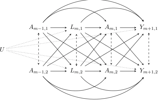
regression. Sample size N=1000. ψ0 represents the intercept, ψ1 rep-resents the effect of treatment on the same unit, ψ2 represents the effect of treatment on the opposite unit,ψ3 represents interaction between treat-ments. The true values of parameters areψ0= 0, ψ1= 2, ψ2 = 1, ψ3= 0.5. Independence working correlation was used for units and between-times correlation. . . 44 TABLE 3.3 : Compare estimators from MSM with different working correlations for

the example with interference. Sample size N=1000. ψ0 represents the intercept,ψ1represents the effect of treatment on the same unit,ψ2 repre-sents the effect of treatment on the opposite unit,ψ3represents interaction between treatments. The true values of parameters areψ0= 0, ψ1= 2, ψ2=

1, ψ3 = 0.5. The weights used are cluster-specific. The weights used for AR(1) between times correlation are also time-fixed. . . 45 TABLE 3.4 : Compare estimators from MSM with different working correlations for

TABLE 3.5 : Analysis of results from glaucoma study using GEE, MSM with un-stabilized and un-stabilized IPW respectively. ψ0 represents the intercept,

ψ1 represents the effect of beta-blocker only on the same unit, ψ2 repre-sents the difference between prostaglandin analogue and beta blocker on the same unit, ψ3 represents the difference between combined treatment and beta blocker on the same unit. The weights used are time-specific and unit-specific. . . 45

TABLE 4.1 : Results for the example with intermittent missingness in non-outcome covariates. Average estimates (EST), empirical standard errors (SE), av-erage asymptotic standard errors (ASE) and95% coverage probability are listed for the correctly specified treatment as well as the mis-specified treat-ment model that omitsCm−1. . . 53 TABLE 4.2 : Results for the example with intermittent missingness in covariates

and outcome. Average estimates (EST), empirical standard errors (SE), average asymptotic standard errors (ASE) and95%coverage probability are listed for unweighted estimating equation (No IPW), our approach with un-stabilized (IPW) or un-stabilized (Stabilized IPW) weights, monotone censoring approach with unstabilized (Monotone IPW) or stabilized (Monotone stabi-lized IPW) weights withK= 5orK= 7. . . 58 TABLE 4.3 : Results for the example with intermittent missingness in covariates

and outcome, in which if weights are greater than 200, they are trun-cated at 200. . . . 58 TABLE 4.4 : Results from analyzing MAPP data . . . 60

TABLE B.1 : Compare estimators from MSM with different working correlations for the example with interference. Sample size N=1000. ψ0 represents the intercept,ψ1represents the effect of treatment on the same unit,ψ2 repre-sents the effect of treatment on the opposite unit,ψ3represents interaction between treatments. The true values of parameters areψ0= 0, ψ1= 2, ψ2=

1, ψ3 = 0.5. The weights used are cluster-specific. The weights used for AR(1) between times correlation are also time-fixed. . . 74 TABLE B.2 : Compare estimators from MSM with different working correlations for

LIST OF ILLUSTRATIONS

FIGURE 2.1 : DAG for an example with single time point . . . 7

FIGURE 2.2 : Partial DAG for an example with time-varying treatments . . . 12

FIGURE 3.1 : Directed acyclic graph (DAG) for a single time point example. . . 28

FIGURE 3.2 : Partial DAG for an example with time-varying treatments. . . 32

FIGURE 4.1 : Confounding due to missing indicator Scenario 1 . . . 50

FIGURE 4.2 : Confounding due to missing indicator Scenario 2 . . . 50

CHAPTER 1

I

1.1. Background

In assessing the efficacy of a time-varying treatment Marginal Structural Models (MSMs) and

Struc-tural Nested Models (SNMs) are useful in dealing with confounding by variables affected by earlier

treatments. MSMs model the joint effects of treatment on the marginal mean of the potential

out-come. There are two types of SNMs: (1) structural nested mean models (SNMMs) model the joint

effect of treatment on the mean of the outcome conditional on the treatment and covariate history,

and (2) structural nested distribution models (SNDMs) model the joint effect of treatment on the

entire distribution of the outcome conditional on the treatment and covariate history. Compared to

MSMs, SNMs have the advantage of being able to model effect modification by time-varying

co-variates, whereas MSMs can only model effect modification by baseline covariates. SNMs are also

useful for modeling the effect of dynamic treatment regimes, in which the treatment plan changes

according to observed patient characteristics during the treatment course, in contrast to static

treat-ment regimes, in which the entire treattreat-ment schedule is known at the time of initiation. Another

advantage of SNMs is that they can work under conditions where certain assumptions fail. For

ex-ample, SNMs may be fit under instrumental variable assumptions when there is unmeasured

con-founding. Despite these advantages of SNMs, MSMs are more widely used compared to SNMs,

partly because the models are easier to understand and can be implemented with standard

soft-ware.

SNMs and MSMs often consider treatment allocation and repeated measures at the individual

level. These models have seldom been used for clustered observations. A common example for

clustered outcomes is eye disease treatment, where two eyes of a given subject form a cluster.

Other examples include infectious diseases among members of the same household etc. Rubin

(1986) calls a situation where “the observation on one unit is unaffected by the particular treatment

assignment to the other units” the “stable unit-treatment value assumption (SUTVA)” [19]. If we

consider each eye as a separate unit for treatment, the SUTVA assumption may be violated. Under

the same subject. If the treatments are binary, each eye will have not only two but four possible

treatments, depending on the treatment received by both eyes. VanderWeele (2008) has discussed

SUTVA in the context of neighborhood effects [26]. To our knowledge, the only published work in

this category is from Brumback et al. (2014), where SNMs and an instrumental variable approach

were used to estimate the effect of cluster-level treatment on unit-level outcomes in the presence

of unmeasured confounding [1].

In observational longitudinal studies, subjects are often observed at random times with

subject-specific intervals between consecutive visits. A conventional approach is to convert continuous

time to discrete time points. This will result in intermittent missing observations for many subjects.

In other cases, subjects may miss prescheduled visits intermittently depending on their condition

throughout the study. Most of the previous literature focuses on dealing with monotone censoring.

One approach to analyzing intermittent missing data is to artificially censor the data as

mono-tone and use methods appropriate for monomono-tone data [10]. However, this approach will result in

significant loss of information, especially if many subjects miss an early visit but later return. Time

varying treatments and dynamic observation schedules have been considered with regard to MSMs

by Hern´an et al. (2009) [6]. Most of their work is based on the assumption that treatment changes only occur at observed times. They used inverse probability weighting to adjust for selection bias

due to the missing outcomes. We consider the implications of dynamic treatment schedules for

es-timating parameters in SNMMs. Like Herna´n et al. (2009), we will focus on the setting of dynamic observation plan, where a subject’s observation times depend on his treatment and covariate

his-tory.

1.2. Novel Developments

In this dissertation, we develop statistical methods for the design and analysis of longitudinal

ob-servational data with clustered observations or intermittent missing observations. The dissertation

consists of three parts. In Chapter 2, we extend SNMMs to clustered observations with time-varying

confounding and treatments. This is a generalization of Brumback et al. (2014)’s method [1]. We

demonstrate how to formulate models with both cluster- and unit-level treatments and show how

to derive semiparametric estimators of parameters in such models. For unit-level treatments, we

The properties of the estimators are evaluated through simulations and compared with the

conven-tional GEE regression method for clustered outcomes. To illustrate our methods, we use data from

the treatment arm of a glaucoma clinical trial to compare the effectiveness of two commonly used

ocular hypertension medications.

In Chapter 3, we extend MSMs to clustered observations with time-varying confounding and

treat-ments. Again we demonstrate how to formulate models with both cluster- and unit-level treatments

and show how to derive semiparametric estimators of parameters in such models. We consider

cases where there is presence or absence of interference. We also consider using unit-specific

inverse probability weights (IPWs) and certain working correlation structures to improve the

effi-ciency of estimators under specified conditions. We use the same glaucoma clinical trial data for

illustration and compare the results from the SNMM approach.

In Chapter 4, we extend SNMMs to situations with intermittent missing observations. We show

that under assumptions of last observation carried forward treatment and ignorable treatment the

regular SNMMs can be used for situations where non-outcome covariates are missing intermittently.

We further consider intermittently missing outcomes and use an inverse probability of weighting

approach. Whereas missing data methods often censor subjects after the first missed visit, we

used a method that does not require artificially censoring the data, but requires a stricter MAR

assumption. Results from our simulation studies show that the estimators are consistent and show

some advantage in efficiency in comparison to the monotone censoring approach. To illustrate our

method, we use data from a study of chronic pelvic pain to estimate the effect of non-steroidal

CHAPTER 2

S

TIME

-

2.1. Introduction

Structural nested models (SNMs) are a class of models that is useful for estimating the causal

ef-fect of a time-varying treatment in the presence of time-varying confounding [12]. In some studies,

treatments are affected by covariates at earlier time points and subsequently affect covariates at

later time points. Confounding that arises in such situations cannot be properly controlled for by

conventional regression methods. However, such problems can be solved by several other

meth-ods, including marginal structural models (MSMs) and SNMs. Compared to MSMs, SNMs have the

advantage of being able to model effect modification by time-varying covariates, whereas MSMs

can only model effect modification by baseline covariates. SNMs are also useful for modeling the

effect of dynamic treatment regimes, in which the treatment plan changes according to observed

patient characteristics during the treatment course, in addition to static treatment regimes, in which

the entire treatment schedule is known at the time of initiation. Another advantage of SNMs is that

they can work under conditions where certain assumptions fail. For example, SNMs may be fit

un-der instrumental variable assumptions when there is no unmeasured confounding. There are two

types of SNMs: (1) structural nested mean models (SNMMs) model the joint effect of treatments

on the mean of the outcome conditional on the treatment and covariate history, and (2) structural

nested distribution models (SNDMs) model the joint effect of treatments on the entire distribution of

the outcome conditional on the treatment and covariate history. So far, SNMs have seldom been

used for clustered observations. Brumback et al. (2014) used SNMs and an instrumental variable

approach to estimate the effect of cluster-level treatment on unit-level outcomes in the presence

of unmeasured confounding [1]. This paper generalizes previous work by formulating SNMMs for

clustered observations with time-varying confounding and treatments. The formulation applies to

both unit-level and cluster-level treatments.

A motivating example is the study of eye disease treatment, where two eyes of a given subject form

subject-specific characteristics. Rubin (1986) calls a situation where “the observation on one unit

is unaffected by the particular treatment assignment to the other units” the “stable unit-treatment

value assumption (SUTVA)” [19]. If we consider each eye as a separate unit for treatment, the

SUTVA assumption may be violated. Under eye-specific treatment, treatment received by one

eye may affect outcomes in the other eye of the same subject. If the treatments are binary, each

eye will have not only two but four possible treatments, depending on the treatment received by

both eyes. VanderWeele (2008) has discussed the SUTVA in the context of neighborhood effects

[26]. In the ophthalmology study, treatments are eye-specific drops. Treatments, clinical covariates,

and outcomes are measured repeatedly over an extended period of time; treatments are therefore

subject to time-dependent confounding. We are interested in modeling the joint effect of a series

of treatments on a series of clustered outcomes. Other examples of clustered observations include

repeated measurements of disease symptoms on the same individual or an infectious disease

among people in the same household.

The structure of the paper is as the following: we first describe the setup for exploring causal effects

among clustered observations. We then formulate SNMMs for clustered observations in a single

time point setting and describe an efficient estimating equation. We then extend the model and

estimation to time-varying treatments and repeatedly measured outcomes. Last, the method is

evaluated using simulation studies and applied to an ophthalmology dataset.

2.2. Notation for clustered observations

We first describe the general structure of data with repeatedly measured treatments and repeatedly

measured clustered outcomes and the definition of a causal effect in such a context. The notation

is based on Robins (1994) with extension for clustered data [12]. Suppose that data is collected on

N clusters,i= 1,2, ..., N atK+ 1time points,k= 0,1, ..., K. At each time pointk, outcomes are measured fromJ units in each cluster,j= 1,2, ..., J. LetAimjdenote unit-specific treatment in the

jth unit at timemfor clusteri, andA†_imdenote systemic treatment received at timemfor clusteri. LetLijmdenote unit-specific covariates in thejth unit, andL†imdenote cluster-specific covariates measured at timemfor clusteri.Yimjdenotes the observed outcome injth unit measured at time

clusteri.Yim={Yim1, ..., YimJ}is all observed outcomes measured at timemin clusteri. We use overbars to denote the history of a variable; thus, A¯im ={Ai0,Ai1, ...,Aim} is treatment history through timem in cluster i, and L¯im = {Li0,Li1, ...,Lim} is covariate history through time min clusteri. We use underbars to denote the future of a variable; thus,Y_i,m={Yi,m,Yi,m+1, ...,Yi,K} is outcomes observed since timemin clusteri. If unstated, the notation in formulation and figures is for one cluster and therefore omits the subscriptifor cluster. The subscriptmfor time is omitted in examples with single time point. UnboldAim, Lim, Yimrepresent scalar treatment, covariate and outcome, respectively for subjecti at timem in situations without clustered outcomes, which we use to reference previous literature on SNMMs.

To define causal effects and structural models, we will use potential or counterfactual outcomes

that are outcomes that would be observed were the subject to receive a certain treatment [20]. We

presume that treatments at timemdo not affect outcomes prior to timem. Potential outcomes are considered under a regime, which is defined as a sequential set of treatments¯aK ={a1, ...,aK}. In formulating SNMs, the regime(¯am,0), the counterfactual treatment regime that agrees witha¯m through timemand is0thereafter, is of particular interest. LetY¯am,0

i,k =

n

Ya¯m,0

ik1 , ..., Y ¯ am,0

ikJ

o

denote

the potential outcome in clusterithat would be observed at timekwherek > mwere the cluster to receive treatment historya¯mthrough timemand0thereafter. LetY¯ai,m+1m,0 ={Y

¯ am,0

i,m+1, ...,Y ¯ am,0

i,K }

denote the series of potential outcomes in clusterithat would be observed after timem. Causal effects can be defined as contrasts of potential outcomes for the same group of subjects under

different treatment regimes. For instance,Y¯aK

i,m−Y ¯ a0

K

i,m, where¯aK 6= ¯a0K, denotes the causal effect of treatment¯aK versus¯a0K on a subject’s outcome at timem.

2.3. Structural models and estimation for point treatments in clustered

observa-tions

Prior to describing the formulation of SNMMs for clustered observations, we review the general

concepts of SNMMs for nonclustered outcomes. SNMMs model the contrast between conditional

means of potential outcomesγ_m∗(¯lm,¯am) =g

EY¯am,0

m+1|L¯m= ¯lm,A¯m= ¯am

−

gEYa¯m−1,0

m+1 |L¯m= ¯lm,A¯m= ¯am

the means of subsequent potential outcomes after having removed the effect of all later treatments,

a process called “blipping down” [12]. A functionγ∗

m(¯lm,¯am)that defines such a contrast is called a blip function. It can be parameterized with finite dimensional parameterψ.

We first formulate SNMMs for clustered outcomes in a single time point example, where treatments,

covariates and outcomes are measured at one time point only. In this example, we assume that

each cluster consists of two units, and consider unit-level treatment only. The results can be easily

generalized to situations with more than two units or with cluster-level treatment. A directed acyclic

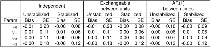
graph (DAG) is shown in Figure 2.1. The subscript here refers to unit number. L={L1, L2, L†}is the set of cluster- and unit-level measured confounder for the effect of joint treatmentA={A1, A2} on clustered outcomesY = {Y1, Y2}. We assume that there is no unmeasured confounding be-tweenAandY. Dashed double arrows represent possible unmeasured confounding withinL,Aor

Ybetween units.Uand dotted arrows represent possible unmeasured confounding betweenLand

Y. LetYa

j =Y

aj,aj0

j denote the potential outcome injth unit, whereaj andaj0 refer to unit-specific

treatment to the same unit and the other within-cluster unit respectively,{j, j0}={1,2},{2,1}.

L†

L1

L2

A1

A2

Y1

Y2

U

Figure 2.1: DAG for an example with single time point

2.3.1. Structural nested mean models

a contrast between means of potential outcomes under joint treatment versus means of potential

outcomes under no treatment as seen in (1). If there is an additional binary systemic treatmentA†_,

the combined treatment{A†, A1, A2}will contain8levels.

E



 

Ya1,a2

1

Ya2,a1

2

L=l,A=a 

 −E



 

Y₁0,0 Y₂0,0

L=l,A=a 

 =



 

γ₁∗(a1, a2,l)

γ₂∗(a2, a1,l)





. (2.1)

The vector-valued blip functionγ∗(.)models the effect of removing joint treatmentafrom both unit-level outcomes within the cluster. It can be parameterized with the finite dimensional parameterψ

to form



 

γ∗₁(a1, a2,l;ψ)

γ∗2(a2, a1,l;ψ)





. (2.2)

As an example, let



 

γ₁∗(a1, a2, l;ψ)

γ₂∗(a2, a1, l;ψ)



 =



 

ψ1a1+ψ2a2+ψ3a1a2

ψ10a₂+ψ₂0a₁+ψ₃0a₂a₁





. (2.3)

In (2.3), ψ ∈ R6_{; ψ}

1 andψ10 represent the effect of unit-specific treatment on the outcome in the

same unit, ψ2 andψ20 represent the effect of treatment on the outcome in the opposite unit, ψ₃

andψ30 represent the interaction between treatments in different units. This example imposes the

assumption that effect modification by covariates is absent.

The dimension of causal parameters will increase sharply with increase in the number of units per

cluster. Some additional model assumptions are considered to reduce the dimension of causal

parameters. For the ophthalmology example, it is reasonable to assume symmetry between two

eyes, namely the effect of the joint treatment is the same for each unit. In (2.3), the symmetry

assumption implies ψ1 = ψ10, ψ₂ = ψ₂0, ψ₃ = ψ₃0. In some cases, we may want to assume no

interference, namely unit-specific treatment on one unit has no effect on outcomes in the other

units of the same cluster. With two units per cluster, it refers to

Yaj,aj0

j =Y

aj,0

In (2.3), the no interference assumption impliesψ2=ψ3=ψ20 =ψ₃0 = 0.

2.3.2. Identifiability

A1-A3 below are sufficient assumptions to identify the causal effect of joint treatmentarelative to

no treatment from observed data and therefore the causal parameterψ. A1. Consistency. IfA=afor a given cluster, thenYa_{=Yfor that cluster.}

A2. Conditional exchangeability. Y0,0_⊥A|L=l.

A3. Positivity. IffL(l)>0, thenfA|L(a|l)>0for all treatmentsa.

In the presence of interference between units, potential outcomes like Yaj

j are not well-defined.

However, under no interference, it is reasonable to relax A1 and define consistency under the

standard assumption for non-clustered data: ifAj = aj for a given unit j, thenY aj

j = Yj for that unit. A3 can be relaxed in SNMMs such that the assumption does not need to hold for allLwith

fL(l)>0.

2.3.3. Alternative modeling

An alternative way of modeling the joint effect of{a1, a2} is to use the concepts in SNMMs with time-varying treatments and sequentially remove the effect of each unit-specific treatment. In the

following example, the effect of treatment on the opposite unit is removed first, followed by the effect

of treatment on the same unit.

1. Remove the effect of treatment on the opposite unitaj0:

EYaj,aj0

j |L=l,A=a

−EYaj,0

j |L=l,A=a

=γ_1,j∗ (aj0,l, a_j) (2.4a)

2. Remove the effect of treatment on the same unitaj:

EYaj,0

j |L=l, Aj=aj

−EY_j0,0|L=l, Aj=aj

For example, the blip functions in (2.4a) and (2.4b) can be parameterized as γ∗_1,j(aj0, l, a_j;ψ) =

ψ2aj0+ψ₃a_j0a_jandγ_2,j∗ (a_j,l;ψ) =ψ₁a_j respectively.

Assumptions A1 and A3 plus a sequential ignorability assumption are sufficient to identify the

causal effect in (2.4a) and (2.4b). Specifically, the sequential ignorability assumption states that

Yaj,0

j ⊥ Aj0|L, A_j andY_j0,0 ⊥ A_j|L. Testing for no interference under this model is equivalent to

testing whether the blip function in (2.4a) equals 0. Since the entire covariate history for the

clus-ter is conditioned on in the sequential blipping down, this approach will not cause any additional

collapsibility problem under logit link, if the sequential ignorability assumption holds; otherwise

re-peated averaging overAj0 is required. However, sincea_janda_j0 are simultaneous treatments, the

order of blipping down is arbitrary. Parameters from different orders of blipping down have different

interpretations. For this reason, the approach in (2.1) is used for the rest of the paper.

2.3.4. Estimation

Robins (1994) has derived a class of estimating equations for parameters of SNMMs based on

semiparametric theory [12]. He defined Hk(ψ) = Yk −Pk_l=0−1γl,k∗ L¯l,A¯l;ψ as the fully blipped down outcome at timek, and H(m) _{= [H}

m+1(ψ), Hm+2(ψ), ...., HK(ψ)]T as the vector of blipped down outcomes after timem, wherem= 0, ..., K−1. Under the sequential ignorability assumption,

E H(m)|L¯m,A¯m

=E H(m)|L¯m,A¯m−1

.H˙(m)is defined asH˙(m)=H(m)−E H(m)|L¯m,A¯m−1

.

The efficient estimating function, known as the efficient score [25], under general settings involves

complex recursive expressions, but under the assumption that

E HkHj|L¯m,A¯m

=E HkHj|L¯m,A¯m−1

, (2.5)

fork > m, j > m, m= 0, ..., K−1, the efficient score can be simplified as:

S_ψef f =

N

X

i=1 K−1

X

m=0

"

E

(

∂H˙_i(m) ∂ψT

¯

Lim,A¯im

)

−E

(

∂H˙_i(m) ∂ψT

¯

Lim,A¯i,m−1

)#

·V arH˙_i(m)|L¯im,A¯i,m−1

−1

·H˙_i(m)

(2.6)

By setting (2.6) to 0 and solving the estimating equation, one can obtain an efficient estimator for

(2.6)in terms of the partially blipped down outcomeUmwith removal of the effect of treatments from time monwards [27]. Specifically, Um is a vector with elementsUm,k = Yk −P

k−1

l=mγl,k∗ L¯l,A¯l

,

for k = m+ 1, ..., K. Um mimics the potential outcomes in the sense that E Um|Lm, Am

=

EYam−1,0

m+1 |Lm, Am

. The alternative expression is:

S_ψef f =

N

X

i=1 K−1

X m=0 E ∂Uim ∂ψT ¯

Lim,A¯im

−E ∂Uim ∂ψT ¯

Lim,A¯i,m−1

·V ar Uim|L¯im,A¯i,m−1)

−1

·

Uim−E Uim|L¯im,A¯i,m−1 (2.7)

The theory for SNMMs can be directly applied to situations with clustered observations. We first

construct blipped down outcomesU. For a single time point example with bivariate outcomes, they

can be written as

U=    Y1 Y2   −   

γ₁∗(A1, A2,L;ψ)

γ₂∗(A2, A1,L;ψ)



 .

The following is a parameterized example for blip function under the symmetry assumption:



 

γ₁∗(a1, a2,l;ψ)

γ₂∗(a2, a1,l;ψ)

  =   

ψ1a1+ψ2a2+ψ3a1a2

ψ1a2+ψ2a1+ψ3a2a1





 (2.8)

Based on (2.7), the efficient score for a single time point example can be written as

S_ψef f =

N

X

i=1

_∂U

i

∂ψT −E

_∂U i ∂ψT Li

·V ar(Ui|Li)−1· {Ui−E(Ui|Li)}. (2.9)

For the example in (2.8), ∂U

∂ψT has the following expression:

∂U

∂ψT =

     

A1 A2

A2 A1

A1A2 A2A1

      .

E_∂ψ∂UT|L

is based on a model for treatment. If treatment probabilities are unknown, a multinomial

joint treatment. The estimating equation in (2.9) is doubly robust, because the estimator forψwill be consistent if either the model forE∂U

∂ψT|L

or the model forE(U|L)is correctly specified. When both are correctly specified and the conditional varianceV ar(U|L)is also correctly specified, the estimator achieves the semiparametric efficiency bound for model (2.2) if assumption (2.5) is true.

2.4. Structural models and estimation for time-varying treatments in clustered

ob-servations

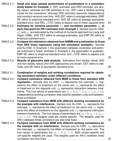
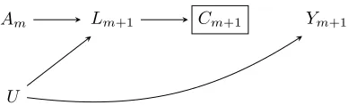
We next extend the method to time-varying treatments. Suppose that treatments and covariates

are measured repeatedly at timesm = 0, ..., K−1, and outcomes are measured only at the last time pointK. Figure 2.2 is a partial DAG that shows the effect of a joint treatment from two arbitrary time pointsm−1andmon the clustered outcomes at timem+ 1. The cluster-specific covariate

L†_m is omitted from the graph for simplicity. In this example,Lm = {Lm,1, Lm,2}is a time-varying confounder for the effect of Am = {Am,1, Am,2} on Y = {Y1, Y2}. Therefore, they need to be controlled for in analysis. Lm, however, also mediates the effect of earlier treatmentsAm−1onY,

which suggests that analysis should not control forLm. In addition,Lmis a collider on the pathway

fromAm−1toY. Controlling forLmwill thus induce bias in estimating the causal effect. For these

reasons, conventional regression methods will fail in the presence of time-varying confounding [14].

Lm,1

Lm,2

Am,1

Am,2

Ym+1,1

Ym+1,2

Am−1,1

Am−1,2

U

2.4.1. Structural nested mean models

In the SNMM below, the blip function vectorγ_m∗(.)models the effect of removing joint treatmentam at timemfrom both outcomes, after having removed the effect of all subsequent treatments.

E



 

Y¯am,0

1

Y¯am,0

2

¯

Lm= ¯lm,A¯m= ¯am



 −E



 

Y¯am−1,0

1

Y¯am−1,0

2

¯

Lm= ¯lm,A¯m= ¯am

  =    γ∗

m,1(¯am,¯lm;ψ)

γ_m,2∗ (¯am,¯lm;ψ)



 .

(2.10)

For repeatedly measured outcomes, (2.10) can be further generalized to

EYa¯m,0

m+1|L¯m= ¯lm,A¯m= ¯am

−EYa¯m−1,0

m+1 |L¯m= ¯lm,A¯m= ¯am

=γ∗

m(¯am,

¯_l

m;ψ), (2.11)

where γ∗

m is a vector with components γ ∗

m,k(¯am,¯lm;ψ) that models the effect of removing joint treatment at timem from both outcomes at timek, fork = m+ 1, ..., K. The sequential ignora-bility assumption is required to identify the contrast in (2.10) and (2.11). It is a generalization of

assumption A2 to sequential treatments as shown below:

Y¯am−1,0

m+1 ⊥Am|A¯m−1= ¯am−1,L¯m= ¯lm. A parameterized example for (2.10) is shown below:



 

γ∗_m,1(¯am,¯lm;ψ)

γ∗_m,2(¯am,¯lm;ψ)

  =   

ψm,1am,1+ψm,2am,2+ψm,3am,1am,2

ψm,10a_m,2+ψ_m,20a_m,1+ψ_m,30a_m,2a_m,1





. (2.12)

Theψparameters in (2.12) have similar interpretation as those in example (2.3), except that they contain subscript m to indicate the effect of joint treatment at time m is time-specific. A more parsimonious example is shown below:



 

γ∗_m,1(¯am,¯lm;ψ)

γ∗m,2(¯am,¯lm;ψ)

  =   

ψ1am,1+ψ2am,2+ψ3am,1am,2

ψ1am,2+ψ2am,1+ψ3am,2am,1





. (2.13)

Model (2.13) makes the symmetry assumption and also assumes the effect of treatments is the

interpreted as effect of treatment per unit time.

2.4.2. Estimation

Similar to the single time point case, we first construct a series of partially blipped down outcomes

Umfor each timem:

Um=

   Y1 Y2   −

K−1

X

l=m



 

γ_l,1∗ (¯al,¯ll;ψ)

γ_l,2∗ (¯al,¯ll;ψ)



 .

The partially blipped down outcomes mimic the potential outcomes Ya¯m−1,0 _{in the sense that}

E Um|L¯m,A¯m = E Y¯am−1,0|L¯m,A¯m. For repeatedly measured outcomes, Um is a vector with components

Um,k=

   Yk,1 Yk,2   −

k−1

X

l=m



 

γ_l,k,1∗ (¯al,¯ll;ψ)

γ_l,k,2∗ (¯al,¯ll;ψ)



 ,

fork=m+ 1, ..., K.

For time-varying treatments, we suggest using the following score:

Sψ= N

X

i=1 K−1

X

m=0

"

∂γ_m∗ L¯im,A¯im;ψ

∂ψT −E

(

∂γ_m∗ L¯im,A¯im;ψ

∂ψT ¯

Lim,A¯i,m−1

)#

·V arUim

¯

Lim,A¯i,m−1

−1

·

Uim−E Uim|L¯im,A¯i,m−1 . (2.14)

The efficient score in (2.6) is usually too complicated to be used for situations with time-varying

treatments. The estimator from the score in (2.14) is not optimal but is reasonably efficient and

dou-bly robust. It is straightforward to show that the estimator is consistent, if for each timem, either the model for treatment,E

∂γ_m∗(_L¯_m,A¯_m;ψ) ∂ψT

¯

Lm,A¯m−1

, or the model for outcome,E Um|L¯m,A¯m−1, is correctly specified. A simpler non-doubly robust estimating equation is

Sψ= N

X

i=1 K−1

X

m=0

"

∂γ_m∗ L¯im,A¯im;ψ

∂ψT −E

(

∂γ_m∗ L¯im,A¯im;ψ

∂ψT ¯

Lim,A¯i,m−1

)#

·Uim. (2.15)

For the parameterized example in (2.13), we have the following expression for ∂γ

∗

m(L¯m,A¯m;ψ)

∂ψT :

∂γ∗

m L¯m,A¯m;ψ

∂ψT =

     

Am,1 Am,2

Am,2 Am,1

Am,1Am,2 Am,2Am,1

      . Similarly, E

∂γ∗_m(L¯m,A¯m;ψ)

∂ψT

¯

Lm,A¯m−1

is based on a model for treatment. If treatment

proba-bilities are unknown, a multinomial logistic regression model can be used to estimate treatment

probability in each category of the combined treatment{Am,1, Am,2} received at timem. We can either fit a separate model for each time m, or fit a single model to pooled data from all person times. For the pooled treatment model, we may allow intercepts to be time-varying with the use of

a spline.

2.4.3. Closed form estimator

IfV ar Um|L¯m,A¯m−1

is given, and a linear working modelDmδ=dm L¯m,A¯m−1

δis assumed forE Um|L¯m,A¯m−1

, whereδ is the q−dimensional nuisance parameter in the outcome model anddmis aJ ×q matrix-valued function of

_¯

Lm,A¯m−1 , and the blip function is linear inψwith

γ∗

m L¯m,A¯m

=Rmψ=rm L¯m,A¯m

, whereψisp−dimensional andrmis aJ×pmatrix-valued function of_¯

Lm,A¯m , the estimator forψwill have the following closed form (based on Robins and Hern´an, 2009):

   ˆ ψ ˆ δ   =        N X i=1 K−1

X m=0    Cim Dim    T

·V arUim

¯

Lim,A¯i,m−1

−1

·

PK−1

l=mRil Dim

       −1 ·        N X i=1 K−1

X m=0    Cim Dim    T

·V arUim

¯

Lim,A¯i,m−1

−1

·Yi

       , (2.16)

whereCm=P K−1 l=m

Rl−E

Rl

L¯m,A¯m−1 . A simple working model forV ar Um|L¯m,A¯m−1

isσ2_I

section will examine the impact of such mis-specification on the efficiency of ψˆ. If one assumes a working model other than independence structure and constant variance, estimation will then

require iterative procedures similar to those in generalized estimating equations (GEEs). We can

start by assuming working modelσ2_I

J×Jto obtain an initial estimate forψ, and then iterate between estimating parameters inV arUm

¯

Lm,A¯m−1

and estimatingψ until convergence is achieved. We adapted the method of moments approach by Liang and Zeger (1986) in estimating variance

parameters [9]. An asymptotic variance estimator forψˆmay be derived using the sandwich method, with the exact form found in Appendix A.1.

2.5. Simulation study

2.5.1. Algorithm

The data generating process is based on the likelihood for SNMMs described in Robins, Rotnitzky

and Scharfstein (2000) [17]. Details about the likelihood can be found in Appendix A.2. A simulation

study is conducted based on the setting where treatments and covariates are measured repeatedly

at timesm= 0, ..., K−1, and outcomes are measured at the last time pointKonly. The number of time points is K = 5, and the cluster size isJ = 2. The total number of clusters is varied as

N = 100or 1000. The algorithm for generating data for one cluster is shown below. It includes two examples with different covariate effects in the conditional mean of outcomes. Variables with

subscriptm=−1assume value 0.

Form= 0, ..., K−1, we generated covariatesLmfrom a multivariate normal distribution:

      Lm,1 Lm,2

L†_m

     

|L¯m−1,A¯m−1∼N3

           

0.3Lm−1,1+ 0.2Am−1,1

0.3Lm−1,2+ 0.2Am−1,2

0.3Lm−1+ 0.1Am−1,1+ 0.1Am−1,2

      ,      

1 0.3 0.2 0.3 1 0.2 0.2 0.2 1

            .

We generated joint treatmentAm from a multinomial logistic regression model with probabilities

pm,00,pm,10,pm,01,pm,11:

   Am,1 Am,2   | ¯

where

pm,10=mlogit−1(0.5Lm,1−0.5L†m+ 0.2Am−1,1),

pm,01=mlogit−1(0.5Lm,2−0.5L†m+ 0.2Am−1,2),

pm,11=mlogit−1(0.5Lm,1+ 0.5Lm,2−L†1+ 0.2Am−1,1+ 0.2Am−1,2),

pm,00= 1−pm,01−pm,10−pm,11.

Last, observed outcomes YK were generated. We first generated the conditional mean of YK

under the sequential ignorability assumption:

E(YK|¯lK−1,¯aK−1) = K−1

X

m=0

γ_m∗(¯lm,¯am) + K−1

X

m=1

h

E(Yam−1,0

K |¯lm,a¯m−1)−E(Y am−1,0

K |¯lm−1,a¯m−1)

i

+E(Y_K0|l0).

For both simulation examples,

K−1

X

m=0

γ∗m(¯lm,¯am) = K−1

X

m=0



 

ψ1am,1+ψ2am,2+ψ3am,1am,2+ψ4am,1lm,1+ψ5am,1l†m

ψ1am,2+ψ2am,1+ψ3am,2am,1+ψ4am,2lm,2+ψ5am,2l†m



 ,

whereψ1= 2, ψ2= 0.5, ψ3= 0.2, ψ4= 0.5, ψ5=−0.2, and

E(Y0_K|l0) =



 

2l0,1−l†0

2l0,2−l†0



 .

The two examples differ in the association between covariates and the potential outcomes. In

Example 1, the association is linear:

K−1

X

m=1

h

E(Yam−1,0

K |¯lm,a¯m−1)−E(Y am−1,0

K |¯lm−1,a¯m−1)

i

=

K−1

X m=1        

lm,1−lm†

lm,2−lm†



 −E

     

lm,1−l†m

lm,2−l†m



 |

¯_{lm−1,¯am−1}

In Example 2, the association is quadratic:

K−1

X

m=1

h

E(Yam−1,0

K |¯lm,¯am−1)−E(Y am−1,0

K |¯lm−1,a¯m−1)

i

=

K−1

X m=1        

(lm,1−l†m) 2

(lm,2−l†m)2



 −E

     

(lm,1−lm† ) 2

(lm,2−lm† )2



 |

¯_{lm−1,a¯m−1}

        . (2.18)

YK was generated from its conditional mean plus a bivariate normal error term:

YK=E(YK|¯lK−1,¯aK−1) +,

where the error term also follows multivariate normal distribution:

|L¯K−1,A¯K−1∼N2



 0,



 

1 0.2 0.2 1

     . 2.5.2. Results

Two doubly robust (DR) estimators (2.14) and one without the doubly robust property (2.15) were

computed using the simulated data (Example 1). For both DR estimators, we assume a linear

work-ing model forE Um|L¯m,A¯m−1

. ForV arUm

¯

Lm,A¯m−1

, we either assume an exchangeable

working modelΣm=σ2m



 

1 ρm

ρm 1





for each timemand denote the estimator asDR1, or a

work-ing model with independence structure and constant varianceΣ = σ2

   1 0 0 1  

for all time points

and denote the estimator asDR2. TheDR2estimator has the closed form described in (2.16), but not theDR1estimator. The non-DR estimator is based on the score in (2.15).

To estimate treatment probabilities, a multinomial logistic regression model is fit to pooled data

from all time points. Simulation and estimation procedures were repeated for 1000 replicates. The

results are shown in Table 1. Averaged estimates (Ave EST), empirical standard errors (Emp SE),

and averaged asymptotic standard errors (Ave SE) are provided. The square root of mean squared

Coverage of all95%confidence intervals (CI) atN = 1000show the expected range of93%−96%. At N = 100, all 95% CIs show under-coverage, likely due to the small sample size. The DR1 estimator has the worst coverage probabilities at N = 100, but it is the most efficient among the three estimators. The relative √MSE of DR2 and non-DR estimators relative to DR1 estimator ranges from1.3−1.4 and 2.4−3.4 respectively. As seen in Table 2, for the DR1 estimator, the estimates of the variance parameterσ2

mand correlation parameterρmin the conditional variance of Umdecrease over time, since more of the variance is accounted for by the increased treatment and

covariate history in the conditioning. Therefore, a flexible working model forV arUm

¯

Lm,A¯m−1

used in DR1 estimator tends to improve efficiency.

We did a comparison between g-estimation of SNMMs and standard GEE regression, a

conven-tional method to deal with clustered outcomes. We considered two simulation examples with

differ-ent covariate effects as shown in (2.17) and (2.18). Both SNMM and GEE regression approaches

were applied to the simulated data. Predictors in restricted mean models for GEE include all factors

in the blip functions as well as all covariates used in generating the conditional mean of outcomes.

An exchangeable working model is assumed for the correlation structure. The conditional mean

models used in the GEE approach in the two examples are

Yj ∼ K−1

X

m=0

Amj+ K−1

X

m=0

Amj0+

K−1

X

m=0

AmjAmj0+

K−1

X

m=0

AmjLmj+ K−1

X

m=0

AmjLm+ K−1

X

m=0

Lmj+ K−1

X

m=0

Lm,

and

Yj∼ K−1

X

m=0

Amj+ K−1

X

m=0

Amj0

K−1

X

m=0

AmjAmj0+

K−1

X

m=0

AmjLmj+ K−1

X

m=0

AmjLm+

L0j+L0+ K−1

X

m=1

L2mj+ K−1

X

m=1

L2m+ K−1

X

m=1

Lmj·Lm

respectively. The models included correctly specified predictors, but did not properly control for

time-varying confounding. The coefficients corresponding to treatment and effect modification are

shown in Table 3. As expected, the DR1 estimators from SNMMs and g-estimation are unbiased,

whereas bias is induced in GEE estimators by controlling for covariates affected by earlier

treat-ments. In the first example, the GEE estimators are in fact more efficient than the DR1 estimators.

larger standard errors compared to the DR1 estimators, and all of them are biased.

2.6. Analysis of glaucoma data

The Ocular Hypertension Treatment Study (OHTS) is a multi-center randomized trial designed to

evaluate the safety and efficacy of topical ocular hypertensive medication in delaying or preventing

primary open-angle glaucoma in subjects with elevated intra-ocular pressure (IOP) [7]. In the first

part of the study, a total of 1636 subjects with an IOP between 24 mm and 32 mm in one eye and

between 21 mm and 32 mm in the other eye were randomized to either observation or treatment

with commercially available topical ocular hypertension medication. In the second part of the study,

both the observation arm and the treatment arm received medication. The subjects were followed

up every 6 months up to 7.5 years median time in the first part of the study and up to 13 years

median time in the second part.

We use data from 817 subjects in the treatment arm to illustrate our method. In the treatment

arm, the subjects received several classes of topical ocular hypertension medications, including

beta blockers, prostaglandin analogues, topical carbonic anhydrase inhibitors and alpha 2 agonists.

Sometimes more than one type of medication was prescribed for one eye. We are interested

in comparing the effectiveness of the two most common classes, beta blockers and prostaglandin

analogues in lowering IOP. The treatment is eye-specific drops, and the outcome is IOP in each eye.

Within the treatment arm, different medications were not randomized. At each visit, clinicians made

decisions about the type and dose of medication given to each subject, although dose information

is not available in the data provided. Treatment decisions at each time may be influenced by the

subject’s treatment and covariate history. Therefore, the treatment received by these subjects is

time-varying. The subject’s IOPs at each visit are affected by earlier treatment and IOPs, and in

turn affect later treatment and IOPs. Therefore, they are likely to be time-varying confounders.

We created a categorical treatment variable containing 3 categories: beta blocker only (BB), prostaglandin

analogue only (PROST) and beta blocker plus prostaglandin analogue (BB+PROST). Since almost

all subjects received medication only to one eye at baseline, we did not model baseline treatment

but still included relevant baseline covariates in our analysis. In the follow-up visits, once a subject

received no medication or medications other than a beta blocker and prostaglandin analogue in

subjects received a beta blocker at the first follow-up visit, treatment at the first follow-up visit was

also not modeled. In this study, most subjects did not receive different treatments in each eye.

Therefore, we decide not to model the effect of treatment on the opposite eye. For each eye, we

pooled all subject-visits and fit a pooled multinomial logistic model after performing model selection

based on AIC. The resulting treatment model was

mlogit Pr[Atj =a|A¯t−1,L¯t] =α0t+α1At−1,j+α2At−1,j0 +α₃IOP_t,j+α₄IOP_t,j0+α₅IOP_t−1,j+

α6At−1,j·IOPt−1,j +α7RACE +α8AGE +α9IOP0,j,

wherea= 1or2refers to ‘PROST’ or ‘BB+PROST’ versus the reference category ‘BB’. The signif-icant predictors include IOP in the current time in each eye, IOP in the previous time in the same

eye, treatment in the previous time in each eye, interaction between IOP and treatment in the

pre-vious time in the same eye, as well as baseline covariates race, age and baseline IOP in the same

eye. The time-varying intercept is modeled by a spline to allow more flexibility. The causal effect is

modeled with a blip function with two parameters

EYa¯m,0

k,j |L¯m= ¯lm,A¯m= ¯am

−EY¯am−1,0

k,j |L¯m= ¯lm,A¯m

=γ_m,k,j∗ (¯am,¯lm;ψ)

=ψ1I(am,j = 1) +ψ2I(am,j = 2),

whereψ1 represents the effect of ‘Prost’ versus ‘BB’, and ψ2 represents the effect of ‘BB+Prost’ versus ‘BB’. Negative values refer to lowering IOP more and therefore indicate that a treatment

is beneficial relative to ‘BB’. This model makes the symmetry assumption and also assumes the

effect of treatment at each time is the same on each of the later outcomes. Both non-doubly robust

(non-DR) and doubly robust (DR) estimators were computed forψ, and the results are shown in Table 2.4.

The DR estimators have smaller standard errors compared to the non-DR estimators. Results from

the DR approach show thatψˆ1= -0.15 with p-value= 0.22, suggesting the effect of ‘PROST’ is not significantly different from that of ‘BB’, andψˆ2= 0.19 with p-value= 0.047, suggesting the combined treatment ‘BB+PROST’ is significantly worse than ‘BB’ in lowering IOP. The fact thatψˆ2is positive is counterintuitive, since we would expect a combined treatment to work better than any of the single

model.

2.7. Discussion

In this work, we have extended SNMMs to settings with clustered observations and time-varying

confounding. We formulate models that are generalized to both cluster- and unit-level treatments,

with consideration of the effect of interference. We also derive semiparametric estimators of

param-eters in those models. Our simulation study demonstrated that the estimators are consistent and

achieve reasonable efficiency in contrast to those from the conventional GEE regression approach.

We have applied the method to compare the effectiveness of two commonly used topical ocular

hypertension medication in lowering IOP using data from the treatment arm of OHTS. In the

glau-coma study, two eyes of a given subject form a cluster. At each visit, different medications were

not randomized in the treatment arm. Therefore, it is a setting with clustered observations and

time-varying confounding. The effect of prostaglandin relative to beta-blocker is not shown to be

statistically significant. The fact that the effect of the combined treatment is shown to be worse

than that of the single treatments is counterintuitive. One likely explanation is residual

confound-ing in the analysis, since clinicians usually prescribe combined treatment if the sconfound-ingle ones do not

work. Some of the residual confounding may also be due to the lack of dose information, which

limits the capacity to fairly compare the three treatment categories. The analysis can potentially be

improved by adjusting for loss to follow-up and exclusion of patients on other medications through

inverse probability weighting (IPW). In this particular dataset, the treatment did not differ between

two eyes in most subjects. Simulation study suggests it is not suitable to model interference under

such situations because of the multicollinearity problem (results not shown). However, the method

introduced can potentially be used to model interference among units within the same cluster when

treatment assignments within the cluster are more variable.

We have demonstrated and implemented our method with continuous outcomes and an identity

link in SNMMs. Our method can potentially be generalized to discrete outcomes and other link

functions. For binary outcomes and the logit link, the causal parameter in SNMMs cannot be

estimated with G-estimation [13]. Vansteelandt and Goetghebeur (2003) proposed the generalized

structural mean model to overcome this limitation [28]. The two-stage model includes a structural

outcome in the treatment arm. They also proposed an estimator that is robust to misspecification of

the nuisance association model. The causal model in their approach can be extended to clustered

observations in a similar way described in our method. Extensions of the association model to

T ab le 2.1: Small and lar g e sample perf ormance of g-estimator s in a sim ulation stud y based on Example 1 . DR1 estimator and DR2 estimator are doub ly rob ust, whereas no n-DR estimator is not. DR1 uses a fle xib le w or king model for the co v ar iance , whereas DR2 estimator assumes independence and constant v ar iance o v er time . A VE EST ref ers to a v er age estimates , EMP SE ref ers to empir ical st andard error , A VE SE ref ers to a v er age asymptotic standard error , and REL √ MSE ref ers to square root of mean squared error . DR1 Estimator DR2 Estimator non-DR estimator N P ar am T rue A v e EST Emp SE A v e SE 95% _CO V √ MSE A v e EST Emp SE A v e SE 95% _CO V

REL _√ MSE

A v e EST Emp SE A v e SE 95% _CO V

REL _√ MSE

Table 2.2: Estimates for variance parameterσ2

m and correlation parameterρmat each time

point for DR1 estimator fromExample 1. Sample size N=1000.σ2

mandρmare estimated by the method of moments approach by Liang and Zeger (1986). AVE EST refers to average estimates, and EMP SE refers to empirical standard error.

ˆ

σ2m ρˆm Time (m) Ave

EST Emp

SE

Ave EST

Emp SE 0 7.76 0.38 0.51 0.03 1 6.06 0.29 0.50 0.03 2 4.37 0.19 0.47 0.03 3 2.69 0.11 0.42 0.03 4 1.03 0.03 0.19 0.03

Table 2.3: Compare the estimators obtained from SNMM and g-estimation to those from GEE linear regression using two simulation examples. Sample size N=1000. InExample 1, the association between covariates and potential outcomes is linear, whereas inExample 2, the association is quadratic. EMP SE refers to empirical standard error, and√MSE refers to square root of mean squared error.

DR1 estimator GEE estimator

Example Param True Bias Emp

SE Bias Emp

SE

REL

√

MSE

1

ψ1 2.0 -0.00 0.05 -0.08 0.03 1.69

ψ2 0.5 -0.00 0.05 0.08 0.03 1.71

ψ3 0.2 0.00 0.07 0.00 0.04 0.61

ψ4 0.5 0.00 0.03 0.00 0.02 0.56

ψ5 -0.2 -0.00 0.03 0.00 0.02 0.62

2

ψ1 2.0 -0.00 0.06 -0.17 0.10 3.07

ψ2 0.5 -0.00 0.07 -0.02 0.09 1.46

ψ3 0.2 0.00 0.09 0.07 0.13 1.58

ψ4 0.5 0.00 0.04 0.14 0.06 3.56

ψ5 -0.2 0.00 0.04 -0.31 0.06 7.25

Table 2.4: Results of glaucoma data analysis. Estimators from doubly robust (DR) and non-doubly robust (non-DR) approaches are shown. EST refers to estimate, and SE refers to asymptotic standard error.

Non-DR estimator DR estimator EST SE P-Value EST SE P-Value

ψ1 -0.27 0.34 0.21 -0.15 0.20 0.22

CHAPTER 3

M

TIME

-

3.1. Introduction

Marginal structural models (MSMs) are a class of causal models useful for estimating the effect

of time-varying treatments in the presence of time-varying confounding [15]. An MSM is structural

because it is a model for counterfactual outcomes, defined as outcomes that would be observed

were the subject to receive a certain treatment [20]. It is marginal because it describes the effect of

pre-specified treatment regimes on the marginal distribution of their corresponding counterfactual

outcomes. The parameters of an MSM can be consistently estimated by the use of inverse

proba-bility weights (IPW) that create a pseudo-population in which the distribution of confounders is the

same in the treated and the untreated. Therefore, the pseudo-population is free from confounding.

Structural nested models (SNMs) are another major class of causal models that can be used to

deal with time-varying confounding. MSMs are more widely used than SNMs, partly because the

models are easier to understand and can be implemented with standard software. However, both

methods have their respective advantages. Brumback et al. (2014) and He and Marshall (2014)

introduced SNMs for clustered observations [1] [3]. This paper focuses on formulating MSMs for

clustered observations.

A motivating example of eye disease treatment was introduced by Heitjan and Sharma (1997), He

and Joffe (2014), where two eyes of a given subject form a cluster [4] [3]. Eye-specific outcomes

from a given subject tend to be correlated because they share subject-specific characteristics.

Rubin (1986) calls a situation where “the observation on one unit is unaffected by the particular

treatment assignment to the other units the “stable unit-treatment value assumption (SUTVA)” [19].

If we consider each eye as a separate unit for treatment, the SUTVA assumption may be violated.

Under eye-specific treatment, treatment received by one eye may affect the outcome in the other

eye of the same subject. If the treatments are binary, each eye will have not only two but four

potential outcomes, depending on the treatment received by both eyes. In the ophthalmology study,