436 | International Journal of Computer Systems, ISSN-(2394-1065), Vol. 02, Issue 10, October, 2015
Available at http://www.ijcsonline.com/
Clustering Analysis Using Hierarchy Grouping
Arthur Smirnov
1, 2, Valery V. Sharlay
3, Valery V. Pelenko
4, Aleksandr V. Baranenko
4, Valdur Aret
41Department of Computer Science, University of Illinois at Chicago, Chicago IL, USA 2Machine Intelligence Research Labs (MIR Labs), WA, US
3
Institute of Information Systems and Data Protection, St. Petersburg State University of Aerospace Instrumentation, St. Petersburg, Russia
4Institute of Refregiration and Biotechnologies, St. Petersburg, Russia
Abstract
We consider various techniques of grouping with different parameters.
Keywords: Dendrogram, clustering, analysis, Euclidian Set.
I. INTRODUCTION
In this paper we consider different types of grouping using and testing various techniques. We explain in details and apply evident grouping, hierarchical grouping, and also agglomerative hierarchical grouping. We provide various graphs with samples that are applicable to a certain type of grouping.
II. EVIDENTGROUPING
Evident grouping is a classification of the object of the study which is defined by a set of observations is assigning this object to one of the mutually exclusive classes K = {K1, K2, …, KM}. Classes are defined standards
H = {H1, H2, … , Hm} in the dimension of features Y =
φ(X). The standards are constructed during the process of training. Training without a trainer requires a priori information and, of course, a higher value of the error [1].
Alternative way to classifying consists of grouping features, namely speaking selecting clusters out. This way actually groups points of features by having common properties. Grouping (clustering analysis) is a non-parametric procedure which does not require describing features by any kind of distribution.
Let’s have a certain set which has a set of points Y; these points have to be grouped by a similarity of features. The most common criteria used in such cases are distance between points. It is obvious that the distance among points within one cluster will be less than the distance between any two clusters [2]. This distance can be calculated in different ways. In the n-dimensional Euclidean space distance between points yi, yj will be as following:
2
21 1
...
ij i j in jn
r
y
y
y
y
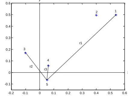
Graph 1 and table 1 demonstrate a set of five points (2-dimensional Euclidian space).
-0.2 -0.1 0 0.1 0.2 0.3 0.4 0.5 0.6 -0.1
0 0.1 0.2 0.3 0.4 0.5 0.6
1 2
5 4 3
x y
r1
r2 r3
Graph 1. Set of five points in 2D Euclidean Space Table 1. Coordinates of five points listed above.
№ 1 2 3 4 5
x 0.5380 0.3991 -0.1011 0.0614 0.0508 y 0.4980 0.4952 0.1692 0.0591
-0.0644
0
0.1390
0.7187
0.6479
0.7441
0.1390
0
0.5970
0.5515
0.6591
0.7187
0.5970
0
0.1963 0.2786
0.6479
0.5515
0.1963
0
0.1239
0.7441
0.6591 0.2786
0.1239
0
R
Method of grouping: two points belong to the same cluster if the distance between these two points is less than critical distance r0. Maximum distance r1 = 0.7441 between points 1 and t; if we set r0 > r1, then all five points will belong to the same cluster, and there will only be one cluster. Minimum distance r3 = 0.1239 between points 4 and 5, and if we set r0 > r3, then none of the points will be combined under same cluster; in this case we will have five clusters consisting of only one point each. If we set r0 ~ r2 = 0.2786, the following distances will be less than r0: r12, r34, r35, r45, but the distance between points 1, 3, 4 and 5 and also between points 2, 3, 4, and 5 will be more than r0, thus we have two visually obvious clusters: K1 = {θ1, θ2} and K3 = {θ3, θ4, θ5}.
In practice points may have different criteria to separate from, such as color, size, object shape etc. This may be compared to uniform and non-uniform sampling difference [3]. It is always important to have a criteria defined which will be used for separating points. There could be multiple criteria initially visually chosen, but only one of these criteria will be an optimized one.
III. HIERARCHIRALGROUPING
Let’s have N sets of data which have to be grouped into n subsets (clusters Ki, i = 1,…,n) with unknown sizes mi,
i i
m
N
If the criteria of grouping this data has been set, then we can find a maximizing value of the criteria by a simple sorting. But due to a fact of not knowing a size of clusters (value of m i in the range of 1 to N) the number of these maximizing values can be very big even for a modern machine:
!
N
K
n
N
n
That said above, in order to split the set with N = 50 into n=10 subsets, we have to sort out
43
3.10
KN
options.
Another way of to select some data and “moving” data from one cluster to another if it improves the criteria (iterative optimization). Various initial approximations can lead to various solutions, but computational complexity of the procedure is acceptable.
Obvious way to partition N points is splitting these points into N groups by having only one point in group. Then we can partition into N-1 groups, then into N-2 and so on. The process of partitioning is on the k-th level if n = N – k + 1: the first level represents N groups, N-th level represents one group. Hierarchy grouping is such grouping when the same two points grouped on the k-th level stay grouped on higher levels.
Graphically speaking this hierarchy looks like a tree which has the same structure as and is called a dendrogram [4]. Let’s consider another example.
Table 2. Set of points. N = 7 points
№ 1 2 3 4
X -0.1364
0.1 139
1.0 688
0.0 593
№ 5 6 7
X
-0.0956 -0.8323
0.2 944
CONCLUSION
Graph 2. Set of points. N = 7 points.
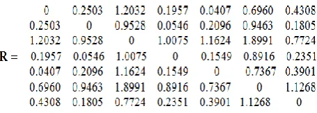
Criteria of classification – minimum Euclid distance. The matrix of distances is shown below:
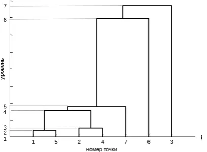
On the first level of classification N=7 groups stand out by one isolated point in each group. Minimum distance r2 =
0.0407 between two points x1 and x5 – at the second level
of grouping (pic. 3) Next minimum distance is r3 = 0.0546
-1 -0.5 0 0.5 1 1.5
1 4
6 5 2 7 3
between points x2 and x4, these points are grouped on the
third level. The next minimum distance is r4 = 0.1549
between points x4 and x5, which belong to already existing
groupings, that is why are combined on the fourth level. By the same criteria are defined the distances for r5 = r27, r6 =
r56, r7 = r36 are grouped on the fifth, sixth and seventh
levels.
1 5 2 4 7 6 3 номер точки
ур
ов
ен
ь
i 1
2 3 45 6 7
Graph 3. Dendrogram
Clusters from sets of groups of dendrograms can vary by various features, for example, by their a priori by the detected number. If in this example the grouping needs three clusters, then result (pic. 2 and pic. 3): K1 = {x6}, K2
= {x3}, K3 = {x1, x2, x4, x5, x7}. If groupings needs two
clusters, then K1 = {x1, x2, x4, x5, x6, x7}, K2 = {x3}.
IV. AGGLOMERATIVEHIERARCHIRAL
GROUPING
Hierarchical procedure starting from separate points is called agglomerative. A number of combining groups must be defined otherwise this procedure will combine all points into one group[5]. Algorithm is as following:
There is a certain rule θ which is applicable to combining groups Σi, Σj. In example 3 on the k-th level the
following rule was applied: Θk=min{R
e
ij}, I,j = 1,…, N-k+1- Euclid distances of
Reij were calculated between all pairs of groups N-k+1 the
pair with the smallest distance was chosen. In the rule listed above other than Euclid distance, other parameters can be used instead. In order to measure the distance between groups are calculated as following:
,
min
i,
jsng
i
j
r
x
y
x
y
,
,
max
i, jcomp i j
r
x yx y
,
1
,
i j
avg i j
i j
r
n n
x y
x
y
,
,
mean i j i j
r
m
m
, Where ||x-y|| = rxy – distance between points x and y.It is important to note that various artificial intelligence techniques can be applied at the stage of agglomerative hierarchical grouping due to a complexity of this method.
V. NEARESTANDFURTHESTNEIGHBOR
ALGORITHM
These algorithms are more revealing from the point of view of grouping [7]. Let’s consider an example of 2D Euclidian coordinates X, m = 5 points create a distance Y. We use a function Y = pdist (X), where i and j are numbers of points.
Table 3. Distances of Y function
k 1 2 3 4
i, j 1-2 1-3 1-4 1-5
Yk 0.5839 0.1484 0.3140 0.6454
K 5 6 7 8
i, j 2-3 2-4 2-5 3-4
Yk 0.6614 0.8168 0.2020 0.1726
k 9 10
i, j 3-5 4-5
Yk 0.755
2
0.923 5
Now we will consider the nearest neighbor algorithm: upper triangle matrix is a block of matrix of distances r.
0
0.5839
0.1484
0.3140
0.6454
0
0.6614
0.8168
0.2020
0
0.1726
0.7552
0
0.9235
0
On the second level based on the minimal distance r13 =
Z = 1.0000 3.0000 0.1484 % Υ2
6.000 4.000 0.1726 % Υ3
0 0 0 0 0 0
We now exclude r34 and r14 (because points x1, x3 and
x4 are now combined) into a triangle matrix on the fourth
level.
0
0.5839
0.3140
0.6454
0
0.6614
0.8168
0.2020
0
0.1726
0.7552
0
0.9235
0
Minimal distance r25 = 0.2020. None of the points x2 or
x5 belong to the group Υ3, therefore these points are not
neighbors and construct a separate group Υ4 = {x2, x5} and
we get the following matrix (% means a cluster on the second lever, its number is 8):
Z = 1.0000 3.0000 0.1484 % Υ2
6.0000 4.0000 0.1726 % Υ3
2.0000 5.0000 0.2020 % Υ4
0 0 0
r25 is being excluded. On the last fifth level in the
triangle matrix we get the following:
0 0.5839 0.6454
0 0.6614 0.8168
0 0.7552
0 0.9235
0
Minimal distance r12 = 0.5839. The nearest neighbors
will be groups Υ3, Υ4 and constructed the following matrix
(matrix (% means a cluster on the second lever, its number is 5):
Z = 1.0000 3.0000 0.1484 % Υ2
6.000 4.0000 0.1726 % Υ3
2.000 5.000 0.2020 % Υ4
7.000 8.000 0.5839 % Υ5
Graph 4. Dendrogramm. Nearest Neighbor Algorithm
Now we will consider the furthest neighbor algorithm: the main difference is that such elements or clusters of previous levels, which have a maximal distance inside of Kj (between furthest neighbors) turns out to be minimal,
are included into a new Kj [8].
We apply a new function linkage (Y’, co’) to the same data listed in table 3. Clusters of first and second level are the same ones as before, second level group Υ2 = {x1, x3}
combines the nearest points (these points are also the furthest neighbors). Triangle matrix of the third level looks as following:
0
0.5839
0.3140
0.6454
0
0.6614
0.8168
0.2020
0
0.1726
0.7552
0
0.9235
0
Distance r25= 0.2020 turns out to be the minimal
distance for all combinations of uniting pairs of points with the group Υ2. In the group Υ2 = {x2, x5} points x2, x5 – are
the furthest neighbors.
% - cluster of the third level, its number is 7: Z = 1.0000 3.0000 0.1484 % Υ2
2.0000 5.0000 0.2020 % Υ3
0 0 0 0 0 0
Analysis of triangle matrix of the fourth level gives us the following results:
0
0.5839
0.3140
0.6454
0
0.6614
0.8168
0
0.1726
0.7552
0
0.9235
0
It shows that the remaining point x4 is the furthest
neighbor of group Υ2, In the group Υ4 = {Υ2, x4} the furthest
% - cluster of the third level, its number is 8: Z = 1.0000 3.0000 0.1484 % Υ2
2.0000 5.0000 0.2020 % Υ3
6.0000 4.0000 0.3140 % Υ4
0 0 0
Finally groups Υ3 and Υ4 are combined. Graph 4 and
Graph 5 (the following one) don’t look have a lot of difference.
Graph 4. Dendrogramm. Furthest Neighbor Algorithm.
VI. CONCLUSION
We have shown how type of grouping can directly and indirectly influence the results of clustering. The value of the error also depends on type of grouping. We explained how different rules should be, if applicable, applied to a grouping. The Nearest Neighbor Algorithm has an advantage at chain constructing when the groups of points are extended. But the Furthest Neighbor Algorithm has very efficient when the groups of points are compact and the groups are relatively the same (sizes).
REFERENCES
[1] Scott, A.J., and M. Knott. “A cluster analysis method for grouping means in the analysis of variance.” iBiometrics (1974): 507-512 [2] Milone, Diego H., et all. “Improving clustering with metabolic
pathway data. “BMC Bioinformatics 15.1 (2014): 101.
[3] Smirnov, Arthur, A. Abraham, and S. Vorobiev. "The potential effectiveness of the detection of pulsed signals in the non-uniform sampling." IEEE.-2013 5: 137-139.
[4] Phipps, J. B. "Dendrogram topology." Systematic Biology 20.3 (1971): 306-308.K. Elissa, “Title of paper if known,” unpublished. [5] Smirnov, Arthur. Artificial intelligence: Concepts and Applicable
Uses. LAP LAMBERT Academic Publishing, 2013.
[6] Selinger, Andrea, and Randal C. Nelson. "A perceptual grouping hierarchy for appearance-based 3d object recognition." Computer Vision and Image Understanding 76.1 (1999): 83-92.
[7] Taneja, Shweta, et al. "An Enhanced K-Nearest Neighbor Algorithm Using Information Gain and Clustering." Advanced Computing & Communication Technologies (ACCT), 2014 Fourth International Conference on. IEEE, 2014.