Improving Transient Stability of Multi-Machine AC/DC Systems via Energy-Function Method

e-ISSN: 2278-067X, p-ISSN: 2278-800X, www.ijerd.com

Volume 10, Issue 8 (August 2014), PP.35-50

Improving Transient Stability of Multi-Machine AC/DC Systems

via Energy-Function Method

1

M Shobha,

K.Durga Rao,

Tegala.Srinivasa Rao

,

1_{P.G Student Scholar,} 2_{Assistant Professor,} 3 _{Associate Professor} 1,2,3_{Department of Electrical & Electronics Engineering}

1,2,3_{Avanti Institute of Engineering & Technology, Makavaripalem(P),Vishakhapatnam}

(Dt), Andhra Pradesh, India.

Abstract:- In this paper, the direct method of stability analysis using energy functions is applied for multi-machine AC/DC power systems. The system loads including the terminal characteristics of the DC link are represented as constant current type loads, and their effects on the generators at the internal nodes are obtained as additional bus power injections using the method of distribution factors, thus avoiding transfer conductance terms. Using the centre of angle formulation, a modified form of the energy-function method is used for the swing equations and the DC link dynamical equations to compute the critical clearing time for a given fault. Numerical results of critical clearing time for a single and multi-machine system using the energy-function method agree well with the step-by-step method.

Index Terms:- Direct Current Link, Energy Function, External Control Signal.

I.

INTRODUCTION

Direct methods for analyzing power system stability have been applied successfully so far for pure AC systems. The literature on this topic is vast and was summarized in a survey paper by Fouad in 1975. Since 1975, there has been a significant advance in this research area, which has helped to remove the conservative nature of the results associated with this method in the past. Hence, the possibility of using this technique for transient security assessment is now quite good.

Since DC links are now being introduced for economic and other reasons, there is a need to extend the direct method of stability analysis to systems containing such links. It is well known that the quick response of the DC link, as opposed to an AC line combined with an effective control scheme, can enhance transient stability. The degree of transient stability for given fault is either the critical clearing time or the critical energy. The application of the direct method of stability analysis to AC/DC systems is not a routine extension of the method as applied to AC systems. Instead, it requires a different approach based on treating the post fault DC link dynamics as a parameter variation in the swing equations. A simplified first-order model of the DC link controller is proposed, which augments the usual swing equation for the machine. For the multi-machine case, the method using distribution factors is proposed to reflect (at the internal nodes) the terminal characteristics of the DC link and the system loads as additional power injections. This eliminates automatically the problem of transfer conductances in the swing equations. The computational algorithm and results for a multi-machine system are presented.

II.

SYSTEM

DESCRIPTION

A. Multi-Machine AC/DC System

𝐾𝑎 = 1.0 pu/rad per sec, 𝑇𝑑𝑐 = 0.1 sec, 𝑃𝑟𝑒𝑓 = 0.0

for both prefault and postfault conditions. 𝑃𝑟𝑒𝑓 is assumed to be zero for the sake of convenience. In general,

𝑃𝑟𝑒𝑓 will have different values in the prefault and postfault states, as in the single-machine case; and AC/DC load flow calculations have to be performed for each condition. Maximum 𝑃𝑑𝑐 = −2.0 pu; minimum; 𝑃𝑑𝑐 =

−2.0 pu; 𝑞𝑟 = 0.5. The external control signal (ECS) is chosen to be the difference between the rotor speeds of the generator nearest to the rectifier and inverter terminals, i.e., 𝑢 = 𝜔3− 𝜔1.

The extension of the method to multi-machine AC/DC systems involves a new method of handling system loads and DC link characteristics in the swing equations, as well as the use of the potential energy boundary surface method [3, 13] for computing 𝑉𝑐𝑟.

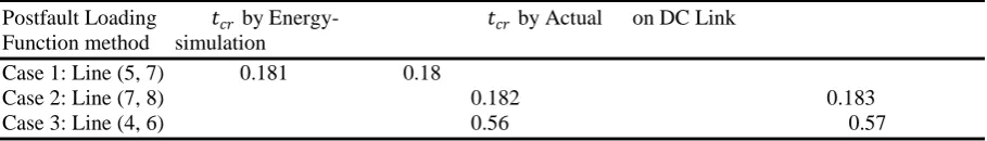
TABLE I Comparison of 𝒕𝒄𝒓 by Energy-Function method and Actual simulation Postfault Loading 𝑡𝑐𝑟 by Energy- 𝑡𝑐𝑟 by Actual on DC Link Function method simulation

Case 1: Line (5, 7) 0.181 0.18

Case 2: Line (7, 8) 0.182 0.183

Case 3: Line (4, 6) 0.56 0.57

B. Representation of the Effect of Loads

It is well known that the transfer conductances present in the internal bus description using the classical model pose a problem in constructing a valid V-function, as well as in computing 𝑡𝑐𝑟. These transfer conductances are mostly due to the system loads being converted to constant impedances and subsequent elimination of the load buses. In the method proposed here, which also applies to the DC link element, the effect of loads is reflected at the internal buses in the form of additional bus power injections.

Consider a power system network consisting of n buses and m generators. The bus admittance matrix 𝑌𝐿𝐿 for the transmission network alone, excluding the loads and DC link, is formulated and is thus augmented with the network elements corresponding to direct axis reactances of the m machines. The resulting augmented matrix 𝑌𝐵𝑢𝑠 has (n + m) buses altogether, and is represented as

(1)

where 𝑌𝐺𝐺, 𝑌𝐺𝐿, 𝑌𝐿𝐺, and 𝑌𝐿𝐿 are submatrices of dimensions (m x m), (m x n), (n x m), and (n x n) respectively. The overall network representation is

where

𝐼𝐺𝑡 = 𝐼𝐺1, 𝐼𝐺2, … 𝐼𝐺𝑚 , 𝐼𝐿𝑡 = 𝐼𝐿1, 𝐼𝐿2… . 𝐼𝐿𝑛

𝐼𝐺 and 𝐼𝐿 are the current injections at the internal nodes of the generators and the transmission network nodes, respectively; 𝐸𝐺 and 𝑉𝐿 are the associated voltages. 𝑌𝐵𝑈𝑆 is computed for the faulted and postfault conditions by properly taking the corresponding network changes into account. The method of distribution factors are suggested in [15] is now used for reflecting loads at the internal buses. Eliminating 𝑉𝐿 from Eq. (3.2), we get

𝑉𝐿= 𝑌𝐿𝐿−1𝐼𝐿− 𝑌𝐿𝐿−1𝑌𝐿𝐺𝐸𝐺 (3) and

𝐼𝐺= 𝑌′ 𝐸𝐺+ 𝐷𝐿 𝐼𝐿 (4) where

𝑌′ = 𝑌𝐺𝐺− 𝑌𝐺𝐿𝑌𝐿𝐿−1𝑌𝐿𝐺

and the distribution factor matrix for loads is given by

𝐷𝐿 = 𝑌𝐺𝐿𝑌𝐿𝐿−1 (5) Also, we have

(6) where 𝑃𝐿𝑗 and 𝑄𝐿𝑗 are the active and reactive power components of load at the jth bus. The additional bus power injections at the internal bus of the kth generator (k = 1, 2….m) due to the load at jth bus (j = 1, 2 ….n) is obtained as follows

(7)

Where 𝑑𝑘𝑗 is the appropriate (k, j) element of 𝐷𝐿 . The following assumption is made regarding the load

characteristics: the complex ratio of voltages 𝐸𝑘 _𝑉 𝐿𝑗

is assumed to be constant, corresponding to the prefault values. This is a deviation from the conventional type of representation of loads as constant impedances. Since only active power is of interest in the swing equation, we get

∆𝑃𝑘𝐿𝑗 = 𝑎𝑘𝐿𝑗𝑃𝐿𝑗 − 𝑏𝑘𝐿𝑗𝑄𝐿𝑗 (8)

The effect of all the loads at the internal bus of the kth generator is then obtained as

(9) C. Representation of the Effect of DC Link

(10)

where

𝐼𝐷𝑡 = 𝐼𝑟, 𝐼𝑖 , 𝑉𝐷𝑡= 𝑉𝑟, 𝑉𝑖

Subscripts r and I refer to the rectifier and inverter sides, respectively, and 𝑌𝐺𝐺′ , 𝑌𝐺𝐷, 𝑌𝐷𝐺, 𝑌𝐷𝐷 are submatrices of

dimensions (m x m), (m x 2), (2 x m), and (2 x 2), respectively. From Eq. (10), we get

𝑉𝐷= 𝑌𝐷𝐷−1𝐼𝐷− 𝑌𝐷𝐷−1𝑌𝐷𝐺𝐸𝐺 (11) and

𝐼𝐺= 𝑌′′ 𝐸𝐺+ 𝐷𝐷 𝐼𝐷 where

𝑌′′ = 𝑌𝐺𝐺′ − 𝑌𝐺𝐷𝑌𝐷𝐷−1𝑌𝐷𝐺

and the distribution factor matrix for the DC link is given by

𝐷𝐷 = 𝑌𝐺𝐷𝑌𝐷𝐷−1 (12)

Now, we represent the effect of the DC link currents 𝐼𝐷 as additional bus power injections at the internal buses of the generators. We have

and

(13) where

𝑃𝑟 = −𝑃𝑖 = 𝑃𝑑𝑐 and

𝑄𝑟 = 𝑄𝑖 = 𝑄𝑑𝑐

It is assumed here that the DC link is lossless and the power factors at the rectifier and inverter stations are equal. 𝑃𝑑𝑐 and 𝑄𝑑𝑐 are the active and reactive power components of the DC link that depend upon the DC link controller dynamics. The effect of the rectifier and inverter ends of the DC link as additional bus power

injections at the internal bus of the generator is given by

(14)

(15) where 𝑑𝑘𝑟 and 𝑑𝑘𝑖 are the appropriate (k, 1) and (k, 2) elements of the matrix 𝐷𝐷 .

From Eqs. (14) and (15), we get

and

∆𝑃𝑘𝑖 = −𝑎𝑘𝑖𝑃𝑑𝑐− 𝑏𝑘𝑖𝑄𝑑𝑐

As in the case of the load model representation, here also the ratios 𝐸𝑘 _𝑉 𝑟

and 𝐸𝑘 _𝑉 𝑖

are assumed to be

constant, corresponding to their prefault values. Since a simple structure is assumed for the DC link controller, the output of which is Pdc, let Qdc = qr Pdc, where qr is a constant.

From Eq. (16), we get the total bus power injections at the kth generator due to the DC link as ∆𝑃𝑘𝐷 = ∆𝑃𝑘𝑟+ ∆𝑃𝑘𝑖 = 𝑎𝑘𝑟 − 𝑎𝑘𝑖 − 𝑞𝑟(𝑏𝑘𝑟+ 𝑏𝑘𝑖)}𝑃𝑑𝑐

= 𝑐𝑘𝐷𝑃𝑑𝑐 𝑘 = 1,2 … . 𝑚 (17)

Where ckD is the expression in brackets in Eq. (17).

The parameters, (k = 1, 2…m, j = 1, 2…n),

which reflect the effect of the loads and the DC link, are thus computed for both the faulted and postfault condition. By kron reduction technique, the bus admittance matrix 𝑌𝐵𝑈𝑆 is reduced to the internal nodes of the generators for these two conditions.

C. Inclusion of DC link Dynamics

A structure similar to that described earlier is assumed for the DC link controller whose equations in terms of

𝑃𝑑𝑐 are 𝑃𝑑𝑐 = − 1 _𝑇

𝑑𝑐 𝑃𝑑𝑐 +

𝑃𝑟𝑒𝑓

𝑇𝑑𝑐+

𝐾𝑎

𝑇𝑑𝑐 𝑢 (18)

Where u is the external control signal (ECS) obtained from the AC system quantities, such as the difference in rotor speed of adjacent generators. The DC link dynamics are incorporated into the transient stability analysis in manner similar to the approach described earlier. Also, 𝑃𝑑𝑐 is constrained to vary with in the specified practical limits. While the faulted system equations are integrated, Eq. (18) also is solved for 𝑃𝑑𝑐. At the end each time step, the additional bus power injections at the internal buses of the generators are calculated using Eq. (17). The effect of DC link is thus represented as the term that modifies the power input of the generator.

III. System Equations

Under the usual assumptions [1] for the classical model, and following notation in [2], the system equations in the centre-of-angle reference frame are

𝑀𝑘𝜔 = 𝑃𝑘 𝑘− 𝑃𝑒𝑘 − 𝑀𝑘

𝑀_𝑇𝑃𝐶𝑂𝐴 𝜃𝑘 = 𝜔𝑘 k = 1, 2….m

(19) where

𝑃𝑘= 𝑃𝑚𝑘 − ∆𝑃𝑘𝐿− ∆𝑃𝑘𝐷− 𝐸𝑘 2𝐺𝑘𝑘 𝑃𝑒𝑘 = 𝑚𝑗 =1 𝐶𝑘𝑗sin 𝜃𝑗𝑘+ 𝐷𝑘𝑗cos 𝜃𝑘𝑗

≠𝑘

𝐶𝑘𝑗 = 𝐸𝑘 𝐸𝑗 𝐵𝑘𝑗 ; 𝐷𝑘𝑗 = 𝐸𝑘 𝐸𝑗 𝐺𝑘𝑗 and

𝜃𝑘= 𝛿𝑘− 𝛿𝑜

Where 𝛿𝑜 is the centre of angle defined by

𝑀𝑇𝛿𝑜= 𝑘=1𝑚 𝑀𝑘𝛿𝑘 , 𝑀𝑇= 𝑚𝑘=1𝑀 𝑘

𝑀𝑇𝜔𝑜 = 𝑚𝑘=1𝑃𝑘− 2 𝑚 −1𝑘=1 𝑚𝑗 =𝑘+1𝐷𝑘𝑗cos 𝜃𝑘𝑗

≜ 𝑃𝐶𝑂𝐴 (20)

In our formulation, since the system loads are not converted into constant impedances, the transfer conductance terms are only due to the transmission lines and hence can be neglected, i.e., 𝐷𝑘𝑗 = 0. If the angle is constant, i.e., 𝑃_𝑘 = 0, then 𝑃𝐶𝑂𝐴 = 0 [13]. The postfault SEP is obtained by solving the set of nonlinear equations 𝑃𝑘= 𝑃𝑒𝑘 k = 1, 2…..m-1 (21) Solution of these power flow equations is discussed extensively in the literature [13, 14].

A. Transient Energy Function

The transient energy function used is that given in [2], assuming the damping to be zero

= kinetic energy (KE) + rotor potential energy (PE) + magnetic potential energy (PE)

= 𝑉𝑘 𝜔 + 𝑉𝑝 𝜃 (22) where

𝑉𝑝 𝜃 = rotor PE + magnetic PE

B. Computing𝑉𝑐𝑟

Following [3], 𝑉𝑐𝑟 is computed as the value of 𝑉𝑝 along the sustained fault trajectory at the instant 𝑉𝑝 = 0. This happens to be a point on the so-called potential energy boundary surface (PEBS) [13]. An assumption is made that the PEBS crossing of the faulted trajectory is a good approximation to the value of 𝑉𝑐𝑟, which is the value of V(x) at the controlling UEP [3, 13].

C. Computational Algorithm

The algorithm for calculating the critical clearing time based on the proposed method is as follows: 1. Load flow calculation is performed for the prefault AC/DC system.

2. For the faulted and postfault states, the following computations are performed by augmenting the passive network with generator reactance.

a. The overall 𝑌𝐵𝑈𝑆 is computed excluding the loads and the DC link.

b. The distribution factors due to the system loads and DC link characteristics are computed as explained earlier.

c. The 𝑌𝐵𝑈𝑆 above is reduced to the internal buses of generators by eliminating all other buses. In doing so, the transmission line resistance is neglected.

3. The postfault SEP is computed by solving the nonlinear Eq. (21).

4. The faulted Eqs. (18) & (19) are numerically integrated to obtain values of 𝜃, 𝜔 , 𝑃𝑑𝑐 at 𝑡 = ∆𝑡. At the end of the integration interval, the following computations are done.

a. 𝑃𝑑𝑐 obtained from Eq. (18) is used in updating the bus power injections for both faulted and postfault states.

b. 𝑃𝑘 is accordingly modified in Eq. (19), and the new postfault SEP 𝜃𝑠 is computed by solving Eq. (21).

c. Using the updated values of 𝜃𝑠_{, the V-function in (22), as well as 𝑉}

d. The integration is now continued for the faulted Eqs. (18) and (19) and steps (a) - (c) are

repeated at 𝑡 = 2∆𝑡. For the sustained fault trajectory, this is continued until 𝑉𝑝 changes sign from positive to negative. The value of 𝑉𝑝 at this instant is an estimate of 𝑉𝑐𝑟.

5. Using this value of 𝑉𝑐𝑟, the integration of the faulted equations is carried out and 𝑡𝑐𝑟 is reached when

𝑉 𝜃, 𝜔 = 𝑉𝑐𝑟. Steps 4(a) and (b) are incorporated during the integration.

IV.

SIMULATION RESULTS AND DISCUSSIONS

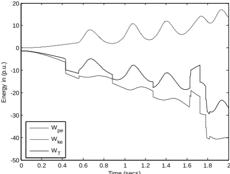
Case 1: Line (5, 7), t = 0.18sec, Unstable without HVDC

Figure. 4.2. Variation of Energy with time without HVDC

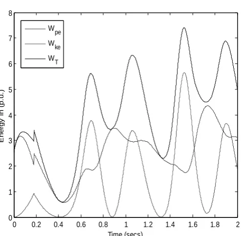
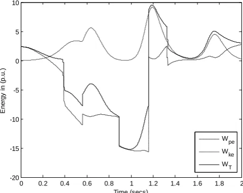
Case1: line (5, 7), t = 0.18sec, Stable with HVDC

Figure. 4.3. Variation of Energy with time with HVDC

0 0.2 0.4 0.6 0.8 1 1.2 1.4 1.6 1.8 2

-40 -30 -20 -10 0 10 20 30 40

Time (secs)

E

n

e

rg

y

i

n

(

p

.u

.)

W_pe

W_ke

W_T

0 0.2 0.4 0.6 0.8 1 1.2 1.4 1.6 1.8 2

0 1 2 3 4 5 6 7 8

Time (secs)

E

n

e

rg

y

i

n

(

p

.u

.)

W_pe

W_ke

Case1: line (5, 7), t = 0.18sec

Figure. 4.4. Variation of potential energy with time

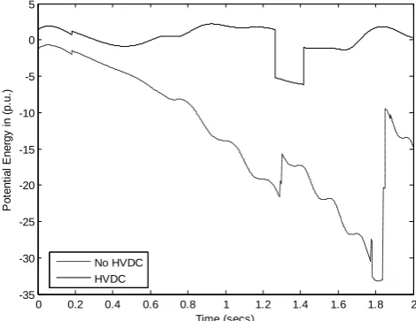
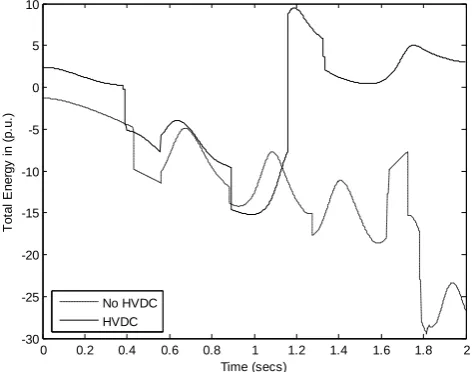
Case1: line (5, 7), t = 0.18sec

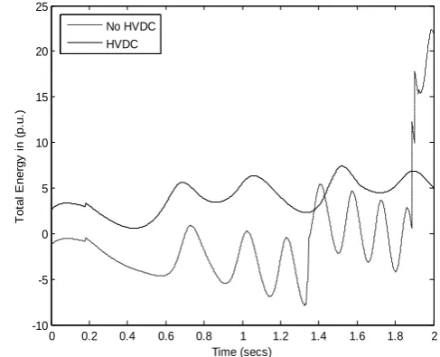
Figure. 4.5. Variation of kinetic energy with time Case1: line (5, 7), t = 0.18sec

Figure. 4.6. Variation of Total energy with time 0 0.2 0.4 0.6 0.8 1 1.2 1.4 1.6 1.8 2 -35

-30 -25 -20 -15 -10 -5 0 5

Time (secs)

P

o

te

n

ti

a

l

E

n

e

rg

y

i

n

(

p

.u

.)

No HVDC HVDC

0 0.2 0.4 0.6 0.8 1 1.2 1.4 1.6 1.8 2

0 5 10 15 20 25 30 35 40

Time (secs)

K

in

et

ic

E

ne

rg

y

in

(

p.

u.

)

No HVDC HVDC

0 0.2 0.4 0.6 0.8 1 1.2 1.4 1.6 1.8 2

-10 -5 0 5 10 15 20 25

Time (secs)

T

o

ta

l

E

n

e

rg

y

i

n

(

p

.u

.)

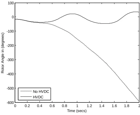
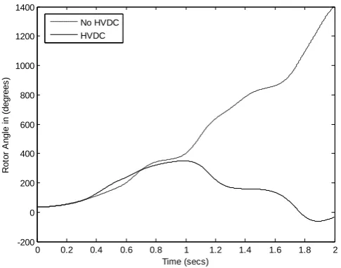
Case1: line (5, 7), t = 0.181sec of Machine-1

Figure. 4.7. Variation of Rotor angle with time

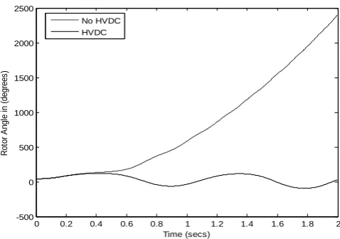
Case1: line (5, 7), t = 0.181sec of Machine-2

Figure. 4.8. Variation of Rotor angle with time

Case1: line (5, 7), t = 0.181sec of Machine-3

Figure. 4.9. Variation of Rotor angle with time 0 0.2 0.4 0.6 0.8 1 1.2 1.4 1.6 1.8 2 -600

-500 -400 -300 -200 -100 0 100

Time (secs)

R

o

to

r

A

n

g

le

i

n

(

d

e

g

re

e

s

)

No HVDC HVDC

0 0.2 0.4 0.6 0.8 1 1.2 1.4 1.6 1.8 2

-500 0 500 1000 1500 2000 2500

Time (secs)

R

o

to

r

A

n

g

le

i

n

(

d

e

g

re

e

s

)

No HVDC HVDC

0 0.2 0.4 0.6 0.8 1 1.2 1.4 1.6 1.8 2 -600

-500 -400 -300 -200 -100 0 100

Time (secs)

R

o

to

r

A

n

g

le

i

n

(

d

e

g

re

e

s

)

Case 2: Line (7, 8), t = 0.182sec, Unstable without HVDC

Figure. 4.10. Variation of Energy with time without HVDC

Case2: line (7, 8), t = 0.182sec, Stable with HVDC

Figure. 4.11. Variation of Energy with time with HVDC

Case2: line (7, 8), t = 0.182sec

Figure. 4.12. Variation of potential energy with time

0 0.2 0.4 0.6 0.8 1 1.2 1.4 1.6 1.8 2

-40 -30 -20 -10 0 10 20 30 40

Time (secs)

E

n

e

rg

y

i

n

(

p

.u

.)

W_pe W_ke W_T

0 0.2 0.4 0.6 0.8 1 1.2 1.4 1.6 1.8 2 -8

-6 -4 -2 0 2 4 6 8

Time (secs)

E

n

e

rg

y

i

n

(

p

.u

.)

W_pe W_ke W_T

0 0.2 0.4 0.6 0.8 1 1.2 1.4 1.6 1.8 2 -35

-30 -25 -20 -15 -10 -5 0 5

Time (secs)

P

o

te

n

ti

a

l

E

n

e

rg

y

i

n

(

p

.u

.)

Case2: line (7, 8), t = 0.182sec

Figure. 4.13. Variation of kinetic energy with time

Case2: line (7, 8), t = 0.182sec

Figure. 4.14. Variation of Total energy with time

Case2: line (7, 8), t = 0.183sec of Machine-1

Figure. 4.15. Variation of Rotor angle with time 0 0.2 0.4 0.6 0.8 1 1.2 1.4 1.6 1.8 2 0

5 10 15 20 25 30 35 40

Time (secs)

K

in

e

ti

c

E

n

e

rg

y

i

n

(

p

.u

.)

No HVDC HVDC

0 0.2 0.4 0.6 0.8 1 1.2 1.4 1.6 1.8 2

-10 -5 0 5 10 15 20 25

Time (secs)

T

ot

al

E

ne

rg

y

in

(

p.

u.

)

No HVDC HVDC

0 0.2 0.4 0.6 0.8 1 1.2 1.4 1.6 1.8 2 -600

-500 -400 -300 -200 -100 0 100

Time (secs)

R

o

to

r

A

n

g

le

i

n

(

d

e

g

re

e

s

)

Case2: line (7, 8), t = 0.183sec of Machine-2

Figure. 4.16. Variation of Rotor angle with time

Case2: line (7, 8), t = 0.183sec of Machine-3

Figure. 4.17. Variation of Rotor angle with time

Case 3: Line (4, 6), t = 0.56sec, Unstable without HVDC

Figure. 4.18. Variation of Energy with time without HVDC 0 0.2 0.4 0.6 0.8 1 1.2 1.4 1.6 1.8 2 -500

0 500 1000 1500 2000 2500

Time (secs)

R

o

to

r

A

n

g

le

i

n

(

d

e

g

re

e

s

)

No HVDC HVDC

0 0.2 0.4 0.6 0.8 1 1.2 1.4 1.6 1.8 2

-700 -600 -500 -400 -300 -200 -100 0 100

Time (secs)

R

o

to

r

A

n

g

le

i

n

(

d

e

g

re

e

s

)

No HVDC HVDC

0 0.2 0.4 0.6 0.8 1 1.2 1.4 1.6 1.8 2 -50

-40 -30 -20 -10 0 10 20

Time (secs)

E

n

e

rg

y

i

n

(

p

.u

.)

W_pe

W_ke

Case 3: Line (4, 6), t = 0.56sec, Unstable without HVDC

Figure. 4.19. Variation of Energy with time with HVDC Case 3: Line (4, 6), t = 0.56sec

Figure. 4.20. Variation of Potential energy with time Case 3: Line (4, 6), t = 0.56sec

Figure. 4.21. Variation of kinetic energy with time 0 0.2 0.4 0.6 0.8 1 1.2 1.4 1.6 1.8 2 -20

-15 -10 -5 0 5 10

Time (secs)

E

n

e

rg

y

i

n

(

p

.u

.)

W

pe

W

ke

W

T

0 0.2 0.4 0.6 0.8 1 1.2 1.4 1.6 1.8 2

-45 -40 -35 -30 -25 -20 -15 -10 -5 0 5

Time (secs)

P

o

te

n

ti

a

l

E

n

e

rg

y

i

n

(

p

.u

.)

No HVDC HVDC

0 0.2 0.4 0.6 0.8 1 1.2 1.4 1.6 1.8 2 0

2 4 6 8 10 12 14 16 18

Time (secs)

K

in

e

ti

c

E

n

e

rg

y

i

n

(

p

.u

.)

Case 3: Line (4, 6), t = 0.56sec

Figure. 4.22. Variation of Total energy with time Case 3: Line (4, 6), t = 0.57sec of Machine-1

Figure. 4.23. Variation of Rotor angle with time

Case 3: Line (4, 6), t = 0.57sec of Machine-2

Figure. 4.24. Variation of Rotor angle with time 0 0.2 0.4 0.6 0.8 1 1.2 1.4 1.6 1.8 2 -30

-25 -20 -15 -10 -5 0 5 10

Time (secs)

T

o

ta

l

E

n

e

rg

y

i

n

(

p

.u

.)

No HVDC HVDC

0 0.2 0.4 0.6 0.8 1 1.2 1.4 1.6 1.8 2

-600 -500 -400 -300 -200 -100 0 100

Time (secs)

R

o

to

r

A

n

g

le

i

n

(

d

e

g

re

e

s

)

No HVDC HVDC

0 0.2 0.4 0.6 0.8 1 1.2 1.4 1.6 1.8 2 -200

0 200 400 600 800 1000 1200 1400

Time (secs)

R

o

to

r

A

n

g

le

i

n

(

d

e

g

re

e

s

)

Case 3: Line (4, 6), t = 0.57sec of Machine-3

Figure. 4.25. Variation of Rotor angle with time

V.

CONCLUSION

In this paper, a technique is proposed for applying to the direct method of stability analysis to multi-machine AC/DC systems. A new method of handling transfer conductances is presented that is also useful in representing the DC link characteristics in the swing equations. The centre-of-angle formulation is used. A 3-machine, nine-bus system illustrates the validity of the method and the effects of the DC link in improving transient stability. Three case studies have been done and the computational algorithm and simulation results are presented.

VI. APPENDIX

Generator data: Base 100MVA Gen 1: 16.5/230 kv

Gen 2: 18/230 kv Gen 3: 13.8/230 kv Ka = 1.0 pu/rad per sec

Tdc = 0.1 sec

Pref = 0.0

Maximum Pdc = 2.0 pu

Minimum Pdc = -2.0 pu

qr = 0.5

REFERENCES

[1]. A.A. Fouad, “Stability Theory—Criteria for Transient Stability.” Proceedings of the Engineering Foundation Conference on System Engineering on Power, Henniker, New Hampshire, Publication No. CONF-750867, pp. 421-450, 1975.

[2]. T. Athay, R. Podmore, and S. Virmani, “A Practical Method for Direct Analysis of Transient Stability.” IEEE Transactions on Power Apparatus and System, vol. PAS-98, No. 2, pp. 573-584, 1979.

[3]. N. Kakimoto, Y. Ohsawa, and M. Hayashi, “Transient Stability Analysis of Electric Power System via Lure’ Type Lyapunov Function, Parts I and II.” Transactions of IEEE of Japan, vol. 98, No. 5/6, May/June 1978.

[4]. M. Ribbens Pavella, Lj T. Gruijc, T. Sabatel, and A. Bouffioux, “Direct Methods of Stability Analysis of Large Scale Power Systems.” Proceedings of the IFAC Symposium on Computer Applications in Large-Scale Power Systems, New Delhi, India, vol. II, pp. 168-175, August 1979.

0 0.2 0.4 0.6 0.8 1 1.2 1.4 1.6 1.8 2 -200

0 200 400 600 800 1000 1200 1400

Time (secs)

R

o

to

r

A

n

g

le

i

n

(

d

e

g

re

e

s

)

[5]. A. A. Fouad, and S. E. Stanton, “Transient Stability of a Machine Power System, Parts I and II.” Papers No. 81 WM 078-5 and 81 WM 079-3, IEEE Winter Power Meeting, Atlanta, Georgia, Feb. 1-6, 1981.

[6]. E. Uhlmann, “Stabilization of an AC link by a Parallel DC link.” Direct Current, vol. 12, No. 8, pp. 89-94, 1964.

[7]. H. A. Peterson, and P. C. Krause, “Damping of Power Swings in a Parallel AC and DC system.” IEEE Transactions on Power Apparatus and Systems, vol. PAS-85, pp. 1231-1239, 1966.

[8]. W. K. Marshall, K. R. Padiyar, L. M. Denton, W. J. Smolinski, and E. F. Hill, “ A Simplified HVDC Link representation for Stability Studies.” Paper C-74-434-7, IEEE Summer Power Meeting, July 1974.

[9]. M. A, Pai, M. A. Mohan, and J. G. Rao, “Power System Transient Stability Region Using Popov’s Method.” IEEE Transactions on Power Apparatus and Systems, vol. PAS-89, No. 5, pp. 788-794, May/June 1970.

[10]. J. L. Willems, and J. C. Willems, “The Application of Lyapunov Methods to the Computation of Stability Regions of Multi-Machine Power Systems, IEEE Transactions on Power Apparatus and Systems, vol. Pas-89, No. 5, pp. 795-801, May/June 1970.

[11]. J. L. Abatut and J. Fantin, “Etude de la Stabilite Transitoire dans un Systeme de Puissance Influence des Parametres.” Automatic Control Theory and Application, vol. 2, pp. 14-18, 1973.

[12]. H. Sasaki, “An Approximate Incorporation of Field Flux Decay into Transient Stability Analysis of Multi-Machine Power Systems by the Second Method of Lyapunov.” IEEE Transactions on Power Apparatus and Systems, vol. PAS-98, No. 2, pp. 473-483, March/ April 1979.

[13]. T. Athay, V. R. Sherkey, R. Podmore, S. Virmani, and C. Puech, “Transient Energy Stability Analysis.” Systems Engineering for Power: Emergency Operating State Control- -Section IV, U.S. Department of Energy Publication No. CONF-790904-PL, October 1979.

[14]. A. H. El-Abiad, and K. Nagappan, “Transient Stability Region of Multi-Machine Power Systems.” IEEE Transactions on Power Apparatus and Systems, vol. PAS-85, pp. 169-179, February 1966.

[15]. W. F. Tinney, and W. L. Powell, “The REI Approach to Power Network Equivalents.” 1977 PICA Conference, Toronto, Canada, May 1977.

[16]. P. M. Anderson, and A. A. Fouad, Power System Control and Stability. Ames, Iowa State University Press, 1977.

[17]. J. J. Dougherty, and T. Hillesland, “Power System Stability Considerations with Dynamically Responsive DC Transmission Lines.” IEEE Transactions on Power Apparatus and Systems, vol. PAS-95, pp. 536-541, March/April 1976.