High speed cameras for motion analysis in sports science

(1)

VOLUME 11 | ISSUE 1 | 2016 | 53

High speed cameras for motion analysis in

sports science

BASILIO PUEO 1

Sports Science, Faculty of Education, University of Alicante, Alicante, Spain

ABSTRACT

Pueo, B. (2016). High speed cameras for motion analysis in sports science. J. Hum. Sport Exerc., 11(1), 53-73. Video analysis can be a qualitative or quantitative process to analyze motion occurring in a single plane using one camera (two-dimensional or 2D) or in more than one plane using two or more cameras simultaneously (three-dimensional or 3D). Quantitative 2D video analysis is performed through a digitizing process that converts body segments or sport implements into digital horizontal and vertical coordinates in the computer. In order for these measurements to be accurate, image capture by means of video cameras must be sharp and motion blur-free, especially in high speed motions. In this paper, a detailed introduction to factors affecting image quality will be presented. Furthermore, selection of the most appropriate camera setting to undertake high speed motion analysis with the best quality possible, both spatially (focus and resolution) and temporally (frame rate, motion blur, shutter options and lighting), will be discussed. Rather than considering commercial criteria, the article will focus on key features to choose the most convenient model both from technical and economical perspectives. Then, a revision of available cameras on the market as of 2015 will be carried out, with selected models grouped into three categories: high-, mid- and low-range, according to their maximum performance in relation to high speed features. Finally, a suggested recording procedure to minimize perspective errors and produce high quality video recordings will be presented. This guideline starts with indications for camera selection prior to purchase or for testing if a given camera would fulfil the minimum features. A good video recording dramatically improves the analysis quality and enables digitizing software to produce accurate measurements. Key words BIOMECHANICS, PERFORMANCE, MOTION BLUR, SHUTTER SPEED, FRAME RATE.

1_{Corresponding author. University of Alicante, Faculty of Education, Ctra. San Vicente, s/n, 03080 Alicante, Spain}

E-mail: basilio@ua.es

Submitted for publication October 2015 Accepted for publication January 2016

JOURNAL OF HUMAN SPORT & EXERCISE ISSN 1988-5202 © Faculty of Education. University of Alicante

(2)

Photographic methods for the analysis of human motion began in 1878, when sequential pictures of galloping horses were taken as an experiment to check whether all four feet of a horse were off the ground at the same time while trotting. The use of motion picture cameras in human motion increased with the development of cinematography during the last century. Nowadays, miniaturization of computers and availability of technology have resulted in the widespread use of video cameras in any activity, including sport motion analysis (Wilson, 2008).

There are two types of video analysis: qualitative and quantitative. First, qualitative analysis of sport activities is the first and simplest way of evaluation since it is based on the criteria of the observer (subjective evaluation). As no absolute measurements can be retrieved from it, qualitative video analysis can be used to review executed motions which are too quick for the human eye or too complex to observe them at a glance. For example, an athlete can learn about proper technique in a relatively short time with qualitative video analysis techniques, such as slow motion or stop-action viewing (Garhammer & Newton, 2013). Second, the aim of quantitative motion analysis of sport and exercise activities by means of video recordings is to undertake a detailed analysis of subject’s movement patterns (Payton, 2008) and reduce injury risk (Bartlett, 2007). Although video cameras provide sequential two-dimensional images of movement at specific time intervals depending on the speed of the camera (McGinnis, 2013), quantitative analysis can be two-dimensional (2D) or three-dimensional (3D).

Initial quantitative analysis of human motion was 2D since it is a much simpler approach that assumes that movement is confined to a predefined plane or plane of motion. Some movement patterns have symmetries that permit to evaluate key aspects of 3D motion through a single 2D view. For example, in the analysis of walking gait, the most important parameters defining locomotion can be measured from a side 2D view (Garhammer & Newton, 2013). Taking accurate measurements from a single video camera view involves a precise procedure to minimize perspective error. There are complex activities involving movements in more than one plane, though, where a 2D analysis would not be able to accurately retrieve useful data. 3D coordinate data can be obtained if the motion is recorded by two or more cameras simultaneously, eliminating perspective error. These sets of synchronized points in space can be reconstructed into real-life 3D coordinates by means of the Direct Linear Transformation (DLT) method (Abdel-Aziz & Karara, 1971). This approach, also known as motion capture, involves more complicated video capture and analysis procedures and requires powerful computers and sophisticated software (Young et al., 2015).

(3)

VOLUME 11 | ISSUE 1 | 2016 | 55 Bavaresco, 2014). In addition, video analysis can be made with minimal interference with the performer, not only in controlled laboratories, but also outdoors or in real competitions.

In this paper, technical considerations for video cameras will be discussed, as the first and most important stage of quantitative 2D video analysis. The aim is to help sport scientists and coaches when selecting a video camera to undertake high speed motion analysis. Rather than considering commercial criteria, this paper is focused on key features to opt for the most convenient model both from technical and economical perspectives. Then, a selection of available cameras on the market will be revised in three groups of quality, paying special attention to maximum performance in relation to high speed features. Finally, a suggested data collection procedure to produce the best possible video recordings will be presented. A good video recording dramatically improves the analysis quality and enables digitizing software to produce accurate measurements.

FACTORS ON VIDEO QUALITY

In this section, factors that can degrade the quality of video image will be presented, particularly for sports science. They should be taken into account not only to classical video cameras but also to any device that can capture moving pictures to either store them in internal memory or transmit to a computer. Among them, we can find Digital Single Lens Reflex cameras (DLSR), Smartphone cameras, Videoconferencing USB or IP cameras.

Spatial Sampling

The main quality factor in spatial sampling is the resolving power, defined as the capacity of an instrument to produce separate images of closely placed objects (Davidson, Olenych, & Claxton, 2007). This list will cover both optical limitations due to the lens construction and sensor limitations due to image capture and resolution.

1. Focus

Focus is the ability of a lens to converge object points in the focal plane, where the sensor is located (Murphy, 2001). From practical point of view, lack of focus has an impact on the sharpness of details, which has a high relevance to sport analysis. Images out of focus are caused by aberrations of the lens.

Focal length is another specification of interest in lenses. Long focal length produces high magnification and narrow angle of view, whereas short focal length leads to negative magnification and wide angle of view. In practice, image is brought closer with long focal length (telephoto lens) and moved away with short focal length (wide-angle lens).

Lenses can have fixed or variable focus. A fixed-focus, fixed-focal length camera is the simplest camera for video analysis. If the subject is located where the focus is set, these cameras may be sufficient. For outdoors cameras, the subject should be distant since focus is set to infinity as factory default. However, for indoor cameras, such as fixed-focus webcams, the subject should be placed a few meters away for sharp images.

(4)

56 | 2016 | ISSUE 1 | VOLUME 11 © 2016 University of Alicante focusing in telephoto will always lead to a focused image in wide angle, whereas the contrary does not apply. If the subject is always at a fixed distance, it is advisable to lock the manual focus and focal length to the best value and avoid additional changes.

2. Optical and sensor resolution

Optical resolution describes the ability of a lens to distinguish small details of an object that is being imaged. When an image is in focus, it is the major factor of image resolution. Optical resolution is a function of the optical quality of the lens.

On the other hand, sensor resolution refers to the number of points of light (pixels) that are sampled within the sensor area and is commonly measured in megapixels. For a given sensor area, small pixels lead to high resolution. However, the smaller those pixels are made, the higher noise that sensor would give, limiting its use in low-light conditions. Resolution can be measured in digital imaging as an overall size of a picture counting pixels, giving rise to typical video resolution (pixels width x pixels height): Standard Definition SD 720x576 or 720x480 (depending on which SD format each country adopted), High Definition HD 1920x1080 or 1270x720 and Ultra High Definition UHD 3840x2160 for 4K and 7680x4320 for 8K. On the other hand, resolution can also be evaluated in lines, line pairs per millimeter (lp/mm) or spatial frequency response through the Modulation Transfer Function (MTF), also known as spatial frequency response (Boreman, 2001). This parameter is used to describe the quality of the image as the ability of the camera system to resolve detailed structures, resolution and contrast. Figure 1 shows the influence of resolution and contrast in two structures with different detail or spatial frequency.

Figure 1. Influence of resolution and contrast on different detailed images quality.

The MTF relates the contrast attenuation of white and black bands of decreasing width (more detailed) and fixed contrast when pass through the lens and is captured by the sensor. In this way, global MTF is the product of the MTF (quality) of individual parts of a camera, lens and sensor.

Temporal sampling

(5)

VOLUME 11 | ISSUE 1 | 2016 | 57

1. Frame rate

For video recording, frame rate is the number of images (frames) per second that a camera can capture, generally expressed in frames per second or fps. From a practical point of view, frame rate can be seen as individual pictures being taken per second

Table 1. Typical frame rates in fps for different cameras working in high definition (1280x720)

Frame rate Sample time Comments

24 fps 42 ms Film movies

48 fps 21 ms HFR movies (The Hobbit)

120 fps 8 ms High speed smartphones

240 fps 4 ms Typical max. fps action cameras

480 fps 2 ms Amateur max. fps with reduced resolution >1000 fps < 1 ms Professional high speed cameras

Our visual perception system is able to blend multiple images into a continuous moving picture with as little as 16 fps, as this is the threshold to which the mind no longer perceive sequences as flashing images. As it can be seen in Table 1, the standard rate for film was set as 24 fps, a value slightly above the perceptual limit. Advanced smartphones with slow motion capabilities can capture up to 120 fps with high definition formats, such as 1280x720. Sport action cameras, used in extreme sports for capturing wide-angle video of adventures, can typically capture up to 240 fps, although this value is expected to increase due to their popularity.

The lowest frame rate value is a slow sampling rate that can be used for notational analysis in most sports without loss of information. However, this frame rate is too slow for rapid objects such as projectile motions (throwing) and hits (balls, shuttlecocks, ice hockey pucks). In order to calculate how much a rapid object of the above moves between two consecutive frames, we have to know the transversal velocity (across the frame) and the frame rate used:

Distance moved = object velocity / frame rate

For example, consider a beach volleyball serve where the ball travels at 90 km/h (25 m/s). A camera with a frame rate of 240 fps would give:

Distance moved = 25 m/s / 240 fps = 10.4 cm

Therefore, in each frame time, the ball moves 10.4 cm, so the ball is sampled every 10.4 cm, which is an adequate limit for a 21 cm-diameter ball. If the same action is captured at 30 fps, the ball will be sampled as:

Distance moved = 25 m/s / 30 fps = 83.3 cm

(6)

2. Motion Blur

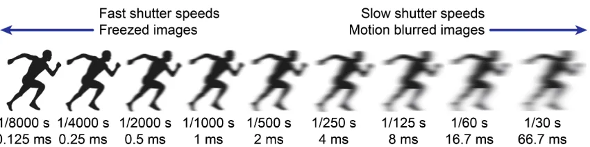
Motion blur is the appearance of smudges around the object and its path of movement. In films and regular recordings, motion blur is a natural effect that allows sampled moving images at discrete intervals to look as fluid sequences. However, in high speed situations, high frame rates may not be enough to freeze sudden movements due to motion blur. The main factors governing motion blur are object velocity and shutter speed, which is the time during which the sensor is exposed to light, measured in reciprocal second (Figure 2).

Figure 2. Video shutter speed values in reciprocal second and in absolute time.

In order to know if motion blur can pose a problem in frame-by-frame analysis, the camera shutter speed and the object velocity across the plane of interest must be known

Motion blur = object velocity x shutter speed

For example, consider again the beach volleyball serve where the ball travels at 90 km/h (25 m/s). A camera with a shutter speed of 1/1000 s would result in

Motion blur = 25 m/s x 1/1000 s = 2.5 cm

This value means that the ball will be blurred 2.5 cm, which is an adequate value considering the size of the ball. If we decrease four stops the shutter speed up to 1/250 s, motion blur will be:

Motion blur = 25 m/s x 1/250 s = 10 cm

(7)

VOLUME 11 | ISSUE 1 | 2016 | 59 Figure 3. Beach volleyball ball travelling at 90 km/h. (a) Still image, (b) Motion blur at 1/1000 s shutter

speed, (c) Motion blur at 1/250 s shutter speed.

In Figure 4, frame rate and shutter speed are combined for the examples above. Note that different number of sampled images can be acquired depending on the frame rate value for the first 70 ms of ball hit. A low frame rate of 30 fps would capture only three frames: at the beginning, at 83.3 cm and at 166.6 cm. Assuming that the ball spins while travelling, such frame rate would only capture it every 40 degrees, as depicted in the image. Alternatively, a moderate to high speed rate of 240 fps would capture one image every 10.4 cm, resulting in 17 images for the same time span. For this frame rate, the ball rotation can be analyzed with 5-degree resolution. Motion blur of 2.5 cm and 10 cm caused by 1/1000 s and 1/250 s shutter speeds, respectively, are the same for the two frame rate values. The resulting image can be seen in Figure 3.

(8)

60 | 2016 | ISSUE 1 | VOLUME 11 © 2016 University of Alicante Figure 4. Influence of frame rate and shutter speed values on a high speed recording of a beach volleyball serve at 90 km/h. Shutter speed values of 1/250 s and 1/1000 s for (a) frame rate 30 fps

and (b) frame rate 240 fps.

3. Shutter options

Shutter options are very important in Sports Science imaging applications since they set how and when light is captured during an exposure. In most digital cameras, the sensor determines the type of shutter electronically. Depending on the type of electronic shutter, an entire image can be captured at a single time or by scanning the scene in pixel rows or lines.

(9)

VOLUME 11 | ISSUE 1 | 2016 | 61 that all pixels are exposed at the same time, everything within each portion of frame determined by the shutter speed happens simultaneously. As a result, global shutters are typically considered as the best option to represent motion accurately.

The second type is the rolling shutter, where data is read out line by line from one side of the sensor to the other (usually horizontally). All the pixels in one row of the image collect data simultaneously and after a small delay, the next row is stored until the end of the image.

Figure 5. Shutter operation in the exposure of one video frame for rolling and global shutter technology.

Rolling shutters can cause some distortion effects, being wobble (also known as jello effect) the most important issue for high speed analysis. When the speed of the object is comparable to the delay between pixel rows, the object will be at slightly different positions from one line to another. This effect is noticeable with rotating objects at high speed (plane propellers for example) or when recording from a fast moving vehicle. Rolling shutter is used in most video cameras of the consumer market with CMOS sensors due to its ability to record in low light situations and the easy of construction. Figure 5 shows the two shutter technologies and the resulted image, with jello effect for the rolling shutter only.

4. Lighting

The ideal situation is to have high temporal sample rates (frame rate and shutter speed) to be able to capture many snapshots, all of them frozen in time to look still to analysts. However, camera specifications aside, every time the shutter speed is doubled, the exposure time for each frame is halved and therefore, the amount of light hitting the sensor is also halved. As a result, high temporal sample rates require great illumination of the subject.

(10)

Under these conditions, using faster shutter speeds becomes very difficult if the required amount of light must hit the sensor. For example, consider the beach volleyball serve that was successfully captured outdoors at 1/1000 s. If the recording takes place indoors with 1,000 lumens, the light level would be 100 times less than outdoors. To compensate for this light level drop, the camera must be operated to decrease 7 shutter speeds (log 100/log 2), from 1/1000 s to 1/8 s. As a result, the ball would be so blurred that no analysis would be possible:

Motion blur = 25 m/s x 1/8 s = 3.1 m

One way to override this limitation is to combine high sensibility of the sensor (high ISO number) and admit slightly dark videos due to underexposure to increase shutter speeds. The ISO number indicates how quickly a sensor absorbs light. For example, in the above situation, an increase in ISO number from 100 to 1600 would give 24 more sensibility to lighting (4 steps: 100-200-400-800-1600) and therefore the sensor would produce data image with 24 less light. Hence, shutter speed can be increased by 4 steps from 1/8 s to 1/125 s. In order to increase shutter speed, we can accept dimmer images up to 1/250 s.

This procedure has some drawbacks: high sensitivity leads to noisy images, also known as grain. Noise is observed in areas of color with speckled appearance instead of having a smooth look. Secondly, instead of exposing the sensor according to it sensitivity, an increase of one shutter speed means that half the light is hitting the sensor, leading to low brightness images. However, this dark video would still be useable for motion analysis with the advantage that motion blur will be adequate.

In order to increase the accuracy of observation and reduce motion blur even more, additional lighting must be set on the scene. The minimum floodlight number is one positioned perpendicular to the plane of performance, next to the video camera. This increases reflection from the subject, especially if there are retroreflective markers on the scene. Two additional light units can also be positioned at around 30º to the plane to avoid misunderstandings by shadows (Bartlett, 2007).

In high speed applications, the fluctuation or flickering of ballast-driven lights such as fluorescents or High-intensity gas discharge lamps (commonly known as HMI) must be considered before selecting the floodlight type (Box, 2010). Flickering is the subtle increase and fading in luminosity from light sources. One way of measuring the flickering effect is throughout the flicker factor, in the form of a number representing the maximum to minimum ratio of illuminance. A flicker factor of 0% means a constant flicker-free light, whereas 100% represents lighting vanishing entirely at its lower value or maximum flickering. Generally, a flicker factor of up to 3% is considered as flicker-free for general applications, including moderate high speed applications (Fuller, 2005).

(11)

VOLUME 11 | ISSUE 1 | 2016 | 63 Table 2. Summary of available light types for high speed applications.

Light type Advantages Disadvantages Flicker factor Sample

Tungsten – Inexpensive

– Brightness

– Minimal flickering

– Overheating

– Infrared radiation ––Tungsten lights: 0-10% House bulbs: 10-15%

–With dimmer: 50%

HMI – Good color

rendering

– Brightness

– Flicker at high fps –Electronic ballast: 0-3%

–Magnetic ballast: 40-70%

Fluorescent – Acceptable color rendering

– Brightness

– Efficiency

– Flicker at high fps –Electronic ballast: 0-12%

–Magnetic ballast: 30-60%

LED – Almost flicker-free

– Brightness

– Efficiency

– More expensive –Quality LED: 0-3%

–Low-cost LED: 0-15%

–On transformer: 40-70%

–Dimmed at 50%: up to 99%

Tungsten lights are considered as flicker-free due to inertia of the filament, although this is not entirely true so to low wattage lights. For example, household typical bulbs up to 100 W can produce significant flickering, especially if thyristor dimmers are used to decrease the amount of light.

HMI and other discharge lamps, like fluorescent lamps, usually operate on magnetic ballast, which cause high flickering factors between 30% and 70%. Special flicker-free electronic ballasts apply a transformation to decrease flickering between 1% and 3%. However, during lifetime, these figures usually increase up to the point where they are not advisable for high speed applications.

Finally, LED lights reacts very fast to changes in voltage, so the key in avoiding flickering relies on the power supply quality. Low-cost LED uses adapters to D.C. with significant ripples, similar to fluorescent, whereas quality adapters generate a stabilized voltage and therefore, without flickering. As with other light types, if dimmers are used, the benefits from the D.C. adapters vanish and massive flickering is displayed. Selection of the most appropriate flood light consists on finding a light source where the flicker frequency is higher than the frame per second value of the camera sensor. In this way, each frame would always capture a number of variations from maximum to minimum of light intensity, which will be recorded as a mean light value, rather than an alternate change.

CURRENT AVAILABLE CAMERAS

(12)

Table 3. Summary of available camera models distributed in three quality ranges.

Model Maximum _resolution rate at max. Max. frame resolution

Maximum

frame rate shutter speed Maximum Shutter type mount Lens

MSR price (Cost/frame @ 640x480)

Phantom Miro

LC320s 1920 x 1080 1,540 fps 8,490 fps @ 640 x 480 1/1000000 s (1us) (No jello effect) Global

Interchange F-, C-, PL and

EOS mount

$ 70,000 ( $ 8.22 )

Optronis

Camrecord 1000 1280 x 1024 1,000 fps 8,000 fps @ 1280 x 128 1/1000000 s (1us) (No jello effect) Global Interchange F-mount ( $ 12.7 ) $ 51,000

Edgertronic SC2 1280 x 864 2,797 fps 23,452 fps @ _{1280 x 96} 1/800000 s _(1.25us) _{(No jello effect)}Global Interchange _F-mount $ 10,000 _{( $ 2.0 )}

fps1000HD 1280 x 720 1,000 fps 4,000 fps @ _{640 x 360} 1/400000 s _(2.5us) _{(No jello effect)}Global Interchange _C-mount _{( $ 0.75 )}$ 2,300

Sony DSC-RX10 II 3840 x 2160 30 fps 1,000 fps @ _{1136 x 384} 1/32000 s _{(31.2 us)} Rolling shutter No _{( $ 1.4 )}$ 1,400

Casio EX-100F 1920 x 1080 30 fps 1,000 fps @ _{224 x 64} 1/10000 s _{(100 us)} Rolling shutter No _{( $ 5.0 )}$ 600

Sony Playstation

(13)

VOLUME 11 | ISSUE 1 | 2016 | 65 Table 3 presents a selection of currently available cameras, distributed into three user segments: high, mid and low range. It is precisely in the latter where lack of information is more evident, so analyst should evaluate carefully if they comply with expectations.

The first two cameras in Table 3 are sample models of the high-range cameras categories. These types of cameras are used for scientific, military, aerospace, automotive and research industries. In order to deliver high frame rates around 1,000-2,000 fps at high resolution, fast electronics and memory capabilities must be implemented. For example, when operating at maximum frame rate of 8,490 fps, 640x480 pixels, the camera must handle 2,600 million pixels per second information or 2.4 gigapixels per second (8,490x640x480/10243).

Another key feature is the shutter technology. All of them implement global electronic shutters on CMOS sensors, which allows for jello-effect-free images. Moreover, they deliver fast shutter speeds up to a 1 us (1/1000000 s) so motion blur is practically inexistent. These two features together force the rest of the device to implement high speed circuitry and communications. Therefore, these types of cameras can save the recorded data in high speed formats like SD cards and internal solid state drives (SSD) that provides transfer speeds of up to 1GB/second. Alternatively, some models are available with on-board memory, providing the capability of recording full 12-bit megapixel imagery for a few seconds.

Among other benefits, high range high speed cameras allows for the interchange of lenses of F-, C-, PL and EOS mounts. There are a vast variety of lenses available for these mounts, including photographic lenses, which exhibit low distortions and high resolution capabilities.

Finally, the main downside of this segment is the cost of the equipment. Cameras working in the vicinity of thousand fps at high resolution have a manufacturer's suggested retail price above $ 50,000, which prevents most sports science users to consider them for practical purposes. An interesting value to compare these and other quality-range cameras is the cost of each frame for a given resolution, which is 640x480 for this comparison. If a camera is able to deliver many frames per second at a low price, this value would be low, meaning that this model is cost effective. As seen in Table 3, high range cameras can be categorized between $ 5 and $ 15 per captured frame at 640x480. As it will be discussed later, not only high range cameras are the most expensive in terms of final price, but also in unitary price per frame.

The second group of cameras, named as mid-range in this paper, is an interesting alternative to the above owing to their high speed features at a reasonable cost for sports science analysts. In fact, they were born to offer cost-effective alternatives to high range models that can only be acquired by institutions with enough budgets, such as industrial or defense and aerospace research. The two models presented in Table 3 were funded by means of crowdfunding campaigns (Matter, 2015) with success, even though backers had to support the project with amounts around $ 5,000. Hence, there was a market niche that these campaigns have covered to try democratizing the use of high quality low cost cameras in many applications, including motion analysis in sports science.

(14)

model, the maximum resolution and frame rate of 4,000 fps at 640 x 480 indicates that internal circuitry and communications must be of high quality to transfer data at rates of 1,220 million pixels per second information or 1.1 gigapixels per second. These two models are in the price range between $ 2,000 and $ 10,000, which is a fraction of the first two cameras discussed above. This price difference can be seen in the unitary price per frame of $ 2 for the Edgertronic model and $ 0.75 for the fps1000HD model in comparison to the range of $ 5 and $ 15 for high range cameras. Differences in unitary price between Edgertronic and fps1000HD aside, both models deliver between enough frame rate and shutter speed values for HD video to cover almost every high speed situation in sports sciences. For the high-speed features at reasonable price, this camera range can be considered as low cost.

Finally, the consumer market has brought with models aiming at shooting high speed videos for amateur purposes. There is very large range of available models with different frame rates and even some smartphones has low motion recording, which is an alternative way of stating high speed video. Manufacturers claim these high speed features to attract consumers, but they do not display key features for sports science in technical specifications because it does not boost sales.

The main missing piece of information is whether the camera is operating with automatic or manual exposure. In auto exposure mode, the camera will pick a shutter speed according to available light, usually with exposure times too long to freeze moving images. Although high shutter speeds may be advertised in some models, if they operate in auto mode, the resulting shot will be at unknown shutter speed for the user.

As of late 2015, only two camera models are available offering full manual control of shutter speed values. The first one is the Casio EX-100F, substituting the well-known first affordable high speed camera Casio FH100, discontinued some years ago. The EX-100F delivers 30 fps at HD 1920x1080 video, intended for regular use. Several high speed modes are available with increasing fps and decreasing resolution, from 240 fps at 640x480 to 1,000 fps at 224x64. Manual shutter speeds up to 100 us (1/10000 s) can be selected by user, regardless of the high speed mode selected. All models from this range of cameras are equipped with rolling shutter, which may have jello effect in rapid movements and mount fixed lens. The latter is usually not a problem owing to different fields of view (FOV) that zoom lenses offer to users.

A recent model by Sony with manual shutter speed is able to capture 4K video (3840x2160) at 30 fps. Such bandwidth is associated with fast electronics, allowing high speed modes from 250 fps at 1824x1026 to 1,000 fps at 1136x384. Shutter speeds are also better than the previous model, up to 31.2 us (1/32000 s). Larger zoom aside in this model, both cameras have the same drawbacks of jello effect and fixed lens. Although the DSC-RX10 II is about twice the MSR price as the Casio model, the unitary cost per frame is very low, about $ 1.4, owing to high speed and high resolution combined together.

(15)

VOLUME 11 | ISSUE 1 | 2016 | 67 RECORDING GUIDELINE

In this part, the above information will be revised to make a practical guideline for recording quality high speed video with enough resolution and minimal motion blur for accurate analysis.

Camera selection

Selection of frame rates and shutter speeds are a function of object motion to be recorded. Each sport is characterized by a particular range of motion velocities, from minimum velocity, sometimes null, to a maximum velocity. For example, in a beach volleyball serve, there can be many parts to track: from ball at 90 km/h maximum speed that will decrease with distance, hand in contact with the ball at 60 km/h to maximum jump vertical speed of 11 km/h of the player. This velocity range of around 80 km/h may change the camera requirements depending on the purpose of analysis. In general, the highest velocities of body parts are not the fastest values. Sport implements, such as rackets or golf clubs, together with ball hits, are the fastest motions under analysis.

Table 4. Velocities of sports projectiles and recommended high speed camera settings.

Sport _(cm)D _(m/s)Vm fpsm _(cm)dm SS_(s)m _(cm)MBm _(m/s)V∞ fps∞ _(m/s)d∞ SS_(s)∞ MB_(cm)∞

Badminton 6.0 137 1000 14 1/10000 1.4 6.7 60 11.1 1/480 1.4

Tennis 6.5 73 480 15 1/4000 1.8 22 180 12.2 1/1500 1.5

Ping-pong 4.0 32 480 7 1/4000 0.8 10 120 8.3 1/1000 1

Squash 4.0 78 1000 8 1/8000 1 34 180 7.1 1/3200 1.1

Jai alai 6.5 83 640 13 1/4000 2 41 320 13 1/2000 2

Golf 4.2 91 1000 9 1/8000 1.1 48 480 10 1/4000 1.2

Volleyball 21 37 100 37 1/800 4.6 20 48 42 1/400 5

Football 21 51 120 42 1/1000 5.1 30 75 40 1/500 6

Softball 9.7 47 240 19 1/2000 2.3 33 180 18.3 1/1500 2.2

Baseball 7.0 54 480 11 1/3000 1.8 40 320 12.5 1/2000 2

Cricket 7.2 53 480 11 1/3000 1.8 40 320 12.5 1/2000 2

Lacrosse 6.3 50 480 10 1/3000 1.7 48 400 12 1/3000 1.6

Handball 19 27 75 36 1/600 4.5 36 100 36 1/800 4.5

Basketball 24 16 48 33 1/250 6.4 31 75 41 1/500 6.2

D: Diameter, Vm: Fastest speed, fpsm: Frame rate for Vm, dm: Distance moved for fpsm, SSm:

Shutter Speed for Vm, MBm: Motion Blur for SSm, V∞: Terminal velocity. The same applies for

the remainder variables with ∞ subscript.

Diameter and velocity data extracted from (Clanet, 2015). Rest of data computed by the author according to the following criteria: fps is chosen so that dm and d∞ equals 2*D and

shutter speed is chosen so that MBm and MB∞ equal 25% of D.

Table 4 shows a quantitative representation of the sport projectiles that have spherical symmetry (balls) or cylindrical symmetry (shuttlecock), with two characteristics velocities: the highest recorded speed of the

(16)

From a practical point of view, these sport projectiles start at maximum velocity to slow down up to terminal speed in which ball’s trajectory will depend on speed, aerodynamics and gravitation (parabola, straight path, knuckleball, tartaglia curve, spiral and pop-up) (Clanet, 2015).

For both Vm and V∞, the recommended frame rate and shutter speed values are calculated according to

maximum distance moved and motion blur. First, minimum frame rate is selected so that ball travels twice its diameter at most, giving enough spatial information for a proper analysis of the ball trajectory. With such frame rate, no more than the size of the ball will separate two consecutive snapshots, as depicted in Figure 6(a). Second, as discussed above, minimum shutter speed is selected so that maximum motion blur is 25% of ball diameter, which allows analysts to make accurate readings and ball tracking in digitizing software. The maximum visualized ball diameter will be 1.25 times the real diameter, as shown in Figure 6(b). These criteria are used to calculate the minimum frame rates and shutter speed values for a range comprising maximum velocity, usually at the beginning of the projectile motion, to terminal velocity, when particular trajectories are produced.

Figure 6. Maximum distance moved between frames (a) and maximum motion blur (b) as criteria to estimate recommended minimum frame rate and shutter speed values, respectively.

Geometric setup

The above maximum velocities can then be used to estimate a range of track velocities with corresponding frame rate and shutter speed parameters. However, the object velocity may be different from the recorded velocity depending on the camera position with regards to the plane of motion (PoM). Therefore, three practical cases can be found.

a) Plane of motion perpendicular to the camera viewing direction (lens axis).

(17)

VOLUME 11 | ISSUE 1 | 2016 | 69

b) Plane of motion parallel to the camera viewing direction (lens axis).

This is the opposite case, where objects move toward or away from the camera. Projected velocity on the sensor will be null, so no motion blur is expected. Only in extremely fast objects, such as shuttlecocks travelling directly towards the lens of a camera, velocity will be captured as a slight increase in size. However, even in these situations, motion blur is negligible.

This view is not very common for biomechanics analysis, in which projected velocity must be as similar as possible as the object itself to give accurate readings. However, when the aim of analysis is not the moving object but manifestations in other planes, such view is adequate. For example, the trajectory of a tennis ball after hitting the net can be observed by placing the camera parallel to the net, with the lens towards the ball.

c) Plane of motion at other angles with respect to camera viewing direction (lens axis).

This view encompasses all other directions not covered in the above views. The plane of motion is neither perpendicular nor parallel to the camera viewing direction, so an angle is formed between them. Therefore, the projected velocity on the sensor will be the velocity in the plane of motion multiplied by a projection factor (cosine of angle between plane of motion and sensor). Since this factor is always less than one, the recorded velocity will be less than the real velocity in the plane of motion.

Projected velocity = MoP velocity x cos (angle between sensor and MoP planes)

Figure 7. Camera positions and estimated velocity from recordings.

Figure 7 depicts the three cases described above for a football kick of 100 km/h. When captured with the camera viewing direction perpendicular to the PoM, the captured velocity is 100 km/h (case a) and on the other hand, when the camera lens is in the ball axis, velocity is null (case b). At other angles, for example, at 30 degrees from the plane of motion, the captured velocity will be:

(18)

In this case, frame rates and shutter speeds must be selected according to projected velocity, less than MoP velocity, so less motion blur is expected. If the aim is to calculate the real MoP velocity from observations, readings must be corrected by dividing from the same factor:

MoP velocity = Projected velocity / cos (angle between sensor and MoP planes)

In this case,

MoP velocity = 86.6 km/h / cos 30 = 100 km/h

However, although this setup is beneficial to minimize issues related to camera high speed capabilities since projected velocity values are lower than those of MoP, the observed velocity is very inaccurate because it is a projection different of that of interest. This inaccuracy increases with angle up to 90 degrees, where situation b) is reached.

Frame rate and shutter speed selection

Once the highest velocity of interest has been selected, whether from body parts or implements, or whether actual PoM or projected, estimate the two parameters needed for high speed video.

a) Calculate the minimum frame rate for a maximum distance of the moving part between consecutive

frames

Min. frame rate = object velocity / max. distance moved

Therefore, selected frame rate should be higher than the resulting value to have enough frames covering the entire movement. As a rule-of-thumb, the maximum distance between frames should be twice the size of the projectile size in the plane of motion. For example, consider football ball travelling at 28 m/s (100 km/h); if we want to capture a frame every 42 cm (2*D), frame rate should be higher than 67 fps, so the camera should work at 75 fps.

b) Calculate the minimum shutter speed for a maximum motion blur in each frame

Min. shutter speed = object velocity / max. motion blur

(19)

VOLUME 11 | ISSUE 1 | 2016 | 71 DISCUSSION

In selecting high speed cameras, the first decision would be regarding the aim of the recording. For attractive videos, typically viewed in slow motion, there is no need to worry about issues discussed here, like motion blur or rolling shutter. In fact, minimizing motion blur can make videos more disturbing to public as almost all audiovisual input, like movies, are recorded with blurred motion paths, so human vision is expecting some motion blur to decode motion correctly. For example, graphic designers add certain amount of blur to synthetic images created by computer to give a more realistic sensation of movement. On the other hand, frame-by-frame analysis needs always as low motion blur as possible.

In order to minimize motion blur and have enough spatial information, or frames per second, there are more and more high speed cameras on the market. As of 2015, most of the so claimed high speed models have automatic exposure control, which means that shutter speed is selected automatically as a function of unknown criteria, such as actual illumination, sensitivity (ISO) settings, etc. Thus, the shutter speed offered by the camera is not selected to minimize motion blur, but to give bright and clear images. Although alternative shutter speeds might have been selected, resulting in dimmer images but with less motion blur, the internal camera algorithm will provide blurred images.

To make things even worst, internal algorithms driving to specific shutter speed values or range of shutter speed values used for certain modes are not public, preventing users from making predictions on the amount of motion blur. Generally, it is straightforward to find frame rate values and image resolutions for high speed video since manufacturers use this information as a plus to aid sales. However, some other key features for frame-by-frame analysis are more difficult to find, sometimes hidden within particular working modes or named with commercial definitions. For example, information about manual exposure and/or automatic exposure, total recording time (some ultra-high speed cameras can only record a few seconds), type of image compression, etc. Finally, photographic cameras that also work in video mode may lead to confusion when revising specifications. It is common to find very interesting features like high shutter speeds, but these specifications are often not clear if they apply only to photography mode or also to video modes.

Most of the high speed camera reviews published on internet or magazines are focused on features for the general public, such as image resolution. There are certain camera models with manual shutter speed control that are not reviewed because the resolution they offer is below to qualify for a review. Therefore, sport analysts may have difficulties in selecting models to minimize motion blur. Another source of information would be internet videos by owners. Typically, review videos of new camera models made by amateurs try to show attractive scenes like water drops, from which motion blur is not displayed properly to evaluate its impact on image.

(20)

images. Although not particularly unpleasant in typical attractive videos from these cameras, for quantitative motion analysis of sport, in which kinematic information (linear and angular position, velocity and acceleration of body segments and implements) is to be retrieved, such distortion makes them not advisable.

CONCLUSIONS

High speed video cameras are one of the most important piece of equipment that every sport scientist or coach can use to analyze athletic motion in training and competition. Although high speed capture technology has made a huge progress in last years, there has been no democratization for analysts who want to control their specifications manually. These limitations prevent users from unwanted side effects, such as the jello effect or motion blur distortions.

Despite these limitations, high speed cameras can be regarded as one of the most versatile tools for frame-by-frame analysis of athletic motion. Current technology allows engineers to design camera systems with manual control for users to take control of the take, all at reasonable prices. However, the camera market is full of high speed models with basic features that only satisfy recreational or attractive videos. For athletic motion analysis, manufacturers must include full manual control of some specific features related to the sensor shutter since they are paramount of how each tiny instant of time is captured. It is therefore necessary that sport scientists and coaches know the underlying technology inside a high speed camera to further demand manufacturers with affordable equipment for quality videos.

REFERENCES

Abdel-Aziz, Y., & Karara, H. M. (1971). Direct Linear Transformation from Comparator Coordinates into

Object Space Coordinates in Close-Range Photogrammetry. American Society of Photogrammetry,

81(2), 1–18.

Balsalobre-Fernández, C., Tejero-González, C. M., del Campo-Vecino, J., & Bavaresco, N. (2014). The Concurrent Validity and Reliability of a Low-Cost, High-Speed Camera-Based Method for Measuring the Flight Time of Vertical Jumps. Journal of Strength and Conditioning Research, 28(2), 528–533. Bartlett, R. (2007). Introduction to Sports Biomechanics. Sports Biomechanics.

Boreman, G. D. (2001). Modulation transfer function in optical and electro-optical systems. SPIE Press. Box, H. C. (2010). Set lighting technician’s handbook  : film lighting equipment, practice, and electrical

distribution. Focal Press.

CL Eye. (2014). Retrieved October 5, 2015, from https://codelaboratories.com/products/eye/ Clanet, C. (2015). Sports Ballistics. Annu. Rev. Fluid Mech, 47, 455–78.

Davidson, M., Olenych, S., & Claxton, N. (2007). Photomicrography, in Focal Encyclopedia of Photography, (4th ed.). Focal Press.

Fuller, P. W. W. (2005). Some Highlights in the History of High-Speed Photography and Photonics as

Applied to Ballistics. In High-Pressure Shock Compression of Solids VIII (pp. 251–298).

Berlin/Heidelberg: Springer-Verlag.

Garhammer, J., & Newton, H. (2013). Applied Video Analysis For Coaches: Weightlifting Examples. International Journal of Sports Science and Coaching, 8(3), 581–594.

Matter, M. (2015). edgertronic slow-motion video camera. Retrieved October 2, 2015, from http://wiki.edgertronic.com

(21)

VOLUME 11 | ISSUE 1 | 2016 | 73 Payton, C. (2008). Biomechanical Evaluation of Movement. Sports Biomechanics.

Spivak, A., Kumar, A., & Franchetti, M. (Eds.). (2013). Energy Assessments for Industrial Complexes. Bentham Science Publishers.

Wilson, B. D. (2008). Development in video technology for coaching. Sports Technology, 1(1), 34–40. Young, W., Dawson, B., Henry, G., Young, W. B., Dawson, B., & Henry, G. J. (2015). Sports Science &