Prediction of nominal strength of composite structure open hole specimen through cohesive laws

(1)

Abstract—the nominal strength of open hole specimens has a

great intense in composite material industry. The physical cohesive laws between the crack opening displacement and the cohesive stress over length of fracture processing zone FPZ are used to imply the nominal strength. The result is a valuable graph that relates the nominal strength with respect to the crack

size and FPZ length ℓ_{. The nominal strength of quasi-brittle}

structures has been analyzed taking into account the geometry and size of the specimen and the shape of the cohesive law. Simple design tables for a constant and linear cohesive law have been developed. Furthermore, the procedure to compute the nominal strength with a general bilinear cohesive law is defined.

Index Terms—Nominal Strength, cohesive law, FPZ, notch

Strength, un-notch strength.

1 INTRODUCTION

Numerous efforts have been made to find out the notched strength of laminated composites containing through the thickness discontinuities. Waddoups et al. [1] have modulated Linear Elastic Fracture Mechanics LEFM for the notched composite materials. Wu [2] has formulated a failure criterion and established that crack propagation was characterized by failure within a critical volume. The size effect on structural strength refers to the modification of nominal strength with respect to the dimension of the structure while keeping constant the geometrical proportions and the material. Quasi-brittle structures (or materials) experiments a decreasing of the nominal strength and increasing of brittleness with respect to the increase of structural dimension. The source of size effect law is the development of a stable failure process zone FPZ. The Size effect Law SEL was initially derived for notched structures through the R curve [3]. The SEL is:

(1)

Mohammed. K. Hassan is with the South Valley University, Qena, Egypt, 83521 (corresponding : [email protected];).

Y. Mohammed, is with the South Valley University, Qena, Egypt, 83521 (corresponding [email protected];).

T. M. Salem is with is with Minia University, Faculty of Engineering, Egypt.

A. M. Hashem Hassan is with the South Valley University, Qena, Egypt, 83521 (corresponding :[email protected];).

Where A is dimensionless constant, D is characteristic dimension of structure or specimen, Do is constant with length

dimension and

σ

_u

is un-notch nominal strength. SEL is obtained through asymptotic matching of the two extreme responses of the structure. Forming two limits; the first limit is a plastic limit which is for small sizes whereas the LEFM is considered the second limit for large sizes. Taking into account this two extreme responses eqn. (1) can be completely adjusted with two geometric and two material parameters. Plastic limit is obtained for small specimens (D→0) when the stress at failure plane is constant and equal to the material strength. The nominal strength can be written as: σ N = Aσ u = βP σ u, where βP depends exclusively on the specimen geometry. For large sizes ((D→∞)) the nominal strength is obtained by LEFM. The parameter (D0 = βFMβP-2χ), where (χ = EGc/σu2)- Irwin’s characteristic length[3]- and βF is a geometric parameter that can be obtained through the stress intensity factor. Modifications of the size effect for notched structures are done [4], that accounts are more precisely for the size effect law for relatively small structures [5].

Materials as concrete, composites, toughened ceramics among others are Considered as quasi-brittle materials. Due to the industrial importance of laminated composite materials some models have been developed to obtain the nominal strength of open hole OH specimens. The point stress method PSM and the average stress method ASM [6], assumes that the failure stress occurs when the stress or average stress over some distance away from the discontinuity is equal to the un-notched material strength, this distance is assumed material property independent of geometry, this has no physical meaning. The inherent flaw method IFM [1] assumes that a critical crack of length a0 is present in the material. The length of this inherent flaw is determined by means of the un-notched strength as: _a _K 2 _{/ (} ₎

u

o = _C π σ .

Srivastav [7] modified the PSM criteria using expression of Tan [8] for characteristic length as it was assumed a function of size of the hole as well as aspect ratio:

( / )n( / )s

d_o = m a a_r b a , but with considering that m and n are constant for a particular material and for particular width of the plate where (a, half of the hole size, ar, reference hole size, b=a, Aspect ratio, m, n and s are the constants for a -1/ 2

1 - D

u _D

σ σ

ο

 

= Α  

Ν _ _

Prediction of nominal strength of composite

structure open hole specimen through cohesive

laws

(2)

International Journal of Mechanical & Mechatronics Engineering IJMME-IJENS Vol: 12 No: 01 2

particular material) but again the characteristic length expression is of no physical meaning.

The cohesive stress is assumed as a material property that defines the stress with respect to the crack opening. The process presented can be related back to Dugdale [9] on yielding of steel strip, where the failure stress is assumed as function of the length of the FPZ for sharp crack and a constant cohesive stress. The work of Dugdale had been generalized to linear or bilinear cohesive laws and to other specimen geometries as compact tension or open hole specimen [10].

The aim of this paper is to relate the nominal strength of

open hole specimen composite laminates with the stable FPZ

length

FPZ

l

using different types of cohesive laws not only

the constant one but also linear, exponential, and bilinear laws comparing their obtained results. The paper methodology is as follow; in first section the process of derivations is defined, and in the next section the definition of cohesive laws are presented. In the last section the failure strength of open hole specimen is calculated with the help of the available cohesive laws. The validity of the results is analyzed by experimental results the importance of the shape of the cohesive law is analyzed by comparing the different nominal strength obtained by materials with the same characteristic parameter ρcr and θW.

, l , ,

R c r F P Z

w _W c r _R _R

R R F P Z

θ ρ θ

λ

= = =

= ₊

l l

l

(2)

Where R is open hole radius W is composite plate width, and

lcr

is characteristic length and

λ

is characteristic parameter.

The main goal of the present paper is to find the

normalized nominal strength (or the nominal stress concentration factor):

1 N

S_N K _N

u σ

σ −

= = (3)

Where_S

N is normalize nominal stress,

σ

N

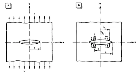
notch nominal strength.

2 Cracked hole specimen

It will consider a plat with finite width having an open hole (stress raiser), this hole will be assumed as a pre crack of a length (2a) that equal diameter of the open hole (2R). It will be replaced by a total effective crack of length 2d, where d=R+ℓ, (see Fig. 1). Such that:

1. A constant stress

σ

is applied over the FPZ length (ℓ) where a<χ<d

2. d is selected in such a manner that

∑

K

=

0

or

s

K

= −

K

_σ

This problem is solved by superposition method and by assuming there is certain point load P applied at a distant χ from the center of an element has width wi=b2-b1.

Fig. 1. Cracked Plate

The concentrated force

p

=

σ

(

b2 b1

−

)

at χ =b.where

(

2 1

)

b

=

b

+

b / 2

.To resume the solution, the length (ℓ=d-R) of FPZ is determined as mentioned before by superposition

method, the stress intensity factor,

K

_total, at the ends of the damage zone is zero.

total s

K

=

K

+

K

_σ (4)

Where

K

_s and

K

_σ are the stress intensity factors for a crack emanating from each side of the hole due to the remote stress S and local stress σ, respectively.

The stress intensity factor due to remote applied stress S is;

2

1 1 2

R

K

_s

d F F

N

_W

σ





π

=



−







(5)

Where

σ

_N is the mean stress at failure plane, Rhole radius, W specimen width, and F1, F2 is hole, width correction factors respectively shown in appendix.The remote applied stress

2

1

N

R

S

W

σ





=



−







The stress intensity factor for crack emanates from hole with length ℓ for constant crack face stress profile.

2 1

1 1

2 d sin b sin b _{3 4}

K F F a

d d

σ

=

_π

 −  − −   =

   

 

(3)

If the stress in the failure process zone is not constant, (see Fig. 1b), and decartelized in n steps (as piecewise constant) the stress intensity factor can be approximated as:

1

1 n

n

K

a

i

i i

i

σ

=

∑

=

∑

=

(7)

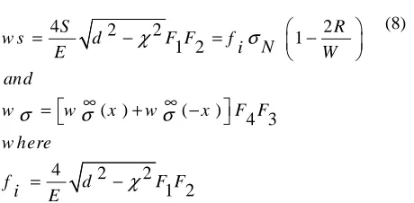
The crack opening displacement is obtained by means of the equations:

4 ₂ ₂ 2

1 1 2

( ) ( ) _{4 3}

4 2 2

1 2

S R

w s d F F f

N i

E W

and

w w x w x F F

w here

f d F F

i _E

χ

σ

χ

  = − =  −    ∞ ∞   =_ + − _ = −

Where the total crack opening can be computed as:

total s

w

=

w

+

w

_σ (9)

Where F3 and F4 is the partially loaded hole width correction factors respectively and wσ shown in appendix. While in case of the stress in the failure process zone is not constant, the displacement Wi at a point χ i in the damage zone due to a unit

stress

σ

_i over a loading element i.

w

w s

w

total

i

and

w

i

ij

σ

σ α σ

=

+

=

(10)

Where A( , ) A( )

ij i j i j

α

=

χ χ

+⇒ _{− +}

χ

isinfluence

function, for ,j=1,…..n. see appendix

3 COHESIVE LAWS

The behavior of crack is defined by the relationship between the cohesive stresses and the relative displacement (w) between the upper and lower face which known by softening function. The cohesive zone model

alternative method (with respect to the classical fracture mechanics) to study the crack propagation in materials. It differs from the others because it purposes distribution of the energy needed to propagate the crack. This

shape is called cohesive law and depends of certain parameters that are unique for each material Fig. 2. The constant stress, linear and exponential cohesive laws are widely used because only requires two well-known material properties to b If the stress in the failure process zone is not constant, (see

steps (as piecewise constant) the stress intensity factor can be approximated as:

The crack opening displacement is obtained by means of the

4 2 1 S R E W   = − =  −    (8)

Where the total crack opening can be computed as:

is the partially loaded hole width correction shown in appendix. While in case of the stress in the failure process zone is not constant, the in the damage zone due to a unit

isinfluence

The behavior of crack is defined by the relationship between the cohesive stresses and the relative displacement (w) between the upper and lower face which known by cohesive zone model CZM is an alternative method (with respect to the classical fracture mechanics) to study the crack propagation in materials. It differs from the others because it purposes distribution of the energy needed to propagate the crack. This distribution or shape is called cohesive law and depends of certain parameters that are unique for each material Fig. 2. The constant stress, linear and exponential cohesive laws are widely used because known material properties to be

adjusted. Unfortunately, these cohesive laws do not offer enough exibility to be adjusted to most of the materials of interests. A bilinear cohesive law as shown in Fig. 2.d has been used to adjust the response of concrete [11] and laminated composite materials [12].

Fig. 2. Different form of cohesive laws

3.1 GENERALIZATION COHESI

The Dugdale work on yielding of steel strip is generalized to open hole specimen. This model assumes constant relation between crack face stress and crack opening displace

The profile of crack opening is related with the stress profile

by the operator

f

ij

=

i

β

j

+

α

ij

with the stress profile with the cohesivelaw length of the FPZ when the crack opening profile is

decartelized in n steps, the crack opening at position i can be related with the stress at position j of the FPZ with an expression of the form:

(

_j

)

W

f

w

i

=

ij

σ

j

That gives the crack opening profile and combined with the cohesive law gives the stress profile. With Eqns.

nominal strength is defined by equation. 1

1

2 ₁ ₁

sin sin

2 1

n

N _i i i

p w here

c b F F

i i

i _d _d _{F F}

R p _W σ β σ β β π β = ∑ =  ₋   ₋   = −  _ _− _ _        = −

To determine the ℓMax that produces the maximum nominal strength it is necessary to solve:

/

N

σ

∂

l

3.2 IMPLEMENTATION OF THE

The numerical implementation of the cohesive laws will be solved using M. file written by Matlab code 2010.

4 NOMINAL STRENGTH

For a given relative length of the eqn. (11) gives the stress profile at the

the nominal stress is obtained. The relative length of the at failure load is obtained by eqn.(13).

adjusted. Unfortunately, these cohesive laws do not offer enough exibility to be adjusted to most of the materials of interests. A bilinear cohesive law as shown in Fig. 2.d has been used to adjust the response of concrete [11] and

Fig. 2. Different form of cohesive laws

ENERALIZATION COHESIVE LAW

The Dugdale work on yielding of steel strip is generalized to open hole specimen. This model assumes constant relation between crack face stress and crack opening displacement. The profile of crack opening is related with the stress profile

ij

i

j

ij

and the crack opening with the stress profile with the cohesivelaw σ(w). For a given length of the FPZ when the crack opening profile is

elized in n steps, the crack opening at position i can be related with the stress at position j of the FPZ with an

(11)

That gives the crack opening profile and combined with the cohesive law gives the stress profile. With Eqns. 4, 5 and 6 the nominal strength is defined by equation.

1 1 3 4

1 2

c b F F

i i

d d F F

    

 _ _ _ _

    

 

(12)

Max that produces the maximum nominal strength it is necessary to solve:

(13)

MPLEMENTATION OF THE COHESIVE LAWS

The numerical implementation of the cohesive laws will be

Matlab code 2010. OMINAL STRENGTH

(4)

4.1 TWO PARAMETERS COHESIVE LAWS

The constant, linear and exponential softening laws shown in Figs. 1.a, b and c are the most common two parameters cohesive laws. For constant cohesive law, the nominal strength is obtained when the maximum crack

opening displacement reaches

W

C _;

C C

u

G

W

=

_σ

, and the condition expressed in Eqn. 13 is reached. In this paper the experimental data were taken from reference [10] and listed in table 1

Table 1 Fracture properties and geometry of the used composite laminates [10].

E11,GPa

C

G

kj/m2

σ

_u,MPa

85 37 810

4.1.1CONSTANT COHESIVE LAW

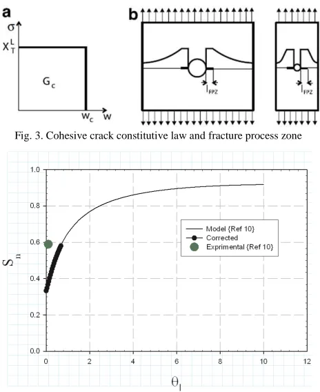
The maximum load is obtained with respect to the length of the cohesive law according to eqn. (13). The softening curve and stress distribution profile are shown in Fig. 3. The crack opening profile is defined by equation (11). The maximum load is obtained when the maximum crack opening is reached

C

W

;

G_C W_C

u σ

=

where Wi = Wc. applying general nominal stress eqn. (12) with ci = d and bi = R and σi = σ u the result is thenominal strength according to constant cohesive law extracted from the generalized law form.

Fig. 3. Cohesive crack constitutive law and fracture process zone

Fig. 4. R-curve of laminated Plate predicted by constant cohesive law

Fig. 5. Nominal Strength sensitivity predicts by constant cohesive law composite laminated plate

u i

N _p

β σ

σ = _β (14)

The relation plot between length of fracture process zone FPZ, ℓFPZ at any time and nominal stress is shown in Fig. 4.

It is clear from the figure that the constant cohesive law predicts that the plastic limit is reached and FPZ occupies all the fracture planes. But this is not the true because the area under the softening curve (R-curve) shown in Fig.4 must be equal to the surface fracture energy G1C for mode I. so the critical crack opening should be taken into account. Therefore it should be cut off at FPZ when Wi = Wc this is calculated by eqn. (13) with respect to eqn. (11) as shown in Fig. 4.

It is shown in Fig. 5 that as the hole diameter increases the notch strength decreases due to stress concentration factors and FPZ increment. The Results are between plastic and elastic limits curves. As the composites laminates is qusti-brittle materials, some extreme values are known as follow If

cr

ρ

_→∞_then 1

(1

_w

)

_w

θ

_{= −}

θ θ

−

l and SN = 1 that

corresponds to the plastic limit and if

ρ

_cr

=

0

then

θ

l=0 and

1

( )

N t

S

=

K

−

w

which corresponds to the elastic limit.

Fig. 6. Stress concentration factor

(5)

{

}

1 2

(

)

2 ₁

1 sin

( )

3 4

F F

K

_t

_w

F F

θ

λ

π

=

−

(15)

4.1.2LINEAR COHESIVE LAW

The FPZ in this case is represented as the normal traction σ on the crack flanks decreases linearly with the crack normal displacement 2 w the linear cohesive law shown in Fig.2 b is expressed by the eqn. (16):

1

2 u w

i

u

i

G

C

σ

 

 

 

=

−

(16)

With eqns. 11 and 16 an expression of the form is obtained: 1

1 W

C

W f I

C

i _u ij ij

σ _σ δ 

 

 

−

= +

(17)

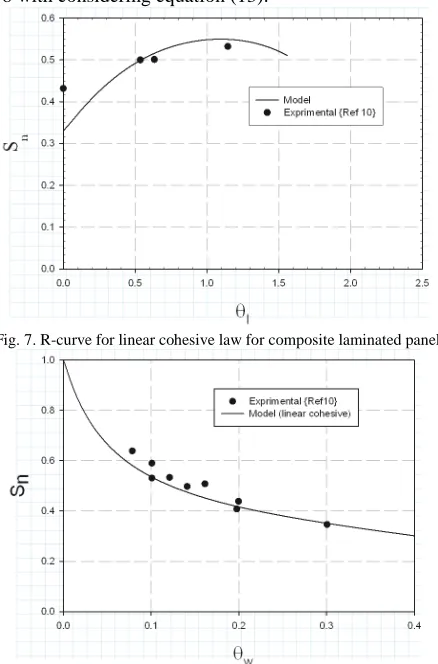
The R curve for composite laminates is predicted successfully by this form as shown in Fig.7. The model underestimates the stress at the crack initiation but predicts the critical length and the tensile nominal strength successfully. The linear cohesive form is predicts the crack sensitivity very well as shown in Fig. 8 with considering equation (13).

Fig. 7. R-curve for linear cohesive law for composite laminated panel

Fig. 8. Nominal Strength sensitivity predicts by linear cohesive law composites laminated plate

4.1.3EXPONENTIAL COHESIVE LAW

The exponential cohesive law shown in Fig.2c is expressed by the eqn.:

exp( u wi)

u

i _Gc

σ

=

σ

− (18)

With eqn. 11 and equation (18) solved numerically it can obtained an expression of the form:

( )exp( )

, u j

w f _w w

i ij l _Gc

σ

θ θ

= − (19)

The solution of this equation with respect to eqn. (13) for maximum crack length at failure load predicts R-curve and the crack size sensitivity (see Fig.9 and Fig.10).

Fig. 9. R-curve for exponential cohesive law for composite laminated panel

Fig.10. Nominal Strength sensitivity predicts by exponential; cohesive law laminated plate

Again as in the linear cohesive law the model underestimates the stress at the crack initiation, predicting the critical length and the tensile nominal strength successfully. Whereas, it predicts the crack sensitivity lightly successful compared with previous law because the area under softening curve GC is less than the same area in previous ones.

4.2 FOUR PARAMETERS COHESIVE LAWS

(6)

concrete or laminated composites. The softening function will be approximated by a bilinear function Fig.1 d. This simple diagram captures the essential facts: large scale debonding, or fracture of aggregates in the steepest part, and frictional pull-out of aggregates in shallow tail of the diagram. This function is completely characterized when the following four parameters are known as shown in Fig. 1 d: tensile strength σu and Gc and two more parameters, these can be two of the: H0;HF; rσ; rw;wc or the center of masses of the cohesive law: ww or σw(see Fig.11) .

Fig. 11 Bilinear cohesive law

4.2.1 BILINEAR COHESIVE LAW

For a four parameters cohesive law it is possible to construct a normalized nominal strength as before but with two more variables involved. A characteristic of most of the materials is that the slope at the beginning of the cohesive law is greater than the slope at the end. For these materials the maximum load is obtained with a small opening besides the hole. The shape of a bilinear cohesive law shown in Fig.11 can be expressed with the function [14]:

-( )

( - )

H w w r w

u o w f

w

H w w r w_w w w

f f f f

σ





<

= _{< <} (20)

Where H0 is the slope of the first line, HF is the slope of the second line. wf is the opening in which no stresses are transferred to the crack faces and rw is the ratio of the crack opening at intersection point.

; 2

2 (1 )

; ;

2

2 (1 ) R rw r

G_c _uR r

w Ho

f _uR G r_c _w

Rr u H

f G_c _rw σ

σ

_σ

σ

_σ

= +

−

= =

= ₋

(21)

The center of masses of the cohesive law: 2

1

( )

3( )

0

w c

w

f r_w r r_w r

w w w dw w

f

G

σ

r_w

σ

r

_σ

σ

+ +

= ∫ = ₊

(22)

0

1

( ) ( )

3( )

u

w w u

c w

r r r r

w w d

G r r

σ

σ σ

σ

σ = σ σ σ = + + σ

+

∫

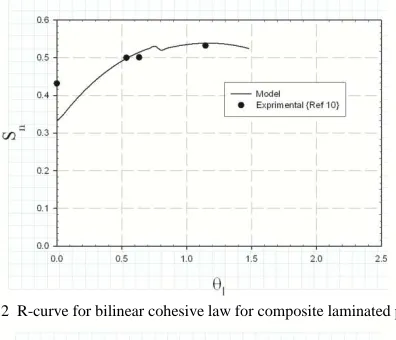
(23)

Considering eqns. 20, 21 with eqns. 11 and 12 the R-curve can be extracted as shown in Fig. 12 which fitted the experimental data of reference [10]. Applying Eqn. 13, notch sensitivity curve is constructed Fig. 13. These curve is agree very much with the experimental data this because the long tail of the bilinear cohesive law.

Fig. 12 R-curve for bilinear cohesive law for composite laminated panel

Fig. 13 Nominal Strength sensitivity predicts by bilinear; cohesive law for laminated plate

4.2.2 ADJUSTMENT OF BILINEAR COHESIVE LAW

The adjustment of the cohesive law requires four parameters. The material strength: σu, which can be measured with a tension specimen for the advanced materials or for more "random" materials as concrete the Brazilian test. The total fracture toughness: Gc, measured from the propagation of a crack in a sufficiently large fracture mechanics specimen. The last parameter is the displacement centroid of the cohesive law ww that is determined from the long tail of the load-displacement curve of a notched beam test [15- 17]. Dvila et al. [12] adjust a bilinear cohesive law to compact tension specimen made of CFRP cross ply laminate composite.

4.2.3 GENERALIZATION BILINEAR COHESIVE LAW

(7)

Table 2 shows different cohesive law shapes.

# rw rσ R

C1 0.25 0.25 0.5

C2 0.5 0.5 1 linear

C3 1 1 2 constant

5 COMPARSION LAWS

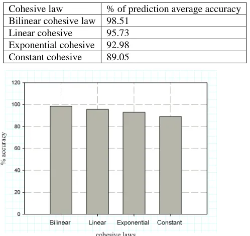
The various types of physical cohesive laws are shown in the previous Figures. In order to investigate the accuracy degree of each one, Fig. 14 reveals a comparison among them. This comparison shows that, the prediction of SN using constant cohesive law is the highest one. This is because of the natural assumed relation between the nominal displacement and the normal traction is surrounding all the laws and the linear surrounding the exponential whereas the four parameter cohesive law bilinear cohesive law fit displays a much longer tail than other two parameter cohesive law (Wc = Wf = 2GC/σ) while in bilinear (Wf = 2GC/σ R), However the initial line of the bilinear cohesive law is very close to the other cohesive law this explained the good fit of two parameter cohesive law for the experimental results. This as far as the peak load is concerned and long as the specimens are not too large. This is illustrated in Fig. 15. Fig. 16 and table 3 show the average percent of accuracy for each laws respect to experimental results in [10], it is found that the bilinear cohesive law is the best one to give good fit for nominal strength for the previous reason.

Fig. 14 comparing physical cohesive laws

Fig. 15 curve tail of different cohesive law

Table 3 cohesive laws accuracy percent

Cohesive law % of prediction average accuracy Bilinear cohesive law 98.51

Linear cohesive 95.73 Exponential cohesive 92.98 Constant cohesive 89.05

Fig. 16 Accuracy for different cohesive laws

6 CONCLUSION

Influence of the cohesive law in the nominal strength is analyzed and the differences on the nominal strength are quantified. It must be concluded:

• The shape of the cohesive law is important to precisely define the nominal strength of quasi-brittle materials that dissipates under intrinsic mechanisms.

• To take into account the influence of the cohesive law it is required to take into account the interaction of the FPZ in the elastic response of the structure. Therefore it is not possible to detect the influence of the shape of the cohesive law without the functions of the stress intensity factor and crack opening.

(8)

APPENDIX

A. Correction factors

A.1 Remote applied Stress [10]:

The circular hole and finite width correction factors F1 and F2 are given:

2 3 4

1

2

1

(1 0.35 1.425 1.578 2.156 ) 1 sec sec 2 2 (1 ) w w F F where λ λ λ λ λ πθ π θ λ λ θ − = + + − + −     =        

= + l

(A.1)

A.2Partially loaded crack

The circular hole and finite width correction factors F3 and F4 are given:

( , ) 3

1 2 1 1 sin sin

/ 1

3 ₁ (4 ) ₂

1 2 1 2

( , ) 1 sin 1

2 2

1 2(1 ) (1 ) 2(1 ) _/

2

2 4

0.02 0.558 1

2 4

2 0.221 0.046

1 1

sin ₂ sin ₁ 4 G F b b d d b d

A A A A

G b d A A B B F γ λ γ γ γ λ γ γ λ λ λ λ _γ λ λ λ λ =  ₋  ₋  −  _ _ _ _        =    −    ₋  =+ ₋ +  + ₋ +  −  − −           ₌ = − + = + − ₋ − = sec 2 2 1

sin 1 sin 1

. sin 2 1, 2 sin 2 d

b b w

d d where b i w Bi i d w π π π            _ _ _ _ _ _  ₋_ _₋ ₋_ _      _ _ _ _           = _ _ =     (A.2)

B. Crack opening displacement

The approximate crack surface displacement for partially loaded crack is given by:

( ) ( )

2 2 ₍ _{) cosh} 1 2 2 2_sin 1

1

w w w

b b

d b _b

w b d

E d b d

b b χ χ σ σ σ χ σ _χ _χ σ π χ        _ _    _ _  _ _     ∞ ∞ = + − = − ∞₌ ₋ − ₊ ₋ − − ₌ (B.1)

When the traction along the crack faces is represented in a piecewise constant fashion the displacement ws for remote applied stress at the midpoint of each loading elements χi is:

2 1 2 2 / 2 ( ) s i i S

w d F F

E where i R l n

χ

= − −   = + −    l l (B.2)

The function A(χi,χj) is given by equation B.1 with b1=bj and b2=cj for j=1,2,…..,n. for plane stress A is:

2

( , ) ( )cosh12 ( )cosh12 sin1 sin1

2 3 4

i j

A E

d c d b c b

j i j i j j

c b d F F

j i _d _c j i _d _b i d d

i j i j

χ χ π χ χ χ χ χ χ χ                =  _ _ _ _ __               − − − − − − − − − + − − − − (B.2)

F1, F2, F3 and F4 are the same like in A.1 and A.2 but with b1 and b2 replaced by bi and ci, respectively, where:

( ) 1 ( ) i i i c R n i b R n = + − −   = + −    l l l l (B.3) ACKNOWLEDGMENT

Y. Mohammed acknowledges the AMADE research group in Girona university Spain for their help in this research during my scholarship.

REFERENCES

[1] M. E. Waddoups, J. R. Eisenmann, B. E. Kaminski, Macroscopic fracture mechanics of advanced composite materials, Journal of Composite Materials 5 (1971) 446-454.

[2] E.M. Wu, in: L.J. Broutrnan (Ed.), Fracture and Fatigue, Technomic Publishing Company, Stamford, 1974, p. 157.

[3] Z. P. Bazant, J. Planas, Fracture and Size Effect in Concrete and Other Quasi-brittle Materials, CRC Press, Boca Raton, Florida, 1998.

[4] J. Planas, G. V. Guinea, M. Elices, Generalized size effect equation for Quasi-brittle materials, Fatigue and Fracture of Engineering Materials and Structures 20 (5) (1997) 671-687

[5] Y. N. Li, Z. P. Baznt, Eigen-value analysis of size effect for cohesive crack model, International Journal of Fracture 66 (3) (1994) 213-226

[6] J. M. Whitney, R. J. Nuismer, Stress fracture criteria for laminated composites containing stress concentrations., Journal of Composite Materials 8 (1974) 253-265. [7] V.K. Srivastava, Notched strength prediction of laminated

composite under tensile loading Materials Science and Engineering A328 (2002) 302–309

[8] S.C. Tan, J. Comp. Mater. 21 (1987) 949.

[9] D. S. Dugdale, Yielding of steel sheets containing slits, Journal of the Mechanics and Physics of Solids 8 (2) (1960) 100-104.

[10] C. Soutis, N. A. Fleck, P. A. Smith, Failure prediction technique for compression loaded carbon fiber-epoxy laminate with open holes, Journal of Composite Materials 25 (11) (1991) 1476-1498.

[11] G. V. Guinea, J. Planas, M. Elices, A general bilinear fit for the softening curve of concrete, Materials and Structures 27 (2) (1994) 99-105.

[12] C. G. Davila, C. A. Rose, P. P. Camanho, A procedure for superposing linear cohesive laws to represent multiple damage mechanisms in the fracture of composites, International Journal of Fracture 158 (2) (2009) 211-223. [13]Walter D. Pilkey, Peterson's Stress Concentration Factors,

(9)

[14] P. Maimì, A. Sharma, The role of the shape of the cohesive law in the size effect of open hole tension specimens, AMADE, Escola Politµecnica Superior, Universitat de Girona, Girona, Spain, (2009).

[15] G. V. Guinea, J. Planas, M. Elices, Measurement of the fracture energy using three-point bend tests: Part 1-influence of experimental procedures, Materials and Structures 25 (4) (1992) 212-218.

[16] J. Planas, M. Elices, G. V. Guinea, Measurement of the fracture energy using three-point bend tests: Part 2-influence of bulk energy dissipation, Materials and Structures 25 (5) (1992) 305-312, .