Design of a New Area Control Error Based Load Frequency Controller for a Two-Area Interconnected Power System

(1)

76 Abstract—Successful operation of an interconnected power system requires the matching of total generation with total demand and associated system losses. With time as the operating point of a power system changes, and hence, these systems may experience deviations in nominal system frequency and scheduled power exchanges to other areas, which may yield undesirable effects. The two variables are considered for the evaluation of the system performances namely, frequency and tie-line power exchanges. In this two-area symmetrical thermal reheat system with stiff and elastic tie lines are considered for simulation controllers using proportional and integral are designed and the simulated results are analyzed for better performance.

Index Terms—Area Control Error, Load Frequency Control, Settling Time, Stiff tie-line, Elastic tie-line.

I. INTRODUCTION

Recently, the evaluation of control performances of interconnected power systems has become an important issue with respect to individual load frequency controls. In this paper the system performance is evaluated using the settling time based stability criterion in a two-area thermal reheat power system interconnected with elastic and stiff tie-lines. The design of controllers with proportional and integral are implemented and the simulated response for change in output frequency, tie-line power flow and input power are analyzed with the mathematical model developed for a two area symmetrical thermal reheat power system, interconnected with stiff tie-line and elastic tie-lines. The results reveal that the system with elastic tie-line ensures better transient response and less settling time.

Manuscript received November 20, 2010

R. Arivoli is with the Department of Electrical Engineering,Annamalai University,Annamalainagar–608002,Tamilnadu,India(lnrarivolizc@yahoo. co.in).

G. Gurumoorthy is with the Meenakshi Sunararajan Engineering College, Chennai,India.([email protected])

Dr. I.A. Chidambaram, is with the Department of Electrical Engineering, Annamalai University, Annamalainagar–608002, Tamilnadu, India(e-mail: [email protected]).

II. TWO AREA SYSTEM MODELS

A. System model with stiff tie-line

This model is based on the assumption that transmission lines within each individual control area, and tie lines between areas, are completely stiff, Then, the whole system can be characterized by a single frequency. That is, all the generators of the system swing in unison [2].

The real power deviation, ΔPI_i, of the interchange between area i and the rest of areas in the system, can be obtained from the dynamic equation of the generators and the fact that the overall exchange balance between areas must be zero.

The model proposed in fig.1 can be improved by introducing the load-frequency characteristic of the areas in the dynamic equation of the power system and representing in more detail the speed governor and the turbine-generator of the power plants. Then, assuming neglected line losses, the deviation of interchanged real power can be written as

F

Δ

)

β

-α

( ) 2 PD

Δ

-2 PG

Δ

( -)

α

-1 )( 1 PD

Δ

-1 PG

Δ

( = 2 PI

Δ

= 1 PI

Δ

Where ΔPG_i is the incremental power generation of area i,

i PG

Δ is the increment of load consumption in the area, and β

α, are coefficients given by

Design of a New Area Control Error Based Load

Frequency Controller for a Two-Area

Interconnected Power System

First R. Arivoli, Second G. Gurumoorthy, Third Dr. I.A. Chidambaram

ΔP

+ +

ΔPI1(S ΔPI2(

1+sT

(2)

77 ) 2 ( ) 2 D + 1 D ( 1 D = β ) 1 ( 2 r P . 2 H + 1 r P . 1 H 1 r P . 1 H = α ) 3 ( 2 = n p sT + 1 p K = ∑n 1 =

i (ΔPGi ΔPDi) ) s ( F Δ 2 1 1 2 1 2 . 2 2 1 ` . 1 2 * 1 D D p K D D r P H r P H F p T + Δ + + Δ

F* being the rated frequency.

B. System model with elastic tie-line

The two-area system model with elastic tie-lines is based on the assumption that transmission lines within each individual control area are strong in relation to ties between areas[2]. So, a whole area can be characterized by a single frequency. This implies that generators belonging to an area swing in unison but on necessarily with generators of the other area.

Neglecting line losses, the increment tie-line power,

,

PI

Δ

can be written as

) 2 1 ( * 12

12 T f dt f dt

PI = ∫Δ −∫Δ Δ

Where cos(₁* ₂*)

12 | 2 | 1 | 2 *

12 Δ δ −δ

X V V T

is the synchronizing coefficient or electrical stiffness of the tie-line; X12, its reactance and

V

_i

=

|

V

_i

|

e

jαi the bus voltage

of the line terminal i.

Fig.2. Interconnected with elastic

tie-KI1

1+sT

+ - ΔPG1(s 1+sTG1

ΔPD1(s

ΔPI12(s

1+sT 1+sTKP2P

Power

III. PERFORMANCE EVALUATION

A. Area Control Error (ACE)

Generally, it is assumed that the characteristics of the load fluctuations are the same in the two control areas and there is no correlation between the load fluctuations of each control

area, each standard deviation of the load fluctuations is proportional to the square root of the system capacity. If each control area’s governor response and LFC contribute equally, the standard deviation of ACE should be proportional to the square root ratio of its capacity divided by the total capacity of interconnected power systems [1].

The permitted values of the standard deviation of ACEs are expressed as given below

) 4 ( ) REF ( ACE σ P / A P ≤ A ACE σ ) 5 ( ) REF ( ACE σ P / B P ≤ B ACE σ

Supposing the averages of ACEA and ACEB are 0, their

sample variances will be expressed by the following equations. ) 6 ( ∑ N ₂ A ACE σ = 2 A ACE N 1 ) 7 ( ∑ N ₂ B ACE σ = 2 B ACE N 1

Then the sample variance of ACE of whole system can be expressed as follows.

∑ +

= N ACE_A ACE_B N ACE 2 ) ( 1 2 σ ) 8 ( AB ACE R 2 + 2 B ACE σ + 2 A ACE σ =

Where = ∑NACE_AACE_B N

AB ACE

R 1

Substituting (4) for (8), (8) and can be expressed as

AB ACE R REF ACE P B P REF ACE P A P ACE 2 2 ) ( 2 ) ( 2 + + ≤ σ σ σ AB ACE R REF ACE 2 2 ) ( + ≤σ

When there is no correlation between the ACEs, the standard deviation of the ACE of whole system should become less than the permitted value.

IV. SIMULATION RESULTS

The optimum value of integral controller gains the two-area Interconnected thermal reheat system with stiff tie-line were found to be K_i_stiff₁ =0.3;K_istiff₂ = 0.3and that for

(3)

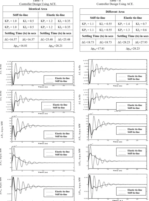
78 Table - I

Controller Design Using ACE. Identical Area

Stiff tie-line Elastic tie-line

KP1 = 1.0 KI1 = 0.5 KP1 = 1.2 KI1 = 0.35

KP2 = 1.0 KI2 = 0.5 KP2 = 1.2 KI2 = 0.35

Settling Time (ts) in secs Settling Time (ts) in secs

Δf1=16.57 Δf2=16.57 Δf1=25.48 Δf2=25.48 Δptie=16.81 Δptie=28.21

0 5 10 15 20 25 30

-0.025 -0.02 -0.015 -0.01 -0.005 0 0.005 0.01 0.015 0.02

Tim e (s)

0 5 10 15 20 25 30

-0.025 -0.02 -0.015 -0.01 -0.005 0 0.005 0.01 0.015 0.02

Tim e (s)

0 5 10 15 20 25 30

-2 0 2 4 6 8 10 12 14 16

x 10-3

Tim e (s)

0 5 10 15 20 25 30

-5 0 5 10 15

x 10-3

Tim e (s)

0 5 10 15 20 25 30

-0.02 -0.01 0 0.01

Tim e ( s )

Fig (3). Frequency Deviations, Control Input Deviations and Tie-Line Power Deviation of a Two area Power System( Identical areas) Interconnected with

Elastic and Stiff tie-lines for 1% Step Load Change in Area 1.

Table - II

Controller Design Using ACE.

Different Area

Stiff tie-line Elastic tie-line

KP1 = 1.1 KI1 = 0.55 KP1 = 1.4 KI1 = 0.7

KP2 = 1.1 KI2 = 0.55 KP2 = 1.3 KI2 = 0.6

Settling Time (ts) in secs Settling Time (ts) in secs

Δf1=18.73 Δf2=18.73 Δf1=28.23 Δf2=27.93 Δptie=17.81 Δptie=28.23

0 5 10 15 20 25 30

-0.025 -0.02 -0.015 -0.01 -0.005 0 0.005 0.01 0.015

Tim e (s)

0 5 10 15 20 25 30

-0.025 -0.02 -0.015 -0.01 -0.005 0 0.005 0.01 0.015

Time (s)

0 5 10 15 20 25 30

-2 0 2 4 6 8 10 12 14 16

x 10-3

Tim e (s)

0 5 10 15 20 25 30

-5 0 5 10 15

x 10-3

Tim e (s)

0 5 10 15 20 25 30

-0.02 -0.01 0 0.01

Tim e ( s )

Fig (4). Frequency Deviations, Control Input Deviations and Tie-Line Power Deviation of a Two area Power System( Different areas) Interconnected with

Elastic and Stiff tie-lines for 1% Step Load Change in Area 1.

∆

PTie

in p.

u.

M

W

∆

PC2

in p.

u.

M

W

∆

PC1

in p.

u.

M

W

∆

f2

in Hz

∆

f1

in Hz

……… Elastic tie-line

______ Stiff tie-line

______ Stiff tie-line ∆ P

Tie

in p.

u.

M

W

∆

PC2

in p.

u.

M

W

∆

PC1

in p.

u.

M

W

∆

f2

in Hz

∆

f1

in Hz

(4)

79 V. CONCLUSION

Load frequency control models of interconnected power system with elastic tie-line representation enables a clear improvement upon models with stiff tie-line. In fact elastic tie-line models provide more detailed information about the system evolution of the frequency of each individual control are and the power interchanged through each tie-line. Evaluation of control performances of interconnected power system of two-area with stiff and elastic tie-lines were simulated by designing the proportional plus integral controllers. Simulated results reveal that better performance can be achieved when the two-area power system inter connected with elastic tie-lines. More over, combination of stiff and elastic tie-lines can also be incorporated to have a better performance in inter area power flow.

REFERENCES

[1] Tetsuosasaki, KazuhiroEnomoto, “Statistical and Dynamic Analysis of Generation control performance standards”, IEEE Transactions on Power Systems, pp. 100-105, 2001.

[2] L.Basanez, J.Riera and J.Ayza, “Modelling and simulation of Multiarea Power System Load frequency Control”, Mathematics and computers in Simulation, pp. 54-62, 1984.

[3] Ibraheem, Prabhat Kumar, and Dwarka P. Kothari, “Recent Philosophies of Automatic Generation Control Strategies in Power Systems”, IEEE Transactions on Power Systems, vol.20, pp.346-357, February 2005.

[4] R.N.Patel, “Application of Artificial Intelligence of Tuning the Parameters of an AGC”, Internal Journal of Mathematical, Physical and Engineering Sciences, vol.1, pp.34-40, 2007.

[5] I.A. Chidambaram and S.Velusami, “Decentralize Biased Controllers for Load-Frequency Control of Interconnected Power Systems Considering Governor Dead Band Non-Linearity”, IEEE Indicon 2005 Conference, Chennai, India, pp.521-525, 11-13 Dec. 2005.

[6] Nasser Jaleeli and Louis S.VenSlyck, Priority-based Control Engineering (PCE) Dublin, Ohio “NERC’S new Control Performance Standards”, IEEE Transaction on Power Systems, pp.1092-1099, vol.14, No.3, August 1999.

[7] Subrata Mukhopadyyay, “Modern power system control and operation”,Rorrkeee publishing house, pp.174-176, 1983.

[8] Hadi Saadat, “Power system analysis”, WCB McGraw-Hill pp.542-555, 1999.

[9] K.Ramar and S.Velusami, “Design of decentralized load-frequency controllers using pole placement technique”, Electric Machines and Power Systems, vol.16, pp.193-207, 1989.

[10] Naotoyorino, yoshifumi, Koichinakanishi, Satonikona Kagawara, Yoshifumikamei and Hiroshisasaki, “Features Extraction of AR as a performance Index for Load frequency controls of Interconnected power Systems”, Electrical Engineering in Japan, vol.154, No.1, pp.20-26, 2006.

APPENDIX – A

A.1 Data for the interconnected two area(Identical) thermal power system [ 5]

Rating of each area = 2000MW. Base power = 2000 MVA. fº = 60Hz.

R1 = R2 =2.4Hz/p.u.MW.

H1 = H2 =5Sec.

Tg1 = Tg2 =0.08sec.

Tr1 = Tr2 =10Sec.

T11 = T12 =0.3sec.

Kp1 = Kp2 =120Hz/p.u.MW.

Kr1 = Kr2 =0.5.

Tp1 = Tp2 =20sec.

β1 = β2 =0.425p.u.MW/Hz.

T12 = 0.0707 p.u.MW/Hz.

a12 = -1.

∆Pd1= 0.01 p.u.MW.

∆Pd2= 0.0 p.u.MW.

A.2 Data for the interconnected two- area(Different) thermal power system [15]

Rating of each area = 2000MW. Base power = 2000 MVA. fº = 60Hz.

R1 = 2.4Hz/p.u.MW.

R2 = 5Hz/p.u.MW.

H1 = 5Sec.

H2 = 5Sec.

Tg1= 0.08sec.

Tg2= 0.25sec.

Tr1 = 10Sec.

Tr2 = 10Sec.

Tt1 = 0.3sec.

Tt2 = 0.25sec.

Kp1= 120Hz/p.u.MW.

Kp2= 120Hz/p.u.MW.

Kr1 = 0.5.

Kr2 = 0.5.

Tp1 = 20sec.

Tp2 = 32sec.

β1 = 0.425p.u.MW/Hz.

β2 = 0.2083p.u.MW/Hz.

T12 = 0.0707 p.u.MW/Hz.

a12 = -1.

∆Pd1= 0.01 p.u.MW.

∆Pd2= 0.0 p.u.MW.

NOMENCLATURE

a12 -Pr1 / Pr2

ACE Area control error of area AGC Automatic Generation Control

D Area Load Frequency

βi Frequency bias constant

βi (Di + 1/Ri) area frequency response

characteristics

f Rated Frequency

Hi Inertia Constant

KI Integral gain

Kp Proportional gain

Kpi 1/Di

LFC Load Frequency Control

ΔPDi Incremental load consumption in area i ΔPtiei Power deviation of the interchange between area

i

T12 Synchronising power coefficient (p.u.)

(5)

80 working as Lecturer in the Department of Electrical Engineering, Annamalai University and from 2007 he is working as Professor in the Department of Electrical Engineering, Annamalai University, Annamalainagar. He is a member of ISTE. His research interests are in power systems, electrical measurements and control systems. (Electrical Measurements Laboratory, Department of Electrical Engineering, Annamalai University, Annamalainagar 608002, Tamilnadu, India, Tel: - 91- 04144-238501, Fax:-91-04144 04144-238275) [email protected]/ [email protected]