A Novel Cross Layer Based Energy Conservative
and Spectrum Allocation Algorithm for WANETs
Dr. V. Hemamalini, AP (Sr. G),
Department of Computer Science and Engineering,Rajiv Gandhi College of Engineering and Technology, Puducherry, India.
Abstract - Energy Conservation for low Time to live Wireless Ad-Hoc Networks are dull as the whole information couldn't be transmitted because of constrained spectrum usage. As the nodes in WANETs are energy reliant, additional errands of spectrum portion or booking inception limits flow rate and builds delay. This proposes an Energy and Spectrum adjusted algorithm utilizing shrewd Channel State Information Broadcast and rendezvous Time based Work cycle that plans hub to adopt link contingent on its use with learning of detecting and activity information of the links. This limits route burst mistakes and spectrum wastage and limits energy usage in such links.
Keywords -- Wireless Ad-Hoc Networks (WANETs), flow rate, delay, node, links
I. INTRODUCTION
The quantity of mobile devices and the volume of mobile data traffic have been continually expanding. It is anticipated that there will be more than 10 billion interconnected mobile devices, including Machine-to-Machine (M2M) modules, by 2018 .Overall mobile data traffic is relied upon to develop about 11-overlap by 2018 from that in 2013. To meet the expanding development of mobile data traffic, it is basic to productively use network resources in the cutting edge wireless networks .A short correspondence run in little cells (or Wi-Fi) for hotspot mobile interchanges is a key to build network limit by means of spatial spectrum reuse. Such a thick network of mobile nodes and access points and rising M2M interchanges require building up self-sorting out ad hoc networks to astutely use spectrum.
However, vitality utilization by radio interfaces ought to be limited, in view of constrained battery storage of mobile devices. In [2], it display another vitality proficient MAC protocol with high throughput and low packet transmission delay for a completely associated network, in which just a single hub can transmit at each time example over the radio channel. In a wireless ad hoc network, nodes that are not in the correspondence scope of each other can't hear each other's transmissions. Be that as it may, their transmission may meddle each other at the receiver nodes. Then again, nodes that are adequately far separated in space can transmit all the while without a collision (i.e., spatial spectrum reuse is conceivable).
At the point when a MAC scheme neglects to achieve the principal highlight, the hidden terminal issue emerges. Then again, when a MAC scheme does not have the second component, the exposed terminal issue happens. A TDMA (Time Division Multiple Access) MAC scheme can conceivably illuminate both the hidden terminal and exposed terminal issues in a wireless ad hoc network. Be that as it may, finding a productive time plan requires a focal controller and the optimal arrangement is NP-hard. In addition, in a wireless ad hoc network, the traffic load and network topology change with time, which makes the static TDMA exceptionally wasteful. In addition, reassignment of channel time forces a huge overhead and requires worldwide changes. The CSMA (Carrier Sense Multiple Access) MAC is usually utilized as a part of wireless ad hoc (and wireless neighborhood) in view of its adaptability and straightforwardness.
II. SCHEME OVERVIEW
MANET is a self designing network of mobile routers associated by wireless links with no access point. Each mobile device in a network is self-sufficient. The mobile devices are allowed to move hazardly and arrange themselves discretionarily. Nodes in the MANET share the wireless medium and the topology of the network changes unpredictably and powerfully.
In MANET, breaking of communication link is extremely visit, as nodes are allowed to move to anyplace. The thickness of nodes and the quantity of nodes relies upon the applications in which it is utilizing MANET. MANET have offered ascend to numerous applications like Tactical networks, Wireless Sensor Network, Data Networks, Device Networks, and so forth. With numerous applications there are still some plan issues and difficulties to survive. The fundamental objective of mobile ad hoc networking is to broaden mobility into the domain of independent, mobile, wireless domains, where an arrangement of nodes which might be joined routers and hosts- - they shape the network routing foundation in an adhoc mold. Parcel of security vulnerabilities in a wireless situation, for example, MANET, has been recognized and an arrangement of counter measures were additionally proposed.
In any case, just a couple of them give a certification which is a symmetrical to security basic test. Bringing these variables into concern, the principle vision of mobile ad hoc networking is to help vigorous and effective task in mobile wireless networks by joining routing usefulness into mobile nodes. Such networks are imagined to have dynamic, at times quickly evolving, irregular, multi hop topologies which are likely made out of generally bandwidth-obliged wireless links. MANET is more powerless than wired network because of mobile nodes, dangers from traded off nodes inside the network, restricted physical security, dynamic topology, scalability and absence of MANET is more helpless than wired network because of mobile nodes, dangers from bargained nodes inside the network, constrained physical security, dynamic topology, scalability and absence of brought together administration. In light of these vulnerabilities, MANET is more inclined to pernicious assaults.
Figure 1 - Overview of MANET
2.1 Routing Protocols in MANET- 2.1.1 Reactive Protocols -AODV
Reactive protocols try to set up routes on-demand. On the off chance that a node needs to start communication with a node to which it has no course, the routing protocol will endeavor to set up such a course.
overhead to be dynamic and it will result in an underlying defer when starting such communication. A course is considered discovered when the RREQ message comes to either the destination itself, or a middle of the road node with a substantial course passage for the destination. For whatever length of time that a course exists between two endpoints, AODV stays aloof. At the point when the course ends up invalid or lost, AODV will again issue a demand.
AODV dodges the "counting to limitlessness" issue from the traditional distance vector algorithm by utilizing succession numbers for each course. The counting to interminability issue is where nodes refresh each other in a circle. Consider nodes A, B, C and D making up a MANET An isn't refreshed on the way that its course to D by means of C is broken. This implies A has an enrolled course, with a metric of 2, to D. C has enlisted that the connection to D is down, so once node B is refreshed on the connection breakage amongst C and D, it will figure the most limited way to D to be by means of An utilizing a metric of 3. C gets information that B can achieve D in 3 hops and updates its metric to 4 hops. A then registers a refresh in hop-count for its course to D by means of C and updates the metric to 5.
The manner in which this is kept away from in AODV, for the illustration portrayed, is by B seeing that As course to D is old in light of an arrangement number. B will then dispose of the course and C will be the node with the latest routing information by which B will refresh its routing table.
AODV characterizes three sorts of control messages for course upkeep:
(i) RREQ - A course ask for message is transmitted by a node requiring a course to a node. As an optimization AODV utilizes an extending ring technique when flooding these messages. Each RREQ conveys a Time To Live (TTL) esteem that states for what number of hops this message ought to be sent. This esteem is set to a predefined esteem at the main transmission and expanded at retransmissions. Retransmissions happen if no answers are gotten. Data packets holding up to be transmitted (i.e. the packets that started the RREQ) ought to be supported locally and transmitted by a FIFO principal when a course is set.
(ii) RREP - A course answer message is unicasted back to the originator of a RREQ if the recipient is either the node utilizing the asked for address, or it has a substantial course to the asked for address. The reason one can unicast the message back, is that each course sending a RREQ reserves a course back to the originator.
(iii)RERR - Nodes monitor the connection status of next hops in dynamic routes. At the point when a connection breakage in a functioning course is recognized, a RERR message is utilized to tell different nodes of the loss of the connection. With a specific end goal to empower this detailing instrument, every node keeps "forerunner list'", containing the IP address for every it neighbors that are probably going to utilize it as a next hop towards every destination.
2.1.2 Proactive Protocols -OLSR
A proactive approach to MANET routing looks to keep up a continually refreshed topology understanding. The entire network should, in theory, be known to all nodes. This results in a steady overhead of routing traffic, however no underlying postponement in correspondence.
The Optimized Link State Routing (OLSR) is described in RFC3626. It is a table-driven pro-dynamic protocol. As the name proposes, it utilizes the link-state plot in an optimized manner to diffuse topology information. In an exemplary link-state algorithm, link-state information is overwhelmed throughout the network.
Being a table-driven protocol, OLSR operation primarily comprises of refreshing and keeping up information in a variety of tables. The information in these tables depends on received control traffic, and control traffic is generated in light of information retrieved from these tables. The route estimation itself is additionally driven by the tables.
OLSR characterizes three essential sorts of control messages
i) HELLO - HELLO messages are transmitted to all neighbors. These messages are utilized for neighbor detecting and MPR computation.
ii) TC - Topology Control messages are the link state flagging done by OLSR. This informing is optimized in several different ways utilizing MPRs.
iii) MID - Multiple Interface Declaration messages are transmitted by nodes running OLSR on more than one interface. These messages list all IP addresses utilized by a node.
2.1.3 Hybrids – ZRP
Hybrid protocols try to join the proactive and reactive approaches. A case of such a protocol is the Zone Routing Protocol (ZRP). ZRP isolates the topology into zones and look to use different routing protocols inside and between the zones in view of the shortcomings and strengths of these protocols. ZRP is absolutely modular, implying that any routing protocol can be utilized inside and between zones. The extent of the zones is characterized by a parameter r describing the radius in hops. Intra-zone routing is finished by a proactive protocol since these protocols stay up with the latest perspective of the zone topology, which results in no underlying defer when speaking with nodes inside the zone. Inter-zone routing is finished by a reactive protocol. This disposes of the requirement for nodes to keep a proactive fresh state of the entire network.
ZRP characterizes a strategy called the Broadcast Resolution Protocol (BRP) to control traffic between zones. In the event that a node has no route to a goal provided by the proactive inter-zone routing, BRP is utilized to spread the reactive route request.
III. TECHNIQUES USED IN PROPOSED WORK
Conditional CSI Broadcast
Opportunistic CSI
3.1 Conditional CSI Broadcast-
Not quite the same as the throughput arranged or ghostly effectiveness arrangements, the goal of this work is to limit the aggregate transmit vitality of a framework. The client will pick RS to transfer data, if handing-off data needs the littler transmit vitality. Assume the transmission rate R bits/symbol is resolved, from the frame structure, it will possess one symbol or two symbols individually comparing to coordinate or handed-off transmission.
channel coding isn't considered since it doesn't impact the consequences of hand-off determination and resource allocation. Moreover, the arrangement of the case without coding is the upper bound of the case with coding.
3.2 Opportunistic CSI-
In a DF transfer framework, the downlink or uplink rate of the transferred client is compelled by the littler of the BS– RS link and the RS– MS link, i.e., the rate of every client in each sub frame must be bigger than RDk or RUk. Thus, the resource allocation of a frame can be separated into parts in three sub frames. Once the transfer determination is resolved, the allocations of three sub frames are autonomous and can be settled separately. The allocation of the first sub-frame can be considered as:
min
𝜌𝑘,𝑛𝐷 .𝑏𝑘,𝑛𝑓𝑖𝑟𝑠𝑡 𝑃1 = 𝜌𝑘,𝑛 𝐷 𝛼
𝑘
𝑝𝑟 𝑏𝑘,𝑛𝑓𝑖𝑟𝑠𝑡
𝐻𝑘,𝑛,0𝐵𝑀 + 𝛽𝑘,𝑚∗
𝑝𝑟 𝑏𝑘,𝑛𝑓𝑖𝑟𝑠𝑡 𝐻𝑛,𝑚 ∗𝐵𝑅 𝑁
𝑛=1 𝐾
𝐾=1
𝛼𝑘 + 𝛽𝑘,𝑚∗ 𝜌𝑘𝐷,𝑛
𝑝𝑟 𝑏𝑘𝑓𝑖𝑟𝑠𝑡,𝑛
𝐻𝑘𝑓𝑖𝑟𝑠𝑡,𝑛
𝑁
𝑛=1 𝑘
𝑘=1
Utilizing a virtual direct transmission link method, the dimensionality of the resource-allocation issue can be diminished, and the resource-allocation issue in the relay network can be changed over into that in a conventional cellular network. Henceforth, to get the virtual direct transmission link, every MS ought to decide its transmission mode first.
The consequence of the relay determination is principally dictated by the bigger scale fading, which incorporates the path misfortune and shadow fading, and is only here and there related with the pick up of each subcarrier. Subsequently, we can decouple issue into the accompanying two sub issues:
A) Determining the MS transmission mode, i.e., coordinate transmission or relayed transmission
B) Converting the two-hop link of the relayed clients to a virtual direct transmission link, and after that
applying the ways to deal with a conventional cellular network to dispense subcarriers, bits, and power for every MS.
These two sub issues turn into a relay mode determination issue and a resource-allocation issue. We utilize the normal channel increase over all the subcarriers to decide the relay determination. In the wake of acquiring the consequence of relay determination, we change over the relay framework into a conventional single-hop framework and after that arrangement with the allocation issue of the single-hop framework. By decoupling the issue, each sub issue can be tackled freely, which will be talked about in detail in the accompanying. Since the optimality of the first issue can't be precisely ensured, the proposed algorithm is suboptimal, yet the algorithm intricacy is diminished altogether contrasted and the first approach. The requirement ought to be particularly considered since the power imperative of RSs is a key factor influencing relay choice, while the power limitation of BS can be dismissed.
i) Subcarrier Adjustment
This plan is utilized to discharge some piece of the subcarriers of a MS instead of all subcarriers of a MS. Some subcarriers appointed to the RS are discharged one by one until the point that the transmitting intensity of RS m is not exactly or equivalent to PRmax. The discharged subcarriers will be allocated to the BS specifically or to a RS that has enough accessible power. The guideline of choosing discharged subcarriers is the same as UA. In addition, these MSs will transmit the flag through in excess of one link. Discrete adjustment in multiuser non regenerative relay frameworks is less examined in current resource allocation yet is all the more generally utilized in functional frameworks. In this work, in view of an arrangement of discrete regulation levels, we figure a joint advancement of relay determination and resource allocation under rate necessities to limit the framework transmitting power utilization and to enhance vitality proficiency.
Since the issue can't be effortlessly unraveled because of its NP-hardness, we disintegrate it into two sub issues, to be specific, a basic relay choice strategy and a resource allocation technique, and we build up a heuristic algorithm to discover suboptimal arrangements. The two-advance arrangements depend on control sparing and virtual direct transmission, and they can decrease the dimensionality and can rearrange the resource allocation of the relay networks. What's more, the power imperatives at the Relay Stations (RSs) are considered in a way that the subcarriers on over-burden RSs are balanced by the joint enhancement.
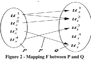
ii) Mapping Function
Mapping function denotes 𝑣(𝑢𝑠𝑖 )as the demand-traffic of 𝑢𝑖𝑠 , and v(𝑢𝑡𝑗) as the relay-traffic of𝑢𝑡𝑗 which measures the relay capability of an intermediate node.
Let P = 𝑢𝑠1, 𝑉(𝑢𝑠1)), … … ,𝑢𝑠𝑚,𝑉(𝑢𝑠𝑚)) be the state representation of m start nodes and Q = 𝑢𝑡1,𝑉(𝑢
𝑡
1) , … … . ,𝑢 𝑡 𝑛,𝑉(𝑢
𝑡
𝑛) be the state representation of n target nodes. So, the problem of transferring
the traffic from start nodes to their target nodes is converted into the link matching problem which can be. Formulated as Q=F (P) The mapping F= [𝑓𝑖𝑗 ]can transform P into Q Fig.4.2.2 below. This work is to find an optimal mapping where all the start nodes in P can find the target nodes in Q so that the total traffic can be transferred with minimum energy consumption.
Figure 2 - Mapping F between P and Q
Let D [ij] as the expected transmit count matrix among nodes in Us and Ut. Here, the expected transmit count between two nodes is 𝑢𝑠𝑖 and 𝑢𝑡𝑗is. 𝜂𝑖𝑗 1/(𝑑 𝑓𝑖𝑗 ×𝑑 𝑟𝑖𝑗 ) Let unit energy cost, denoted , equals to the
energy consumption of transmitting a bit. The entry 𝑓𝑖𝑗 of F denotes the traffic needed to be transported from 𝑢𝑠𝑖 to𝑢
𝑡
𝑖 . So, the optimization problem which minimizes the energy consumption can be expressed as
Minimize ( 𝑖∈𝑢𝑠 𝑖∈𝑢𝑡𝑓𝑖𝑗 𝑛𝑖𝑗 𝜀)
source initiates a route discovery process. It transmits multiple Route-Request messages to its neighboring nodes. The Route-request message includes different path ID’s to construct multiple node disjoint paths between the selected source and the destination, which should satisfy the following equation:
Next hop = 𝑎𝑟𝑔𝑚𝑖𝑛 𝑏∈𝑁𝑎 1− 𝑒𝑏 ,𝑟𝑒𝑠𝑖𝑑𝑢𝑎𝑙
𝑒𝑏 ,𝑖𝑛𝑖𝑡 [
𝛽 1− ∆𝑑+1
𝑑𝑎𝑦 ]
where Na represents the set of neighbors of node a, day represents the distance (hop count) between the node a and the sink node, dby represents the distance between node b and the sink node, ∆ d is the difference between day and dby, eb, init represents the initial battery level of node b, and β is the weight factor, and β > 1. As the sink receives the first Route-request message, it sets a timer to complete the route establishment process.
All the paths discovered after the timer expired are considered as low quality paths and the sink node discards the Route-request messages received from these paths.
After the route establishment process the sink node assigns data rates to the established paths through the following equation.
𝑟𝑗 = 𝑝𝑅
𝑗 𝑝𝑖,𝑗 =1,2, … … … … . .𝑁 𝑁
𝑖=1
here it is assumed that there are N paths between the source-sink nodes, rj is the assigned data rate to the jth path, R is the data rate requested by the application which should arrive at the sink node. pi and pj are the cost of ith and the jth path.
IV. ALGORITHMS USED IN PROPOSED SYSTEM
Duty cycling
Rendezvous Computation and Slot allocation
Co-operative Sharing Algorithm
4.1 Duty Cycling-
In this Algorithm, the lifetime of the node based on overall energy consumption is evaluated. The total energy consumption of the nodes consists of the energy consumed by listening, receiving, transmitting, sampling data and sleeping. Effect of duty cycle on the energy consumed by the nodes is also evaluated, based on the observations the optimum value of the duty cycle can be chosen. Duty Cycle provides a way to establish communications in the presence of sleeping nodes. Each sleeping node wakes up periodically to listen. If a node wants to establish communications, it starts sending out beacons polling a specific user. Within a bounded time, the polled node will wake up and receive the poll, after which the two nodes are able to communicate.
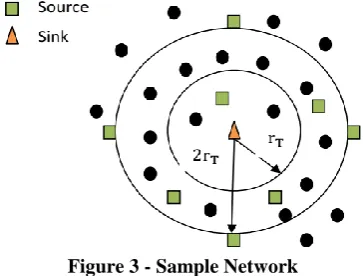
The traffic relayed at a node is related to its distance to the sink, the packet traffic generated by each source node, the number of source nodes in the network and the node density. The time required for a transmission and the energy efficiency of the network is closely related to the duty cycle values used. Higher values of duty cycle provide more nodes available for data routing and thereby energy consumption of the nodes increases.
Figure 3 - Sample Network
Nn nodes are considered in this ring. The average traffic that must be relayed by all of the nodes located in the nth ring per unit time, Γn, is the summation of the traffic generated by the source nodes in the nth ring and within the rings outside of the nth ring per unit time, i.e.,
𝑟𝑛 = 𝜆𝑔𝜌𝑠𝜋(𝑅2− [ 𝑛 −1 𝑟𝑇]2
Where, λF is the average traffic generation rate of the source nodes, ρ is the density of source node, R is the radius of the network area, rB is the transmission range. The traffic relayed at a node is depended on the node distance from the sink, the node density, the radius of the network area, and the transmission range. The average traffic rate of a node at distance r, λr, is
λ𝑟 =
λ𝑔𝜌𝑠𝜋 𝑅2− 𝑟 𝑇𝑟 −1 𝑟𝑇
2
𝜌𝑟𝜋 𝑟 𝑇𝑟 𝑟𝑇
2
− 𝑟 𝑇𝑟 −1 𝑟𝑇
2
The relay region (locations with geographic advancement to the sink) is divided into N priority regions, and each region is assigned a contention slot such that priority region i is assigned the ith slot in the contention window. To assign each priority region N CTS contention slots, such that priority region iis assigned the slots ((Ni-1) xNr, Ni, xNr-1). This reduces CTS collisions, as all nodes in priority region i can select one of the Nr CTS contention slots to send their CTS packet.
4.2 Duty Cycle for a Given Expected Traffic Rate-
The time required for a transmission and the energy efficiency of the network is closely related to the duty cycle values used. Higher duty cycle values provide more nodes available for data routing, such that the possibility to have no relay nodes is decreased and a lower latency is achieved, yet they consume more energy. In the duty cycle it minimizes the energy consumption for a given traffic rate.
Let N denote the average number of nodes within a node’s transmission range, d denote duty cycle, and λrdenote the average traffic rate of a node located at distance r to the sink node given in below equation. Assuming a Poisson or uniform packet generation rate, the average traffic rate of a node follows the Poisson distribution. The probability that a node detects no traffic can be calculated to be e-λrNTLwhere TL is its listen period at each cycle and λrNis the average packet arrival rate within its transmission range. The probability that a node detects any ongoing traffic is p0 = 1 - e-λrNTL. If ξ is the ratio of the relay region (i.e., the region in which nodes make forward progress to the sink) to the transmission area, p0ξ is the probability of a node detecting ongoing traffic and residing in the relay region of that traffic.
𝑖 1−𝑝1 𝑖 𝛼
𝑖=1 𝑝1=
1−𝑝1
𝑝1 = 𝑒
𝜀𝑑 𝑁−1 −1
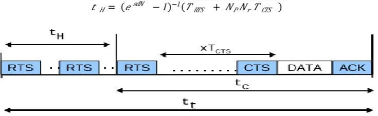
where p1 = 1-e-ξdN is the probability that at least one node replies to the RTS packet, since the number of nodes residing in an area can be approximated by Poisson distribution for uniformly random deployment. For each retransmission, the node sends out an RTS packet and waits for Np × Nr CTS slot durations. The expected time needed before the first successful RTS/CTS handshake, tH, is then
𝑡𝐻= 𝑒𝜀𝑑𝑁 −1 −1 𝑇
𝑅𝑇𝑆 + 𝑁𝑃𝑁𝑟𝑇𝐶𝑇𝑆
Figure 4 - Duty Cycle for a Given Expected Traffic Rate
4.3 Packet Exchange Duration-
Where TRT S and TCT S are the transmission delays for RTS and CTS packets, respectively. As shown in Figure 4. above, the expected total time for a complete RTS, CTS, DATA and ACK packet communication is
𝑡 𝐶 = 𝑇𝑅𝑇𝑆 +𝑥 𝑇𝐶𝑇𝑆 + 𝑇𝐷𝐴𝑇𝐴 + 𝑇𝐴𝐶𝐾
wherex represents the number of CTS contention slots up to and including the first successful CTS packet, TDAT A and TACK are the required times for DATA and ACK packets, respectively. The formula for x can be calculated from a standard CSMA model, and we omit it here for the sake of brevity. Therefore, the expected total time for a node to transmit a packet, including all the failed RTS packets and the successful data exchange is tt= tH+ tC.
The expected time for a node to receive an RTS packet during a listening period is T2 L. An approximation for the probability that a node wins the contention and is selected as the relay node is given as 1 - e-ξdNξdN. Then, the average active time of a node that receives traffic and that resides in the relay region of the sender node is
𝑡 1=
𝑇𝐿
2 +
1−𝑒−𝜀𝑑𝑁
𝜀𝑑𝑁 𝑡 𝑐 + 1−
1−𝑒−𝜀𝑑𝑁
𝜀𝑑𝑁
𝑇𝐿
2
Finally, the expected time a node is awake during one listen period is tl= (1-p0ξ)TL+p0ξt1, where (1-p0ξ) represents the probability that either a node hears no traffic or hears some traffic but is not in the relay region, in which case the node is awake for TL time.
4.4 Duty Cycle Assignment Method-
However, RTS packets can be used to observe the traffic load. The number of retransmitted RTS packets increases either when a node’s duty cycle is too low and no relay candidates can be found, or when the traffic load is too high and the high contention of nodes causes collisions of the RTS packets from different transmitters. For either case, increasing the duty cycle would increase the probability of successful communication. To introduce a piggyback flag to the original packet header of the RTS packet to indicate whether this packet is being retransmitted or not. A counter is also set in every node to record the numbers of the initial and retransmitted RTS packets. If the total number of the received retransmitted RTS packets in the current cycle outweighs the total number of the received initial RTS packets, it indicates severe contention in the neighborhood, and the duty cycle of the node is increased to mitigate the traffic load.
Otherwise, the duty cycle is decreased every cycle down to a minimum of 1% to minimize the energy consumption. This method is called Traffic Adaptive Distance-based Duty Cycle Assignment. This is expected to improve the latency performance, since it takes into account not only the distance-based duty cycle assignment, but also the spatiotemporal traffic information in a particular network deployment.
4.5 Utilization Based Tuning of Duty Cycle-
Every node in a sensor network have their own different traffic loads according to what tasks they take and where the locations they are. To reflect the different traffic loads, to adopt the utilization of each node as the evaluation metric. Upon synchronization time, the node calculates its utilization after the last synchronization time. It adjusts its duty cycle according to the calculated utilization, and then sends the new schedule to its neighbors via broadcasting.
The node first calculates the utilization U as Trx+Ttx+Trx+Ttx+Tidle,where the Trxstands for total receiving time, Ttxstands for total transmitting time, and Tidlestands for total idle listening time during this synchronization interval. Both of the total receiving and total transmitting time are the time that a node staying in receiving and transmitting states respectively. The total idle listening time is the time that a node staying in listening state without involving in any transmission process. If the utilization U of a node is high, the traffic load is too heavy for the current listening schedule to afford. Therefore, it should increase the duty cycle to fit the requirement of such heavy traffic load. In the proposed scheme, It define Uhighas the threshold of high traffic load. Once upon the node is considered as high utilization, the duty cycle will increased by n%. Larger n results in faster adaption of traffic loads, but smaller n avoids the excessive response and helps finding out best schedule under different traffic loads. Besides, to provide the guarantee of maximum energy consumption, our proposed algorithm also sets the upper limit of duty cycle, DCmax. A node stops increasing its duty cycle if the current duty cycle reaches DCmax. Similarly, a node will decrease its duty cycle as the utilization U is smaller than Ulow, the threshold of low traffic, and stop decreasing its duty cycle if reach the defined lower bound of duty cycle, DCmin.
4.6 Selective Sleeping after Transmission-
A node goes to sleep due to scheduled sleep time arrived or after reception of control packets such as RTS and CTS not destined to itself. However, the MAC protocol can get extra energy saving from sleeping after transmission.
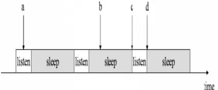
As shown in Figure 5. above, a transmission may end at scheduled listen time like”a”, or scheduled sleep time like”b”. If a transmission ends at scheduled sleep time b, the node will keep listening until the next scheduled sleep time d, so that between b and the next scheduled listen time c, the energy is wasted. To avoid the above energy wastage, it shows that a node should go to sleep “selectively”. When transmission is completed, a node checks if it is at scheduled sleep time. It goes to sleep if it’s at scheduled sleep time. The sleep will not result in additional delay since the node is considered as sleep on its neighboring nodes, and no node will send packet for the node.
Assuming packet transmission will end with equal probability within a frame at the receiver, let Tframedenote the complete cycle time of listen and sleep schedule. The average sleep time due to selective sleeping is
𝑇𝑓𝑟𝑎𝑚𝑒 2
The above is similar to the calculation of sleep delay. As described in SMAC, the Tframeis
𝑇𝑓𝑟𝑎𝑚𝑒 =
𝑇𝑙𝑖𝑠𝑡𝑒𝑛 𝑑𝑢𝑡𝑦𝑐𝑦𝑐𝑙𝑒
And Tlistenis a fixed length listen period within a frame. It shows that selective sleeping can achieve energy saving per transmission as:
𝑇𝑙𝑖𝑠𝑡𝑒𝑛
2 ×𝑑𝑢𝑡𝑦𝑐𝑦𝑐𝑙𝑒 × (𝑃𝑖𝑑𝑙𝑒 −𝑃𝑠𝑙𝑒𝑒𝑝 )
Where Pidleand Psleepstand for power consumption of idle and sleep state, respectively. According to the above formula, it shows that the energy saving from selective sleeping can be more significant when it tuned down the duty cycle.
V. SIMULATION RESULTS
Simulation is the impersonation of the activity of a certifiable procedure or framework after some time. The demonstration of reenacting something initially necessitates that a model be created; this model speaks to the key qualities, practices and elements of the chose physical or conceptual framework or process. The model speaks to the framework itself, though the simulation speaks to the task of the framework after some time. In simulation, by making a numerical model of a framework or process, more often than not on a PC, and we investigate the conduct of the model by running a simulation. A simulation comprises of numerous regularly a great many preliminaries. Every preliminary is an examination where clients supply numerical qualities for input factors, assess the model to process numerical qualities for results of intrigue, and gather these qualities for later investigation.
The part of simulation investigation is to abridge and examine the outcomes, in a way that will yield most extreme knowledge and help with basic leadership. It is exceptionally helpful to make outlines and envision the outcomes, for example, recurrence graphs and combined recurrence diagrams.
The Simulation consequences of this work are examined and abridged as takes after
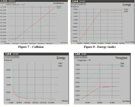
Figure 7 – Collision Figure 8 - Energy (node)
Figure 9 - Energy (link) Figure 10 - Throughput
Table - 1 Simulation Parameters
PARAMETERS CMAC RAPS
BANDWIDTH (Hz/s) 45 102
COLLISION 249 200
ENERGY (J/p) 1.5 0.1
THROUHPUT (p/s) 600 1500
ENERGY (J/P) 0.2 0.4
Table - 2 Simulation Parameters
PARAMETER VALUE
NETWORK REGION 1400×1400
NO. OF NODES 100
INITIAL ENERGY 20J
RP DSR
SIMULATION TIME 30S
NO.OF PACKETS 1500
FREQUENCY 2.4GHz
CHANNEL WIRELESS
VI. CONCLUSION
In this paper, a novel coordination-based MAC protocol for a wireless ad hoc network has been proposed. In the proposed MAC scheme, the network zone is apportioned into cells and a facilitator node intermittently plans all transmissions/gatherings for nodes inside its cell.For each planned transmission/gathering, the channel in both time and space do-mains are held to evade transmission collisions. Adjacent organizers trade scheduling data to augment spatial spectrum reuse while maintaining a strategic distance from transmission collision. A source node fights just once to transmit a cluster of packets. After that it can ask for transmission by incorporating the data in the header of one data packet. In addition, occasional scheduling of transmission time spaces for data packets enables a node to put its radio interface into the rest mode when not transmitting/accepting a packet keeping in mind the end goal to lessen vitality utilization.
Therefore by looking at the execution of the proposed scheme with the IEEE 802.11 DCF scheme without control sparing and in control sparing mode, whose carrier sensing range and ATIM measure are powerfully adjusted to give most astounding throughput. The execution measures incorporate total throughput, normal vitality utilization per packet and packet collision rate. Reproduction results demonstrate that the proposed scheme achievers generously higher throughput, altogether lessens vitality utilization, and has a considerably littler packet collision rate in correlation with the current protocols. Disseminating organizers in the network territory based on network condition examination and adjusting transmission control level of network joins are further research headings to improve network limit and lessen vitality utilization.
REFERENCES
[1] “Cisco visual networking index: Global mobile data traffic forecast update, 2013-2018,” White Paper, Cisco, Feb. 2014.
[2] K. RahimiMalekshan, W. Zhuang, and Y. Lostanlen, “An energy efficient MAC protocol for fully connected wireless ad hoc networks,”IEEE Trans. Wireless Communications, vol. 13, no. 10, pp. 5729– 5740,Oct. 2014.
[3] S. Ramanathan, “A unified framework and algorithm for (T/F/C) DMAchannel assignment in wireless networks,” inProc. IEEE INFOCOM’97, Apr. 1997.
[4] A. Ephremides and T. Truong, “Scheduling broadcasts in multihop radio networks,”IEEE Trans. Communications, vol. 38, no. 4, pp. 456–460, Apr. 1990.
[5] J. Zhu, X. Guo, L. Yang, and W. Conner, “Leveraging spatial reuse in802.11 mesh networks with enhanced physical carrier sensing,” inProc.IEEE ICC’04, June 2004.
[6] IEEE 802.11 WG, Part 11: Wireless LAN Medium Access Control (MAC) and Physical Layer (PHY) Specification, Standard, Aug. 1999.
[7] Z. Abichar and J. Chang, “Group-based medium access control for IEEE802.11n wireless LANs,”
[8] IEEE Tran. Mobile Computing,, vol. 12, no. 2,pp. 304–317, July 2013.
[9] W. Ye, J. Heidemann, and D. Estrin, “Medium access control with coordinated adaptive sleeping for wireless sensor networks,”IEEE/ACMTran. Networking, vol. 12, no. 3, pp. 493– 506, June 2004.
[10] T. van Dam and K. Langendoen, “An adaptive energy-efficient MAC protocol for wireless sensor networks,” inProc. ACM SenSys’03, Nov.2003.