Performance Analyses of Recurrent Neural Network Models Exploited for Online Time-Varying Nonlinear Optimization

Performance Analyses of Recurrent Neural Network

Models Exploited for Online Time-Varying Nonlinear

Optimization

Mei Liu1, Bolin Liao2,3, Lei Ding2,3, and Lin Xiao2,3

1_{College of Physics, Mechanical and Electrical Engineering, Jishou University, Jishou, 416000,}

Hunan, China [email protected]

2

College of Information Science and Engineering, Jishou University, Jishou, 416000, Hunan, China

3_{The Collaborative Innovation Center of Manganese-Zinc-Vanadium Industrial Technology (the}

2011 Plan of Hunan Province), Jishou, 416000, Hunan, China [email protected], [email protected], [email protected]

Abstract. In this paper, a special recurrent neural network (RNN), i.e., the Zhang neural network (ZNN), is presented and investigated for online time-varying non-linear optimization (OTVNO). Compared with the research work done previously by others, this paper analyzes continuous-time and discrete-time ZNN models the-oretically via rigorous proof. Theoretical results show that the residual errors of the continuous-time ZNN model possesses a global exponential convergence prop-erty and that the maximal steady-state residual errors of any method designed in-trinsically for solving the static optimization problem and employed for the online solution of OTVNO isO(τ), whereτ denotes the sampling gap. In the presence of noises, the residual errors of the continuous-time ZNN model can be arbitrarily small for constant noises and random noises. Moreover, an optimal sampling gap formula is proposed for discrete-time ZNN model in the noisy environments. Fi-nally, computer-simulation results further substantiate the performance analyses of ZNN models exploited for online time-varying nonlinear optimization.

Keywords:performance analysis, Zhang neural network (ZNN), online time-varying nonlinear optimization (OTVNO), Newton conjugate gradient model.

1.

Introduction

The recurrent neural network (RNN) has received considerable investigation in many scientific and engineering fields, which has several potential advantages in real-time ap-plications (e.g., parallel processing, distributed storage, self adaptation) [4, 10–17]. There-fore, the RNN is generally taken into account as one of the powerful parallel-computational schemes for online solution of various challenging problems [13, 15, 17]. As a novel type of RNN specifically designed for solving time-varying problems, Zhang neural network (ZNN) is able to perfectly track time-varying solution by exploiting the time derivative of time-varying parameters [4, 11, 17–19]. Different ZNN models have been proposed in [4] for solving online time-varying nonlinear optimization (OTVNO) problem in the presence of zero noise.

In implementations of an RNN model, we usually assume that it is free of all kinds of noises or external errors [9]. However, there always exist some realization errors in hard-ware implementations or disturbances in applications of RNN, which can be deemed as constant noises. Moreover, the environmental interference as well as other external errors can be viewed as the random noises. Sometimes these noises have significant impacts on the accuracy of the RNN for solving time-varying problems, and in some cases, they may cause failure of the solving task. Therefore, it is worth investigating the performance of ZNN models from the control perspective for solving time-varying nonlinear optimization problem with rigorous proof.

The rest of this paper is organized as follows. Section 2 introduces the problem for-mulation and presents the ZNN models for online solution of time-varying optimization problem. In addition, Section 3 provides the related work done by others and the cor-responding analysis. The convergence and robustness analyses of the ZNN models are presented in Section 4. In Section 5, illustrative simulative results are shown to verify the convergence and robustness of the ZNN model for solving time-varying nonlinear opti-mization problem, which further substantiate the theoretical analysis. Finally, conclusions are drawn in Section 6. Before ending this introductory section, the main contributions of the paper are pointed out below.

– The online time-varying nonlinear optimization problem is investigated. Its solution is obtained using the continuous-time and discrete-time ZNN models with satisfactory performance.

– Theoretical analyses and results for continuous-time ZNN model are presented, which guarantee that its residual error possesses a global exponential convergence property. Moreover, in the presence of noises, its residual error can be arbitrarily small for constant noises and random noises.

– Theoretical analyses and results also show that the maximal steady-state residual er-rors of any method designed intrinsically for solving the static optimization problem and employed for the online solution of OTVNO isO(τ). In addition, the optimal sampling gap formula for discrete-time ZNN model in noisy environments is pro-posed.

2.

Problem formulation and ZNN solution

As a basis for further discussion, the problem formulation for online time-varying opti-mization and continuous-time and discrete-time ZNN models are presented in this section.

2.1. Problem formulation

Let us consider the following time-varying optimization problem in a continuous form, which is the same task problem presented in [4]:

min

x(t)∈Rn

f x(t), t

∈R, t∈[0,+∞), (1)

where the second-order differentiablef(·,·) : Rn ×[0,+∞) → Rdenotes a nonlin-ear mapping function. In addition, the gradient of (1) can be formulated asg(x(t), t) =

∂f(x(t), t)/∂x(t).

2.2. ZNN Solution

Defining the error functione(t) =g(x(t), t), we show how to design the corresponding continuous-time ZNN model via the ZNN design formula. Let us define the following evolution fore(t):

˙

e(t) =−γe(t), (2)

whereγ >0is a scaling factor. ZNN design formula (2) indicates thate˙(t)is evaluated as the negative direction ofe(t)such thate(t)converges to zero, which means thatx(t) converges to the zero point x∗(t)ofe(t). By expanding the ZNN design formula, the following differential equation of a ZNN model is obtained:

H(x(t), t) ˙x(t) =−γg(x(t), t)−g′t(x(t), t), (3)

where Hessian matrix H(x(t), t) and time-derivative vectorg′

t(x(t), t) are defined re-spectively as [4]:

H(x(t), t) = ∂g(x(t), t)

∂xT_(t) =

∂2_{f(x(t), t)} ∂x(t)∂xT_(t)∈R

n×n_,

g′

t(x(t), t) =

∂g(x(t), t)

∂t =

∂2_{f(x(t), t)} ∂x(t)∂t ∈R

n_,

with superscriptT denoting the transpose of a vector or matrix argument. For the inter-esting nonsingular situation ofH(x(t), t)that we consider in this paper, (3) is rewritten as

˙

x(t) =−H−1_{(x(t), t)γg(x(t), t) +}∂g(x(t), t) ∂t

(4)

+

+ +

+

−

R

e(t)

−e(t)

0 g(x(t), t)

reference

output

ZNN model RTVNO problem

x(t) ˙

x(t) γ

−g′

t(x(t), t)

I−H(x(t), t) dx_d(t)t

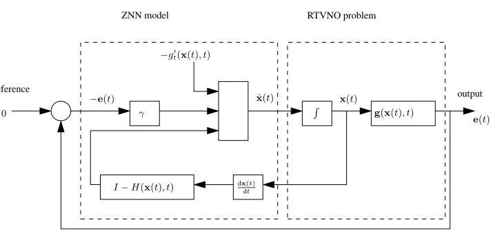
Fig. 1.Realization of continuous-time ZNN model (4) for solving OTVNO problem (1) represented as a feedback control system.

that, to focus on the performance analyses of ZNN models, we consider the situation that H(x(t), t)is positive definite in this paper.

In terms of OTVNO problem (1), continuous-time ZNN model (4) is an equivalent expansion of ZNN design formula (2). For a better understanding of ZNN design formula (2) as well as continuous-time ZNN model (4), the role of each term in ZNN design for-mula (2) can be interpreted from the viewpoint of control with its realization represented as a control system shown in Fig. 1. From the figure, we can find that continuous-time ZNN model (4) can be deemed as a generalized proportional-derivative controller with the control input for the derivative part beingx˙(t)and that for the proportional part being

e(t). For such a control system, it will be proven in the ensuing Theorem 2 thate(t) glob-ally and exponentiglob-ally converges to zero, which means that the presented continuous-time ZNN model (4) possesses the property of globally exponential stability.

The corresponding discrete-time ZNN model [4] based on Euler forward difference formula can be directly given as

xk+1 =xk−H−1(xk, tk) (hg(xk, tk) +τ g′t(xk, tk)), (5) where step-sizeh=τ γ >0, withτdenoting the sampling gap.

3.

Related work

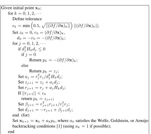
Table 1.Pseudocode of Newton-CG method Given initial pointx0;

fork= 0,1,2,· · ·

Define tolerance ǫk=min

0.5,p

||(∂f /∂x)k||

||(∂f /∂x)k||;

Setz0= 0,r0= (∂f /∂x)k,

d0=−r0=−(∂f /∂x)k;

forj= 0,1,2,· · ·

ifdT

jHkdj≤0

ifj= 0

Returnpk=−(∂f /∂x)k;

else

Returnpk=zj;

Setaj=rTjrj/dTjHkdj;

Setzj+1=zj+ajdj;

Setrj+1=rj+ajHkdj;

If||rj+1||< ǫk

returnpk=zj+1;

Setβj+1=rj+1T rj+1/rTjrj;

Setdj+1=−rj+1+βj+1dj;

end (for)

Setxk+1=xk+akpk, whereaksatisfies the Wolfe, Goldstein, or Armijo

backtracking conditions [1] (usingak= 1if possible);

end

maximal steady-state residual error of Newton-CG method for solving OTVNO problem (1) isO(τ).

THEOREM1.Suppose that the Newton-CG method converges to the optimal solution to a static optimization problem within computational timeτ. If the Newton-CG method is employed for OTVNO (1), then the maximal steady-state residual error_kg(xk+1, tk+1)k2 of Newton-CG method isO(τ).

Proof. As assumed, the time derivative of xi(t)exists, i.e., dxi(tk)/dt = pi at time instanttk withpi being a constant. It can be readily derived thatlimτ→0∆xi(tk)/τ = dxi(tk)/dt=piand∆xi(tk)≈piτ. Therefore,∆xi(tk)changes in anO(τ)pattern, i.e., ∆xi(tk) =O(τ). Note that, at computational time interval[kτ,(k+ 1)τ), the Newton-CG method converges to the optimal solutionx∗

i(tk)to the time-varying optimization problem at time instant tk andx∗i(tk+1) = xi∗(tk) + ∆xi(tk). Thus, at time instant tk+1, the difference between the solution generated by the Newton-CG method and the optimal solution is∆x(tk), i.e.,x∗(tk+1) =x∗(tk) +O(τ) =x(tk+1) +O(τ), where

theorem, we obtain

g(xk+1, tk+1) =g x∗k+1+O(τ), tk+1

=g(x∗_k+1, tk+1) +H(xk+1∗ , tk+1)O(τ) +O(τ2) =H(x∗_k+1, tk+1)O(τ) +O(τ2)

=H(x∗_k+1, tk+1)O(τ).

Consequently, we further have

kg(xk+1, tk+1)k2=kH(xk+1∗ , tk+1)O(τ)k2=O(τ).

The proof is thus completed.

As proven in [4], the maximal steady-state residual error of discrete-time ZNN model (5) possesses anO(τ2_{)pattern. Actually, it can be generalized from Theorem 1 that the} maximal steady-state residual errors of any method designed intrinsically for solving the static optimization problem and employed for the online solution of OTVNO isO(τ). The above analysis further demonstrates the superiority of discrete-time ZNN model (5) for OTVNO solving (compared with the conventional methods).

4.

Theoretical analyses

In this section, we prove thate(t)of continuous-time ZNN model (4) globally and expo-nentially converges to zero. In addition, in the presence of noises, continuous-time ZNN model (4) is proven to have a satisfactory robust performance. Moreover, an optimal sam-pling gap formula is proposed for discrete-time ZNN model in the noisy environments.

THEOREM2.Continuous-time ZNN model (4), starting with randomly generated ini-tial statex(0)∈Rn, globally and exponentially converges to the theoretical solution to OTVNO (1).

Proof. ZNN design formula (2) is a compact vector-form equations with itsith element beinge˙i(t) =−γei(t). By defining the Lyapunov function candidatevi(t) =e2i(t)with

˙

vi(t) = −2γe2i(t), it can be readily generalized that continuous-time ZNN model (4) globally converges to theoretical solutionx∗_{(t)to OTVNO (1).}

In addition, from ZNN design formula (2), one can readily conclude that e(t) =

e(0) exp(−γt)withe(0)denoting the initial error of continuous-time ZNN model (4). Therefore, it can be readily generalized that continuous-time ZNN model (4) exponen-tially converges to theoretical solutionx∗(t)to OTVNO (1).

The proof is thus completed.

To investigate the performance of continuous-time ZNN model (4) in the presence of noises, two theorems on the constant noise and the random noise are presented as follows. THEOREM3.Consider that continuous-time ZNN model (4) is polluted with con-stant noise η(t) = ¯η ∈ Rn. Continuous-time ZNN model (4) converges towards the-oretical solution x∗_{(t)to OTVNO (1) with the upper bound of the steady-state} resid-ual errorlimt→∞ke(t)k2 being kη¯k2/γ. Furthermore, the steady-state residual error limt→∞ke(t)k2decreases to zero asγtends to positive infinity.

Proof. Using Laplace transform to the ith subsystem of the noise-polluted continuous-time ZNN model (4) leads to

sei(s)−ei(0) =−γei(s) +ηi(s), (6)

i.e.,

ei(s) = ei(0) +ηi(s)

s+γ , (7)

with the transfer function being1/(s+γ), where the pole is s = −γ. Forγ > 0, it can be readily concluded that this pole locates on the left half-plane, which implies that this system is stable and that the final value theorem applies. Notice thatηi(s) = ¯ηi/sas ηi(t) = ¯ηi amounts to a step signal for constant vectorη¯. Using the final value theorem to (7), we have

lim

t→∞ei(t) = lims→0sei(s) = lims→0

s(ei(0) + ¯ηi/s) s+γ =

¯

ηi γ.

Therefore, it can be concluded thatlimt→∞ke(t)k2=kη¯k2/γ. Furthermore, the steady-state residual errorlimt→∞ke(t)k2decreases to zero asγtends to positive infinity. The proof is thus completed.

Note that the nonlinear time-varying noise can be deemed as a random noise in the time-varying nonlinear optimization problem solving process, and we have the follow-ing theorem for the performance of continuous-time ZNN model (4) in the presence of unknown random noise.

THEOREM4.Consider that continuous-time ZNN model (4) is polluted with bounded random noiseη(t) =σ(t)∈Rn. Continuous-time ZNN model (4) converges towards the-oretical solutionx∗_{(t)to OTVNO (1) with the upper bound of the steady-state residual} errorlimt→∞ke(t)k2 being (ξ√n)/γ withξ = max1≤i≤n{max0≤τ≤t|σi(τ)|}. Fur-thermore, the steady-state residual errorlimt→∞ke(t)k2decreases to zero asγtends to positive infinity.

Proof. Rewrite random-noise-polluted continuous-time ZNN model (4) as ˙

e(t) =−γe(t) +σ(t),

of which theith (∀i∈1,2,· · ·, n) subsystem can be written as ˙

ei(t) =−γei(t) +σi(t). (8)

ei(t) =ei(0) exp(−γt) +

Z t

0

exp(−γ(t−τ))σi(τ)dτ.

From the triangle inequality, we have

|ei(t)| ≤ |ei(0) exp(−γt)|+

Z t

0 |

exp(−γ(t−τ))||σi(τ)|dτ.

We further have

|ei(t)| ≤ |ei(0) exp(−γt)|+ 1

γ0max≤τ≤t|σi(τ)| Finally, we have

lim

t→∞supke(t)k2≤

ξ√n γ ,

withξ= max1≤i≤n{max0≤τ≤t|σi(τ)|}. The proof is thus completed.

It is worth noting that, for discrete-time ZNN model (5), the sampling gapτ, the noise corruption, the round-off errors as well as the truncation errors have influences on the total error, and thus a smaller sampling gapτdoes not necessarily generate a smaller total error. Therefore, it is worth investigating the performance of discrete-time ZNN model (5) in the presence of noise and finding the optimal sampling gap.

THEOREM5.The optimal sampling gap of discrete-time ZNN model (5) isτoptimal=

2((ε+σ)/M)1/2_{, whereεdenotes the maximum absolute value of round-off errors ofx} k andxk+1in the numerical computations,σdenotes the upper bound of the noise, andM denotes the maximum absolute value ofx¨k+cwithclying between0and1.

Proof. Based on the Taylor expansion, we have the following rule:

xk+1=x(kτ+τ) =xk+τx˙k− τ2

2!x¨k+c, (9)

whereclies between0and1. Then, withM denoting the maximum absolute value of ¨

xk+c, we have the following Euler forward difference formula with truncation error:

˙

xk =

xk+1−xk

τ +

τ

2M, (10)

The round-off errors and the noises in the numerical computations can be simplified as following equations:

xk+1 =yk+1+εk+1+ξk+1,

xk =yk+εk+ξk,

wherexk+1andx0are approximated by numerical valuesyk+1andyk, respectively. In addition,εk+1 andεk are the corresponding round-off errors. Besides,ξk+1 andξ0are the corresponding noises with the upper bound beingσ.

According to (10), we can obtain

˙

xk=

yk+1−yk

0

2

4

6

8

10

0

5

10

15

20

25

0

0.5

1

1.5

2

0

2

4

ke(t)k2

t(s)

γ= 10 γ= 1

Fig. 2.Residual errors of continuous-time ZNN model (4) for solving OTVNO (13) with initial state

x(0) = [0,4,−8,−6]T.

in which

E(x, τ) = εk+1+ξk+1−εk−ξk

τ +

τ M

2 .

Evidently, the total error termE(x, τ)contains two parts, i.e., a part due to round-off errors as well as the noise corruption, and a part due to truncation errors.

Considering thatεdenotes the maximum absolute value of round-off errors ofxkand

xk+1and that the upper bound value ofξkandξk+1isσ, we have

|E(x, τ)| ≤ 2(ε_τ+σ)+τ M

2 . (11)

Thus, the value ofτthat minimizes the right-hand side of formula (11) is

τoptimal= 2

_ε+σ

M

1/2

. (12)

The proof is thus completed.

5.

Illustrative examples

0

2

4

6

8

10

0

5

10

15

20

25

9

9.5

10

0

0.5

1

1.5

ke(t)k2

t(s)

γ= 10 γ= 1

Fig. 3.Residual errors of continuous-time ZNN model (4) for solving OTVNO (13) with initial state

x(0) = [0,4,−8,−6]Tand constant noise[1,1,1,1]T.

In this section, computer-simulation results and observations are provided to verify the characteristics of these models.

5.1. Continuous-time ZNN model

Example 1.For illustration and comparison, let us consider the following time-varying nonlinear optimization problem, which is the same problem as in [4]:

min

x(t)∈R4

f(x(t), t) = (x1(t) +t)2+ (x2(t) +t)2+ (x3(t)−exp(−t))2

+ 0.1(t−1)x3(t)x4(t)−(x1(t) + ln(0.1t+ 1))(x2(t) + sin(t)) + (x1(t) + sin(t))x3(t) + (x4(t) + exp(−t))2. (13)

0

2

4

6

8

10

0

5

10

15

20

25

8

8.5

9

0

0.2

0.4

ke(t)k2

t(s)

γ= 10 γ= 1

Fig. 4.Residual errors of continuous-time ZNN model (4) for solving OTVNO (13) with initial state

x(0) = [0,4,−8,−6]Tand constant noiseσ(t)∈[−0.5,0.5]4×1.

for a large constant bias noise. Therefore, it is worth investigating the performance of continuous-time ZNN model (4) in the presence of constant noise.

As visualized in Fig. 3(a), the residual error of continuous-time ZNN model (4) with γ = 1rapidly converges towards zero and remains stable around1.7. In addition, the residual error of continuous-time ZNN model (4) with γ = 10also rapidly converges towards zero and remains stable at the order of10−1_{. In summary, these results verify} Theorem3.

In the solving process of OTVNO problem (1), noise is an external error or undesired disturbance, which misdirects the conventional model to evolve along a wrong direction. Numerous methods have been presented and investigated for denoising, such as Wiener filtering and Kalman filtering as well as their extensions. However, by considering the facts that many types of noises may not satisfy the requirements of the denoising method, and that any preprocessing for noise reduction may consume extra time, possibly vio-lating the requirement of real-time computation, conventional denoising methods may be not available for OTVNO problem (1). In addition, the nonlinear time-varying noises can be deemed as random noises. Therefore, it is worth investigating the performance of continuous-time ZNN model (4) in the presence of random noises. The corresponding simulation results are illustrated in Fig. 4.

10

10

10

10

10

10

10

10

10

10

10

10

10

10

ke(t)k2

σ τ= 0.01

τ= 0.1

Fig. 5.Means of residual errors of discrete-time ZNN model (5) withh= 1in noisy environments for 10 trials.

addition, the residual error of continuous-time ZNN model (4) withγ = 10also rapidly converges towards zero and remains stable at the order of10−2_.

In summary, the above simulation results, i.e., Figs. 2 through 4, have verified the correctness of the presented Theorem 2 through Theorem 4.

5.2. Discrete-time ZNN model

It is worth investigating the performance of discrete-time ZNN model (5) in noisy envi-ronments.

Example 2.Consider the following time-varying nonlinear optimization problem: min

x(t)∈R2f(x(t), t) =x 3

1(t)−sin(t)x21(t) + sin 2_(t)x

1(t) +x32(t)

−cos(t)x22(t) + cos2(t)x2(t). (14)

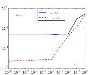
environment is of order10−16_(i.e.,2−52_{). Thus, we haveM = 1andε= 2.2×10}−16_. The values ofσthat do not influence the performance of discrete-time ZNN model (5) are 2.5×10−3_and2.5×10−5_{corresponding to using sampling gapτ= 0.1and0.01,} respec-tively. Means of residual errors of discrete-time ZNN model (5) with zero-mean noises for 10 trials are shown in Fig. 5. As seen from the figure, starting with the randomly-generated initial state, the performance of discrete-time ZNN model (5) does not reduce forσ < 10−3_{withτ = 0.1, and forσ < 10}−5_{withτ = 0.01. In addition, for the} up-per boundσ > (τ2_{M −4ε)/4, it can be observed from the figure that the noises have} remarkable impacts on the performance of discrete-time ZNN model (5), which means that some noise reduction technologies can be considered for better performance. For ex-ample, as often done in real-world implementation of the proportional-integral-derivative controller, it is preferable to pass the signals through the low-pass filter before they go to discrete-time ZNN model (5) to reduce the sensitivity of discrete-time ZNN model (5) to noise.

6.

Conclusions

In this paper, the Zhang neural network (ZNN) has been presented and investigated for online time-varying nonlinear optimization (OTVNO). Compared with the research work done previously by others, this paper has analyzed continuous-time and discrete-time ZNN models theoretically via rigorous proof. Theoretical results have shown that the maximal steady-state residual errors of the continuous-time ZNN model possesses a global exponential convergence property and that the maximal steady-state residual errors of any method designed intrinsically for solving the static optimization problem and employed for the online solution of OTVNO isO(τ). Moreover, in the presence of noises, the resid-ual errors of the continuous-time ZNN model can be arbitrarily small for constant noises and random noises. Finally, computer-simulation results have further substantiated the performance analyses of ZNN models exploited for online time-varying nonlinear opti-mization.

Acknowledgements.This work was supported in part by the National Natural Science Founda-tion of China under Grants 61563017, 61503152 and 61363073, in part by the Scientific Research Fund of Hunan Provincial Education Department under Grant 13A075, and in part by the Doctoral Scientific Research Foundation of Jishou University under Grant jsdxxcfxbskyxm06.

References

1. Bhaya, A., Kaszkurewicz, E.: Control Perspectives on Numerical Algorithms and Matrix Prob-lems. SIAM, Philadelphia, PA (2006)

2. Zhang, F., Han, Z., Ge. H., Zhu, Y.: Optimization design of traffic flow under security based on cellular automata model. Computer Science and Information Systems 12(2), 427–443 (2015) 3. Li, S., Li, Y., Wang, Z.: A class of finite-time dual neural networks for solving quadratic

programming problems and its k-winners-take-all application. Neural Networks 39(1), 27–39 (2013)

5. Guo, D., Zhang, Y.: Simulation and experimental verification of weighted velocity and ac-celeration minimization for robotic redundancy resolution. IEEE Transactions on Automation Science and Engineering 11(4), 1203–1217 (2015)

6. Jin, L., Zhang, Y.: G2-type SRMPC scheme for synchronous manipulation of two redundant robot arms. IEEE Transactions on Cybernetics 45(2), 153–164 (2015)

7. Luo, Q., Ma, M., Zhou, Y.: A novel animal migration algorithm for global numerical optimiza-tion. Computer Science and Information Systems 13(1), 259–285 (2016)

8. Liao, B., Zhang, Y., Jin, L.: TaylorO(h3)discretization of ZNN models for dynamic equality-constrained quadratic programming with application to manipulators. IEEE Transactions on Neural Networks and Learning Systems 27(2), 225–237 (2016)

9. Jin, L., Zhang, Y., Li, S.: Integration-enhanced Zhang neural network for real-time varying ma-trix inversion in the presence of various kinds of noises. IEEE Transactions on Neural Networks and Learning Systems. In Press with DOI being 10.1109/TNNLS.2015.2497715.

10. Guo, D., Zhang, Y.: Zhang neural network for online solution of time-varying linear matrix in-equality aided with an in-equality conversion. IEEE Transactions on Neural Networks and Learn-ing Systems 25(2), 370–382 (2014)

11. Zhang, Y., Yi, C.: Zhang Neural Networks and Neural-Dynamic Method. Nova Science Pub-lishers, New York (2011)

12. Jin, L., Zhang, Y.: Discrete-time Zhang neural network ofO(τ3_{)pattern for time-varying}

ma-trix pseudoinversion with application to manipulator motion generation. Neurocomputing 142, 165–173 (2014)

13. Li, S., Liu, B., Li, Y.: Selective positive-negative feedback produces the winner-take-all com-petition in recurrent neural networks. IEEE Transactions on Neural Networks and Learning Systems 26(2), 301–309 (2013)

14. Jin, L., Zhang, Y.: Continuous and discrete Zhang dynamics for real-time varying nonlinear optimization. Numerical Algorithms. In Press with DOI being 10.1007/s11075-015-0088-1. 15. Jin, L., Zhang, Y., Li, S., Zhang, Y.: Noise-tolerant ZNN models for solving time-varying

zero-finding problems: A control-theoretic approach. IEEE Transactions on Automatic Control. In Press with DOI being 10.1109/TAC.2016.2566880.

16. Li, S., Li, Y.: Nonlinearly activated neural network for solving time-varying complex Sylvester equation. IEEE Transactions on Cybernetics 44(8), 1397–1407 (2014)

17. Zhang, Y., Jin, L., Ke. Z.: Superior performance of using hyperbolic sine activation functions in ZNN illustrated via time-varying matrix square roots finding. Computer Science and Infor-mation Systems 9(4), 1603–1625 (2012)

18. Xiao, L., Lu, R.: Finite-time solution to nonlinear equation using recurrent neural dynamics with a specially-constructed activation function. Neurocomputing 151, 246–251 (2015) 19. Xiao, L.: A finite-time convergent neural dynamics for online solution of time-varying linear

complex matrix equation. Neurocomputing 167, 254–259 (2015)

Mei Liu received the B.E. degree in communication engineering from the Yantai Uni-versity, Yantai, China, in 2011, and the M.E. degree in pattern recognition and intelligent system from the Sun Yat-sen University, Guangzhou, China, in 2014. She is currently a teaching assistant with the College of Physics, Mechanical and Electrical Engineering, Jishou University, Jishou, China. Her main research interests include neural networks, computation and optimization.

His main research interests include neural networks, robotics, and process control. Kindly note that Bolin Liao is the corresponding author of the paper.

Lei Dingwas born in Hunan province, China, in 1972. He received the Ph.D. degree from the Central South University, Changsha, China, in 2009. He is currently a Professor with the College of Information Science and Engineering, Jishou University. His main research interests include neural networks and network security.

Lin Xiaoreceived the B.S.degree in Electronic Information Science and Technology from the Hengyang Normal University, Hengyang, China, in 2009, and the Ph.D. degree in Communication and Information Systems from the Sun Yat-sen University, Guangzhou, China, in 2014. He is currently a lecturer with the College of Information Science and Engineering, Jishou University, Jishou, China. His main research interests include neural networks, robotics, and intelligent information processing.