Forecasting Stock Index with Multi-objective Optimization Model Based on Optimized Neural Network Architecture Avoiding Overfitting

Forecasting Stock Index with Multi-objective

Optimization Model Based on Optimized Neural Network

Architecture Avoiding Overfitting

Zhou Tao1, Hou Muzhou2, and Liu Chunhui1

1 _{School of Business Administration, South China University of Technology,} Guangzhou, 510640, China,

[email protected]

2 _{School of Mathematics and Statistics, Central South University,} Changsha 410083, China,

[email protected]

Abstract. In this paper, the stock index time series forecasting using optimal

neural networks with optimal architecture avoiding overfitting is studied. The problem of neural network architecture selection is a central problem in the application of neural network computation. After analyzing the reasons for overfitting and instability of neural networks, in order to find the optimal NNs (neural networks) architecture, we consider minimizing three objective indexes: training and testing root mean square error (RMSE) and testing error variance (TEV). Then we built a multi-objective optimization model, then converted it to single objective optimization model and proved the existence and uniqueness theorem of optimal solution. After determining the searching interval, a Multi-objective Optimization Algorithm for Optimized Neural Network Architecture Avoiding Overfitting (ONNAAO) is constructed to solve above model and forecast the time series. Some experiments with several different datasets are taken for training and forecasting. And some performance such as training time, testing RMSE and neurons, has been compared with the traditional algorithm (AR, ARMA, ordinary BP, SVM) through many numerical experiments, which fully verified the superiority, correctness and validity of the theory.

Keywords: neural network architecture, RMSE, TEV, multi-objective optimized

model, overfitting, instability.

1.

Introduction

method such as neural network on the stock price time series prediction, which have achieved a large number of successful application, such as price prediction [9], power load forecasting [10], water resources variables forecasting [11], chaotic time series forecasting [12], financial and economic forecasting [13] and sunspot series forecasting [14]. Neural networks can overcome the shortcomings of traditional forecasting methods, and they do not need to establish a complex nonlinear mathematical model and mapping [15]. So the stock market is more suitable for the prediction using neural networks compared with the other classic methods [16, 17].

Neural network models have been successfully applied in a variety of applications such as data prediction, image processing and pattern recognition, data mining, expert system, economic analysis etc. The widespread popularity of neural networks in so many fields is mainly due to their ability to approximate complex multivariate nonlinear functions directly from the input samples. Neural networks can provide models for a large class of natural and artificial phenomena that are difficult to handle using classical parametric techniques.

However, NNs (neural networks) have actually many drawbacks, such as the tendency to overfitting [18-21], instability [22] and the difficulties to determine the optimized network structure [23-25]. The overfitting problem is a critical issue that usually leads to poor generalization [26-28]. It is empirically known that the overfitting problem is particularly serious when the number of the neurons in hidden layer is too large [29]. But the process of selecting adequate neural network architecture for a given problem is still a controversial issue.

So the selection of an optimized model size which maximizes generalization is an important topic. There are several theories for determining the optimized network size, such as NIC (Network Information Criterion) [30], which is a generalization of the AIC (Akaike Information Criterion) [31-32], and the VC dimension (Vapnik 1995) [33] – which is a measure of the expressive power of a network. NIC relies on a single well-defined minimum to the fitting function and can be unreliable when there are several local minima [34]. Their evaluation is prohibitively expensive for large networks. VC bounds are likely to be too conservative because they provide generalization guarantees simultaneously for any probability distribution and any training algorithm. The computation of VC bounds for practical networks is difficult. Baum and colleagues [35] have obtained some bounds on the number of neurons in an architecture related to the number of training examples. An important contribution about the approximation capabilities of feed-forward networks was made by Barron [36], who computed an estimation of the number of hidden nodes necessary to optimize the approximation error. Yuan HC [37] proposed a method for estimating the number of hidden neurons in feed-forward neural networks based on information entropy. And signal-to-noise-ratio [38] have been also used to analyze the issue about the optimized number of neurons in a neural architecture. The previously mentioned theoretical results have helped much to understand certain issues regarding the properties of feed-forward neural networks. But unfortunately, at the time of practical implementations the bounds are loose or difficult to compute or determine.

In this paper, we will analyze the characteristics of NNs with optimized network architecture or hidden neuron number. Firstly, we have to solve the problem that the optimized NN must have enough hidden neurons. Secondly, it should have minimal training error and test error, i.e. good generalization. Finally, NN must be stable, that is, for the same sample data set, using the same algorithm multiple tests, the variance of the test error must be minimal. Comprehensively considering of the above factors, a multi-objective optimization model can be constructed to determine the optimized neural architecture for good generalization and avoiding overfitting. And an algorithm for Optimized Neural Network Architecture Avoiding Overfitting (ONNAAO) is constructed for training and forecasting the stock indexes.

This paper is organized as follows: the second section describes the work related to time series forecasting, Section 3 investigates the phenomena of neural network overfitting, bad generalization and high variance caused by noisy data, overfull hidden neurons through some experiments. In Section 4, a multi-objective optimization model and the correlative algorithm (ONNAAO) will be constructed to determine the optimized neural architecture for good generalization and avoiding overfitting. And the theorem of the existence and uniqueness of optimized solution is proved. Section 5 will describes experiments on practical problems related to stock market. In Section 6, a comprehensive comparison of performance with some traditional algorithms is presented. Section 7 provides some conclusions.

2.

The Work Related to Time Series Forecasting

For investors, the changes of stock index and stock price are very important information and the forecasting of time series in stock market has long been attracting the eternal interest of countless scientists and researchers for many years [9,17,45-47]. Unfortunately, stock indices and prices are essentially dynamic, nonlinear, nonparametric and chaotic in nature. This means that investors and researchers must have to face highly nonlinear and noisy time series data, which have frequent structural breaks [47]. In fact, the changes of stock index and stock price are affected by many macro-economic factors such as company’s policies, political events, movement of other stock market, commodity prices index, bank rate, investors’ expectations, general economic conditions, institutional investors’ choices and psychological factors of investors. Thus prediction of stock index and price accurately is not only the most extremely challenging applications of time series prediction but also of great interest to investors.

underlying model (nonparametric); 2) being both nonlinear and data driven; 3) being more flexible and universal, thus applicable to more complicated models [51].

Time series forecasting (TSF) takes an existing series of data Xt p , ,Xt₂,Xt₁ and forecasts the future values of X Xt, t1, . The goal is to observe or model the existing

data series to enable future unknown data values to be forecasted accurately. In the literature [52, 53], many methods have been used to perform time series forecasting. Examples of linear model include Autoregressive (AR):

1 1 2 2

t t t p t p t

X X X   X u (1)

Moving Average (MA):

1 1 2 2

t t t t q t q

X u u u  u (2)

and Autoregressive Moving Average (ARMA) [54, 55]:

1 1 2 2 1 1 2 2

t t t p t p t t t q t q

X X X  X u u u  u (3)

where  1, 2, ,p  1, 2, ,q are the parameters of the model, u ii, 1, 2, ,t is white

noise.

However, due to the complexity and non-linearity of the time-series data, the above-mentioned linear models often have a poor prediction performance for the stock time series in practical applications. And NNs are advanced model and tool capable of extracting complex, nonlinear relationships among variables [48, 56, 57]. A three-layer feed forward NNs model is usually used to process the time series data.

The neural network forecaster can be described as follows:

1 2

( , , )

t t t t p

X NN X X X (4)

The corresponding structure isp q 1, where p is the number of inputs, q is the number of neurons in the hidden layer, and one output unit. So the output of the NNs is given by

0 1

( )

q p

t j ij t i j

j i

X c w X_ 

 







where wijis the weight that connects the node i in the input layer neurons to the node j

in the hidden layer; cjis the weight that connects the node j in the hidden layer neurons

to the node in the output layer neurons; jis the threshold of neuron; and  is the

activation function. However, new problems have arisen, which are described in next section.

3.

The Phenomena of Neural Networks Over-fitting, Poor

Generalization and High Variance

number of neurons or number of hidden layers, will tend to learn the grossest behavior of the training data and ignore subtleties. However, a network that is too large will tend to over-specialize and learn the training data too well, resulting in overfitting and high variance. We will describe these phenomena through some simple experiments.

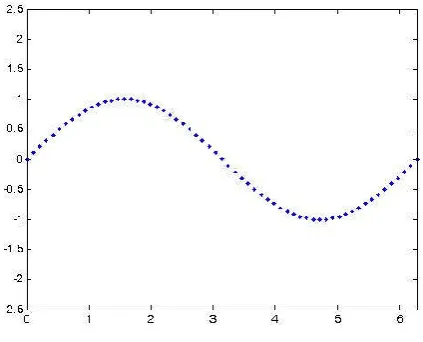
Example [58]: the following sample dataset A comes from the sine function which contained 60 points as shown in Fig. 1.

Fig. 1. Sample dataset A generated by the sine function

In the following experiments, we will approximate the dataset using traditional single hidden layer feed-forward neural networks with different number of hidden neurons trained by BP (Back Propagation) algorithm. Although there are many variants of BP algorithm, a faster BP algorithm called Levenberg-Marquardt is used in our experiments due to its faster convergence rate. All the experiments are carried out in MATLAB 7.10 (R2010a) environment running on an Intel(R) Core(TM) i3-2120 3.30GHz CPU. We will use 54 points of the dataset to train the neural networks and the other 6 points to test the un-optimized and the optimized networks.

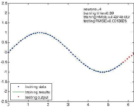
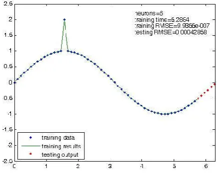
In Fig. 2, the neural network only needs 4 hidden neurons, based on the experience, to fit the function very well with 0.39 CPU training time (second), training RMSE and 0.0013825 testing RMSE.

Fig. 2. Results of training and testing with 4 hidden neurons using dataset A

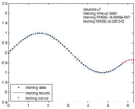
Fig. 4. Results of second training and testing with 7 hidden neurons using dataset A

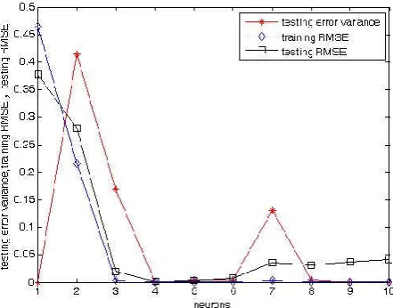
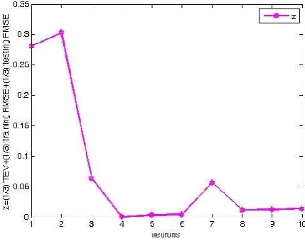
In the following experiments, on the same dataset A, for every number of neurons between 1 and 10 , we will train 20 NNs and compute the following index: training and testing root mean square error (RMSE)

2 0 1 ( ( ) ) 1 n i i i

RMSE f x y

n 

 





testing error variance (TEV)

1 1 1 2 1 ( ) 1 1 ( ( ) ) 1 1 ( )

1, , ; 1, ,

ij j ij

n n

i ij j ij

j j n i i m i i

error f x y

mean error f x y

n n

mean mean

m

TEV mean mean

m

i m j n

             









where yijis the output of xjin the i-th training NNs.

Fig. 5. The statistics performance of 20 NNs for each number of hidden neurons using dataset A If we add a noise to the dataset A, we can get sample dataset B which comes from function

1

s i n

2 ( )

2 2 x x

y f x

x



 

 



  

 _

 

(8)

and also contains 60 points as shown in Fig.6.

Fig. 6. Sample dataset B generated by the function yf x₁( )

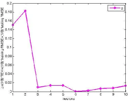
error (RMSE). The results are exhibited in Fig. 7 in which we can find the optimized NNs architecture for the dataset A is 6 hidden neurons because of the noise. Then we use the optimized NNs architecture with 6 hidden neurons to train a NNs which can fit the dataset B very well and have good generalization in Fig. 8.

Fig. 7. The statistics performance of 20 NNs for each number of hidden neurons using dataset B

4.

Multi-objective Optimization Model for NNs Architecture

There are many good theoretical results [36, 59-61] on the number of neurons in an optimized NNs architecture related to the function complexity under the sample datasets, which have helped much to understand certain issues regarding the properties of feed-forward neural networks but unfortunately at the time of practical implementations the bounds are loose or difficult to compute. Based on the above analysis, comprehensively considering of the above factors, in this paper, a multi-objective optimization model was built to find the optimized NNs architecture as follows: 1 2 0 1 1 1 2 1 min min min

. : (x) (w .x )

1 ( ( ) ) 1 ( ) 1 1 ( ( ) ) 1 1 ( )

1, , ; p

k k k

k

n

i i

i

ij j ij

n n

i ij j ij

j j n i i m i i training RMSE testing RMSE TEV

st NNs NN c b

RMSE f x y

n

error f x y

mean error f x y

n n

mean mean

m

TEV mean mean

m

i m j

                     













( ) / 4

2 / (5 * ( )) n

neurons p a b p Z

a N M

b T N M

                                       (9)

where yij is the output of xj in the i-th training NNs, k is the number of hidden neurons.

In this model, we will find an optimized NNs which hold three objective, minimal

training RMSE, testing RMSE and TEV, which has the best generalization and stability. The searching interval [ , ]a b can be determined by the following analysis: Some have a theoretical formulation behind, but others are just justified based on experience. The following notation is used: N is the input dimension of the data, Nh represents the

number of hidden neurons in the single hidden layer used in the neural architectures and

M is used for the output dimension (taken as 1 for all the problems considered). T is used to indicate the number of available training vectors. The following approaches described below correspond to two widely used software frameworks Weka [62] and Neuralware [63].

estimates by default the architecture size as Nh(NM) / 2 . It is not clear the justification for the introduction of this rule that has been also suggested in other works [64]. Based on experimental results, it seems that Weka suggests it based on its simplicity and on previous experience. Neuralware is another well-known commercial implementation of artificial neural networks. They suggest architecture with

/ (5 * ( )) h

N T NM neurons. Because T is commonly very large, we have: / (5 * ( )) ( ) / 2

T NM  NM (10)

So we take a_(NM) / 4_ and b_2 / (5 * (T NM))_, that means the optimized number of hidden neurons can be found in [ , ]a b.

There are many approaches to solve the multi-objective optimization problems [65] such as weighted sum approaches [66], lexicography approaches [67] and Pareto approaches [68] etc.

In this paper, weighted sum approach was used to convert multi-objective optimization to single objective optimization, and we simply selected the weight

1 / 3 1, 2,3 i

w  i . Then we get the single objective optimization model as follows:

1 2 0 1 1 1 2 1

1 1 1

min

3 3 3

. : (x) (w .x )

1 ( ( ) ) 1 ( ) 1 1 ( ( ) ) 1 1 ( ) 1, , p

k k k

k

n

i i

i

ij j ij

n n

i ij j ij

j j n i i m i i

z training RMSE testing RMSE TEV

st NNs NN c b

RMSE f x y

n

error f x y

mean error f x y

n n

mean mean

m

TEV mean mean

m i                        













; 1, ,

[ , ],

( ) / 4

2 / (5 * ( ))

m j n

neurons p a b p Z

a N M

b T N M

                       _           _{  }    (11)

In order to prove the existence of the optimized solution for this model, we first introduce some previous works on approximation of functions by NNs, and then we will prove the theorem of the existence and uniqueness of optimized solution.

There are many good results on approximation to continuous functions and dataset by neural networks using traditional algorithm such as BP, ELM, SVM and some constructive approaches.





( ) (w.x ) : , w,x ,

d _{span b b} d

     



Then d( )

N   if and only if

0

(x) ( x )

n

j j j

j

NN cw b







where cj, j0, ,n are real numbers and n is a positive integer.

We say that  is a sigmoid function, if it verifies tlim ( )t 0 and lim ( ) 1tt  , then (12) is called single-layer feed-forward neural network. If(x)( x-x )0 xRd, we

call (x) RBF (Radical Basis Function) function, then (12) is called RBF (Radical Basis Function) neural networks.

In the case of continuous functions we have the following density results Theorem 1 ([69) Let C( )R . Then



C R in the topology of uniform convergence on compact if and only if



Corollary 1 ([70]) (x) ( d)

yf C R can be approximated by a simplest neural networks (such as with Minimum number of hidden neurons).

In the case of not necessarily continuous functions we also have some density results. Theorem 2 ([71]) Let  be bounded, measurable and sigmoidal. Then



([0,1] )d

L .

The following theorem is a generalization of the above results.

Theorem 3 ([72]) Let



p b

a x dx 



Then for any function p( ) ( 1)

fL K p and every0, there is a network N



such that

,

K p

Nf  ₍₁₄₎

where

1 , ( ( ) )

p p

K p K

g 



For RBF neural networks we have the following results.

Theorem 4 ([73]) Let



fL R p and

every 0, there is a network N



p

Nf  (15)

where

1

( ( )p )p p

g 



There are some constructive approaches for function approximation. Theorem 5 ([41]) 1. Let x [ , ]k k

a b

 R , and f(x) be a multivariate continuous function , x [ , ]k

i a b i0,1, ,n be an uniform grid partition to [ , ] k

[ , ]a b is divided to

s

x ,x , , x_n (

n



s

1 1 1

2 2

x_i x_i

k

b a b a

s n 

 

   ₍₁₆₎

2. A depends on n， that is AA n( ).

3. The real numbers

f

x

functionf(x), that isfif(x ),i i0,1, 2, ,n .

For each0, we can construct a decay RBF neural network W_a(x, ( ))A n , and there exists a function ( )A n and a natural number N such that , when nN, we have

(x) _a(x, , ( ))

f W n A n  (17)

for allx [ , ]k

a b

 _.

Based on above theorems, we can prove the following theorem about the existence and uniqueness of optimized solution.

Theorem 6 For a given dataset, there exists only oneoptimized solution for the multi-objective optimization model (11).

Proof, we will first prove that the feasible regionDis not empty.

We assume the sample dataset Sis came from a certain continuous function yf x( ), for each hidden neurons p[ , ]a b , from the density theorem1-4, we can find a NNs with

phidden neurons using various traditional algorithm such BP, ELM, SVM and some constructive approaches:

1

(x) (w .x )

p

k k k

k

NN c b







which has the minimal distance

,

K p

RMSE Nf ₍₁₉₎

So the feasible region Dof multi-objective optimization model (1) is not empty. Then, as the number of hidden neurons p[ , ]a b is an integer, the searching interval is finite, which makes the multi-objective optimization model (11) have only one optimized solution for the certain sample datasetS.□

Based on theorem 6 we can get the following algorithm to solve the above multi-objective optimization model:

Algorithm 4.1: Multi-objective Optimization Algorithm for Optimized Neural Network Architecture Avoiding

Overfitting (ONNAAO)

Input: the training and testing dataset.

Output: the optimized neural network architecture or number of hidden neurons of NNs.

Step 1: based on the input data, compute the searching interval [a, b], = ⌈( + )/4⌉, = ⌈2 /(5 ∗ ( + ))⌉. N is the input dimension of the data, and M is the output

dimension Step 2:

for i = a to i = b

for j = 1 to j = m,

train a neural network with i hidden neurons using Levenberg-Marquardt algorithm for the training dataset.

Step 3:

for each trained neural network,

compute training RMSE, testing RMSE and TEV, then z = 1/3(training RMSE + testing RMSE + TEV)

Step 4: determine the optimized neural network

architecture or number of hidden neurons of NNs based on the minimal z.

Step 5: construct an optimized NNs with minimal z to training and forecasting the stock indexes.

Although there are many algorithms to train the NNs, in this paper, we use Levenberg-Marquardt BP algorithm for the all experiments, due to its faster convergence rate.

For above datasets AandB, using the algorithm 4.1 we can get the results of Fig.9 and Fig. 10. In Fig. 9, we can see that the optimized value is 4 hidden neurons for the dataset A, and in Fig. 9, we can see that the optimized value is 6 hidden neurons for the dataset B.

Fig. 10. The results for dataset B, optimized value is 6

5.

Experiments on Stock Data

All stock market trends are fast changing. They are affected by not only the individual investors and many institutional investors, but also impacted by domestic political, economic situations and many other factors. Therefore, it is very difficult to build a classical parameter model to predict the market movement [46]. But it is easy to build a NNs model to fit the stock dataset, and the choice of optimized neural network architecture is still a problem that has not been solved yet. In this section, we will use above multi-objective optimization algorithm to build an optimized neural network architecture model to predict Chinese Shanghai Composite Index.

We first collected the sample data of Chinese Shanghai Composite closing Index from internet stock database. The collection period is from November 25, 2015 to January 16, 2017 and the number of data totaled 280 (Fig. 11).

We will use 275 points of the dataset to train the neural networks and the other 5 points to test the old and the optimized networks.

Fig. 11. Chinese Shanghai Composite closing Index in 280 days

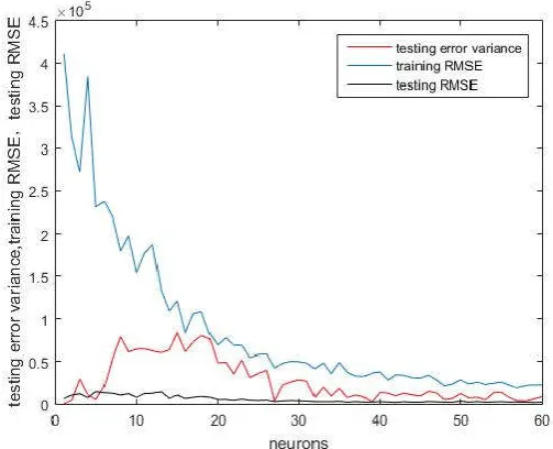
Fig. 13. The result for the stock dataset, optimized value is 57

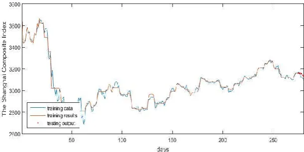
In the end, we built a neural network with 57 hidden neurons, and trained it with 275 Chinese Shanghai Composite closing Index using Levenberg-Marquardt BP algorithm, and predicted the last 5 as it is shown in Fig. 14. Fig.15 is the enlarged part of the predicted values.

Fig. 15. The enlarged part of the predicted values

The results of these experiments are presented in table 1.

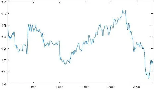
We collected another dataset: Jinlong Automobile (600686) from April 19, 2016 to June 13, 2017, a total of 280 days closing price as shown in Figure 16.

Fig. 16. A total of 280 days closing price of Jinlong Automobile (600686) from April 19, 2016 to

June 13, 2017, in 280 days

Fig. 17. The three objective value in the searching process

In the end, we built a neural network with 62 hidden neurons, and trained it with 275 closing price of Jinlong Automobile (600686) from April 19, 2016 to June 13, 2017, in 280 days, using Levenberg-Marquardt BP algorithm, and predicted the last 5 as it is shown in Fig.19. Fig.20 is the enlarged part of the predicted values.

The experimental results are summarized in Table 1.

Fig. 19. The application of the optimized NNs for prediction

Table 1. Results above experiments

Dataset (number)

Come from

Searching interval

Number of experiments for each NNs

Optimal value of hidden neurons A(60)

sin

y x [1,10] 20 4

B(60)

1( )

y f x [1,10] 20 6

S(280) Chinese Shanghai Composite closing Index

[1,60] 20 57

J(280) closing price of Jinlong Automobile (600686)

[1,70] 20 62

6.

Performance Comprehensive Comparison with Traditional

Algorithms

In this section, in order to illustrate the originality, novelty and superiority of the presented algorithm (ONNAAO), we will make many numerical experiments for the problem of stock indexes prediction with theabove datasets, some performance of the presented algorithm, such as training time, training RMSE, testing RMSE and neurons, will be compared with the traditional algorithms such as AR, ARMA, ordinary BP, SVM.

In the following experiments, a faster BP algorithm called Levenberg-Marquardt algorithm is used, although there are many variants of BP algorithms. The SVM algorithm source codes aredownloaded from LIBSVM3.21 [74].

To compare the performance of the algorithms mentioned above, in each experiment 30 trials have been carried out for each algorithm and the average training time, the ratio of the average training time with ONNAAO average training time (RATT):

average training time of the traditional algorithms RATT

average training tim ofe ONNAAO



the average testing, the average testing RMSE, the testing standard deviations (Dev), and the ratio of the average testing RMSE with ONNAAO average testing RMSE (RATR):

average testing time of the traditional algorithms RATR

average trsting RMSE tim ofe ONNAAO



Table 2. Performance comparison for ONNAAO Algorithms Training

performance

Testing performance Parameters

Time RATT Average RMSE

Dev RATR

ONNAO 1.78975 1 96.9096 73.6057 1 Nodes=57

Ordinary BP 1.88548 1.0535 117.1466 106.9294 1.2088 Nodes=100

AR(p) 1.3634 0.7617 145.3068 20.12 1.4994 P=20

ARMA(p,q) 1.4735 0.8232 208.9682 78.9804 2.1563 P=20, q=15

SVM 2.5364 1.4171 765.3969 101.334 7.898 SVs=56

From the performance comparison in table 2, we can see that the proposed ONNAAO algorithm has the best average testing RMSE, although the running time of ONNAAO is not the shortest, which fully shows that the ONNAAO algorithm has better prediction accuracy in performance compared with traditional prediction algorithms. Although in the forecasting problem there are also some approaches [4, 42,48] with the hybrid algorithms such as neural networks combined with some other techniques, wavelets for example, but the ONNAAO algorithm is relatively simple and intuitive.

Remark 1. The training and testing time of ONNAAO are the time of training and testing after determining the number of hidden neurons for optimized neural network architecture.

7.

Conclusions

In this paper, our goal is to find the optimized neural networks architecture and reduce the over-fitting phenomenon. Firstly, we analyzed the reasons for over-fitting and instability of NNs. Then we consider minimizing three objective indexes: training and testing root mean square error (RMSE) and testing error variance (TEV). Lastly we built a multi-objective optimization model, then convert to single objective optimization model to find the optimized NNs architecture. At the same time, the existence and uniqueness theorem 6 of optimized solution is proved. And an algorithm for Optimized Neural Network Architecture Avoiding Overfitting (ONNAAO) is constructed to training and forecasting two stock closing price datasets. Lastly, some performance such as training time, testing RMSE and neurons, has been compared with the traditional algorithm (AR, ARMA, ordinary BP, SVM) through many numerical experiments, which fully verified the better prediction accuracy, correctness and validity of the theory.

Acknowledgement. This work was supported by the National Natural Science Foundation of

References

1. Stock, J.H. and M.W. Watson, A probability model of the coincident economic indicators. 1988, National Bureau of Economic Research Cambridge, Mass.,USA.

2. Tang H, Chiu K C, Xu L. Finite mixture of ARMA-GARCH model for stock price prediction. Proceedings of the Third International Workshop on Computational Intelligence in Economics and Finance (CIEF'2003), North Carolina, USA. 2003: 1112-1119..

3. Ince, H. and T.B. Trafalis, Kernel principal component analysis and support vector machines for stock price prediction. IIE Transactions, 2007. 39(6): p. 629-637.

4. Muzhou, H., C. Ming, and Z. Yangchun, A Self-Organizing Mixture Extreme Leaning Machine for Time Series Forecasting, in Proceedings of ELM-2014 Volume 1. 2015, Springer. p. 225-236.

5. Palm, R.B. Prediction as a candidate for learning deep hierarchical models of data. 2012; Available from: https://github.com/rasmusbergpalm/DeepLearnToolbox.

6. Sun, J., H. Li, and H. Adeli, Concept Drift-Oriented Adaptive and Dynamic Support Vector Machine Ensemble With Time Window in Corporate Financial Risk Prediction. Ieee Transactions on Systems Man Cybernetics-Systems, 2013. 43(4): p. 801-813.

7. Metzger, A., et al., Comparing and Combining Predictive Business Process Monitoring Techniques. Ieee Transactions on Systems Man Cybernetics-Systems, 2015. 45(2): p. 276-290.

8. Anagnostopoulos, C. and S. Hadjiefthymiades, Intelligent Trajectory Classification for Improved Movement Prediction. Ieee Transactions on Systems Man Cybernetics-Systems, 2014. 44(10): p. 1301-1314.

9. Liu F, Wang J. Fluctuation prediction of stock market index by Legendre neural network with random time strength function. Neurocomputing, 2012, 83: 12-21.

10. Hippert, H.S., C.E. Pedreira, and R.C. Souza, Neural networks for short-term load forecasting: A review and evaluation. Power Systems, IEEE Transactions on, 2001. 16(1): p. 44-55.

11. Maier, H.R. and G.C. Dandy, Neural networks for the prediction and forecasting of water resources variables: a review of modelling issues and applications. Environmental modelling & software, 2000. 15(1): p. 101-124.

12. Han, M. and Y. Wang, Analysis and modeling of multivariate chaotic time series based on neural network. Expert Systems with Applications, 2009. 36(2): p. 1280-1290.

13. Huang, W., et al., Neural networks in finance and economics forecasting. International Journal of Information Technology & Decision Making, 2007. 6(01): p. 113-140.

14. Xie J X, Cheng C T, Chau K W, et al. A hybrid adaptive time-delay neural network model for multi-step-ahead prediction of sunspot activity. International Journal of Environment and Pollution, 2006, 28(3-4): 364-381.

15. Lapedes, A. and R. Farber, Nonlinear signal processing using neural networks: Prediction and system modelling. 1987.

16. Zhang, G.P., A neural network ensemble method with jittered training data for time series forecasting. Information Sciences, 2007. 177(23): p. 5329-5346.

17. Yu, S.W., Forecasting and arbitrage of the Nikkei stock index futures: an application of backpropagation networks. Asia-Pacific Financial Markets, 1999. 6(4): p. 341-354.

18. Yu Z, Song S, Duan G, et al. The Design of RBF Neural Networks for Solving Overfitting Problem. Intelligent Control and Automation, 2006. WCICA 2006. The Sixth World Congress on. IEEE, 1: 2752-2756.

19. Lawrence S, Giles C L. Overfitting and neural networks: conjugate gradient and backpropagation. Neural Networks, 2000. IJCNN 2000, Proceedings of the IEEE-INNS-ENNS International Joint Conference on. IEEE, 2000, 1: 114-119.

21. Schittenkopf, C., G. Deco, and W. Brauer, Two strategies to avoid overfitting in feedforward networks. Neural Networks, 1997. 10(3): p. 505-516.

22. Cunningham, P., J. Carney, and S. Jacob, Stability problems with artificial neural networks and the ensemble solution. Artificial Intelligence in Medicine, 2000. 20(3): p. 217-225. 23. Gómez, I., L. Franco, and J.M. Jerez, Neural network architecture selection: Can function

complexity help? Neural processing letters, 2009. 30(2): p. 71-87.

24. Wright J L, Manic M. Neural network architecture selection analysis with application to cryptography location. Neural Networks (IJCNN), The 2010 International Joint Conference on. IEEE, 2010: 1-6.

25. Lawrence, S., C.L. Giles, and A.C. Tsoi, What size neural network gives optimal generalization? Convergence properties of backpropagation. 1998.

26. Perrone, M.P. and L.N. Cooper, When networks disagree: Ensemble methods for hybrid neural networks. 1992, DTIC Document.

27. Tay F E H, Cao L. Application of support vector machines in financial time series forecasting. Omega, 2001, 29(4): 309-317.

28. Doan C D, Liong S. Generalization for multilayer neural network Bayesian regularization or early stopping. Proceedings of Asia Pacific Association of Hydrology and Water Resources 2nd Conference. 2004: 5-8..

29. Hagiwara, K. and K. Fukumizu, Relation between weight size and degree of over-fitting in neural network regression. Neural Networks, 2008. 21(1): p. 48-58.

30. Murata, N., S. Yoshizawa, and S. Amari, Network information criterion-determining the number of hidden units for an artificial neural network model. Neural Networks, IEEE Transactions on, 1994. 5(6): p. 865-872.

31. Akaike H. Information theory and an extension of the maximum likelihood principle. Selected Papers of Hirotugu Akaike. Springer New York, 1998: 199-213.

32. Moody J. The Effective Number of Parameters: An Analysis of Generalization and Regularization in Nonlinear Systems, this volume. Advances in Neural Information Processing Systems, 4.

33. Vapnik V. The nature of statistical learning theory. Springer science & business media, 2013. 34. Ripley B D. Pattern recognition via neural networks. A volume of Oxford Graduate Lectures

on Neural Networks, title to be decided. Oxford University Press, 1996.

35. Baum, E.B. and D. Haussler, What size net gives valid generalization? Neural computation, 1989. 1(1): p. 151-160.

36. Barron, A.R., Approximation and estimation bounds for artificial neural networks. Machine Learning, 1994. 14(1): p. 115-133.

37. Yuan H C, Xiong F L, Huai X Y. A method for estimating the number of hidden neurons in feed-forward neural networks based on information entropy. Computers and Electronics in Agriculture, 2003, 40(1): 57-64.

38. Liu, Y., J.A. Starzyk, and Z. Zhu, Optimizing number of hidden neurons in neural networks. eeC, 2007. 1(1): p. 6.

39. Carney J, Cunningham P. The NeuralBAG algorithm: optimizing generalization performance in bagged neural networks. ESANN. 1999: 135-140.

40. Breiman, L., Bagging predictors. Machine Learning, 1996. 24(2): p. 123-140.

41. Hou, M. and X. Han, Constructive approximation to multivariate function by decay RBF neural network. Neural Networks, IEEE Transactions on, 2010. 21(9): p. 1517-1523. 42. Muzhou, H. and H. Xuli, The multidimensional function approximation based on

constructive wavelet RBF neural network. Applied Soft Computing, 2011. 11(2): p. 2173-2177.

43. Muzhou, H., H. Xuli, and G. Yixuan, Constructive approximation to real function by wavelet neural networks. Neural Computing & Applications, 2009. 18(8): p. 883-889.

SYSTEMS PART 1 FUNDAMENTAL THEORY AND APPLICATIONS, 2002. 49(12): p. 1876-1879.

45. Xi, L., et al., A new constructive neural network method for noise processing and its application on stock market prediction. Applied Soft Computing, 2014. 15: p. 57-66. 46. Huang C J, Chen P W, Pan W T. Using multi-stage data mining technique to build forecast

model for Taiwan stocks. Neural Computing and Applications, 2012, 21(8): 2057-2063. 47. Oh, K.J. and K. Kim, Analyzing stock market tick data using piecewise nonlinear model.

Expert Systems with Applications, 2002. 22(3): p. 249-255.

48. Adhikari, R. and R.K. Agrawal, Forecasting strong seasonal time series with artificial neural networks. Journal of Scientific & Industrial Research, 2012. 71(10): p. 657-666.

49. Huang, G.B., Learning capability and storage capacity of two-hidden-layer feedforward networks. Ieee Transactions on Neural Networks, 2003. 14(2): p. 274-281.

50. Soyguder, S., Intelligent control based on wavelet decomposition and neural network for predicting of human trajectories with a novel vision-based robotic. Expert Systems with Applications, 2011. 38(11): p. 13994-14000.

51. Zhang, G., B. Eddy Patuwo, and M. Y Hu, Forecasting with artificial neural networks:: The state of the art. International journal of forecasting, 1998. 14(1): p. 35-62.

52. Zevallos, M., B. Santos, and L.K. Hotta, A note on influence diagnostics in AR(1) time series models. Journal of Statistical Planning and Inference, 2012. 142(11): p. 2999-3007.

53. Cabana, A., E.M. Cabana, and M. Scavino, Weak Convergence of Marked Empirical Processes for Focused Inference on AR(p) vs AR(p+1) Stationary Time Series. Methodology and Computing in Applied Probability, 2012. 14(3): p. 793-810.

54. Flores, J.J., M. Graff, and H. Rodriguez, Evolutive design of ARMA and ANN models for time series forecasting. Renewable Energy, 2012. 44: p. 225-230.

55. Song, P.X.K., et al., Statistical analysis of discrete-valued time series using categorical ARMA models. Computational Statistics & Data Analysis, 2013. 57(1): p. 112-124. 56. Purwanto, C. Eswaran, and R. Logeswaran, An enhanced hybrid method for time series

prediction using linear and neural network models. Applied Intelligence, 2012. 37(4): p. 511-519.

57. Yan, W.Z., Toward Automatic Time-Series Forecasting Using Neural Networks. Ieee Transactions on Neural Networks and Learning Systems, 2012. 23(7): p. 1028-1039. 58. Muzhou, H. and M.H. Lee, A New Constructive Method to Optimize Neural Network

Architecture and Generalization. arXiv preprint arXiv:1302.0324, 2013

59. Camargo, L. and T. Yoneyama, Specification of training sets and the number of hidden neurons for multilayer perceptrons. Neural computation, 2001. 13(12): p. 2673-2680. 60. Scarselli, F. and A. Chung Tsoi, Universal approximation using feedforward neural

networks: A survey of some existing methods, and some new results. Neural Networks, 1998. 11(1): p. 15-37.

61. Simon, H., Neural networks: a comprehensive foundation. 1999: Prentice Hall.

62. Witten, I.H. and E. Frank, Data Mining: Practical machine learning tools and techniques. 2005: Morgan Kaufmann.

63. Jack Copper, J.W., Alex Kulik, Carolyn Osmond, Bob Everly Neuralware I :The reference guide. http://www.neuralware.com, 2001.

64. Piramuthu, S., M.J. Shaw, and J.A. Gentry, A classification approach using multi-layered neural networks. Decision Support Systems, 1994. 11(5): p. 509-525.

65. Deb, K., Multi-objective optimization. Search Methodologies, 2005: p. 273-316.

66. Marler, R.T. and J.S. Arora, The weighted sum method for multi-objective optimization: new insights. Structural and multidisciplinary optimization, 2010. 41(6): p. 853-862.

67. Marler, R.T. and J.S. Arora, Survey of multi-objective optimization methods for engineering. Structural and multidisciplinary optimization, 2004. 26(6): p. 369-395.

69. Pinkus, A., Approximation theory of the MLP model in neural networks. Acta Numerica, 1999. 8(1): p. 143-195.

70. Mulero-Martínez, J.I., Best approximation of Gaussian neural networks with nodes uniformly spaced. Neural Networks, IEEE Transactions on, 2008. 19(2): p. 284-298. 71. Cybenko, G., Approximation by superpositions of a sigmoidal function. Mathematics of

Control, Signals, and Systems (MCSS), 1989. 2(4): p. 303-314.

72. Burton, R.M. and H.G. Dehling, Universal approximation in p-mean by neural networks1. Neural Networks, 1998. 11(4): p. 661-667.

73. Park, J. and I.W. Sandberg, Universal approximation using radial-basis-function networks. Neural computation, 1991. 3(2): p. 246-257.

74. Lin, C.C.C.a.C.J. LIBSVM -- A Library for Support Vector Machines. Available from: https://www.csie.ntu.edu.tw/~cjlin/libsvm/.

Zhou Tao, 38 years old, is a PhD candidate in service at school of business administration, South China University of Technology, China. And His current research interests include machine learning, computational intelligence, neural networks, revenue management and green operation management. Contact him at [email protected]

Hou Muzhou received the B.S. degrees from Hunan Normal University, Changsha, China, M.S. and Ph.D. degree from Central South University, Changsha, China in 1985, 2002, and 2009, respectively. He is currently a Professor and doctorial advisor in School of Mathematics and Statistics, Central South University, PR China. His current research interests include machine learning, computational intelligence, neural networks, data mining and numerical approximation.

Liu Chunhui is a PhD candidate in service at school of business administration, South China University of Technology, China. His current research interests include neural networks, queuing theory, revenue management and green operation management. Contact him at [email protected]