A Lane-Changing Behavioral Preferences Learning Agent with its Applications

(1)

A Lane-Changing Behavioral Preferences

Learning Agent with its Applications

Wang Jian1,3, Cai Baigen1,2, Liu Jiang1,2, and Shangguan Wei1,3

1 _{School of Electronical and Information Engineering} Beijing Jiaotong University, Beijing 100044, China

[email protected] 2

State Key Laboratory of Rail Traffic Control and Safety Beijing Jiaotong University, Beijing 100044, China 3

Beijing Engineering Research Center of EMC and GNSS Technology for Rail Transportation

Beijing 100044, China

Abstract. Traditional lane-changing (LC) behavioral researches usually focus on

the driver’s cognitive performance which includes the driver’s psychological and be-havioral habit characteristics, rarely involving the affection of expert driver’s com-prehensive behavioral preferences, such as: safety and comfort performance in LC process. Towards the free LC process, a novel LC safety and comfort degree index is proposed in this paper, as well as, the novel definition of LC driving behavioral pref-erences is described in detail. Taking advantage of interactive evolutionary comput-ing (IEC) and real-time optimization (RTO) metrics, a kind of LC behavioral pref-erences on-line learning agent extending traditional Belief-Desire-Intention (BDI) structure is explicitly proposed, which can perform behavioral preferences learn-ing activities in the LC process. In addition, drivlearn-ing behavioral preferences learnlearn-ing strategies are introduced which can gradually grasp essentials in driver’s subjective judgments in decision-making of the LC process and make the LC process more safety and scientific. Specifically, a conceptual model of the agent, driving behav-ioral preferences learning-BDI (DpL-BDI) agent is introduced, along with corre-sponding functional modules to grasp driving behavioral preferences. Furthermore, colored Petri nets are used to realize the components and scheduler of the DpL-BDI agents. In the end, to compare with the traditional LC parameters’ learning methods (such as: the least squares methods and Genetic Algorithms), a kind of LC problems is suggested to case studies, testing and verifying the validity of the contribution.

Keywords:Agent, Driving behavioral preferences, Interactive learning, Colored

Petri Nets (CPN).

1. Introduction

(2)

Currently, majority of lane-changing (LC) modeling methods’ researches are con-cerned with theoretical relevance and simulation issues. Rahman et al. conducted a de-tailed review and systematic comparison of existing microscopic LC models that are re-lated to roadway traffic simulation to provide a better understanding of respective prop-erties, including strengths and weaknesses of the LC models, and to identify potential for model improvement using existing and emerging data collection technologies [26]; Zheng comprehensively reviewed recent developments in modeling LC behavior and categorized the major LC models in the literature into two groups: models that aim to capture the LC decision-making process, and models that aim to quantify the impact of LC behavior on surrounding vehicles [39].

Therein, towards the driving safety [19][15] and comfort performance [14][23][21] assessment, the three risk indicators (time-to collision (TTC), time headway (TH), and safety margin (SM)) and some scales (such as: driving comfort scales (DCS), perceived driving abilities (PDA) scale, situational driving avoidance (SDA) scales, et al.) are re-spectively employed in a large scale. However, how to construct the LC decision-making problems constrained with the driving behavioral preferences still represents a challenge. Therein, agents are effective methods to construct the human-computer interaction (HCI) model. Sardina & Padgham developed a typical BDI-style agent-oriented program-ming language that enhances usual BDI programprogram-ming style with three distinguished fea-tures: declarative goals, look-ahead planning, and failure handling [28]. Additionally, Wu et al. presented a new-complete first-order temporal BDI logic and forest multi-agent sys-tem and shown how to characterize the forest multi-agent syssys-tem by using the hierarchical structure of modules [34]. Nonetheless, there is little literature focus on establishing the LC driving behavioral preferences interactive learning agent.

In order to effectively perform human-computer interactions in the LC process, this paper proposes a novel driving behavioral preferences’ definition to study the driving be-havioral preference’s influence on the LC process, which includes the safety and comfort performance assessment methods. A new kind of interactive driving behavioral prefer-ences learning agent based on (Belief, Desire and Intention) BDI structures is established. Under the real-time optimization (RTO) [4][1] framework, driving behavioral preference learning algorithms are proposed in this paper. Conceptual agent models and correspond-ing functional modules are explicitly introduced along with preference learncorrespond-ing algo-rithms. Colored Petri nets are employed to realize and analyze the agent.

The remainder of this paper is organized as follows: Section2 reviews related re-searches on LC driving behavioral preferences learning. Section 3 presents the basic free LC models, as well as the proposes the free LC MADM problems. In Section 4, the def-inition of free LC driving behavioral preferences is proposed, as well as, the DpL-BDI agent’s conceptual model with its corresponding functional modules and associated al-gorithms is explicitly introduced. Section 5 presents an approach of how to apply the interactive learning agents in LC process. Section 6 concludes the article and assesses the future perspectives.

2. Related work

(3)

perfor-mance assessment methods in the early period to current researches on the LC driving behavioral preferences. A lot of new technologies and intelligent optimization algorithms are widely applied to identify the parameters of LC model and the LC driving behavioral preferences, such as: the least squares methods, genetic algorithm [8] etc. This section not only summaries recently published researches on LC driving behavioral preferences but also focuses on learning methods based on human-computer interaction.

Lane-changing’s model and performance- Currently, lane-changing (LC) researches become a new-emerging research issue that targets the quantitative relations of the driv-ing process. Specifically, Laval & Leclercq introduced a framework to solve this problem using a macroscopic theory of vehicle LC inside microscopic models, as well as, in their theory, lane changes take place according to a stochastic process that has been validated in the field, and whose mean value is a function of lane-specific macroscopic quantities [17]; Jin proposed a simple model for studying bottleneck effects of LC traffic and ag-gregate traffic dynamics of a roadway with LC areas [9]; Jin considered weaving and non-weaving vehicles as two commodities and develop a multi-commodity, behavioral Lighthill-Whitham-Richards (LWR) model of LC traffic flow and derive a fundamental diagram with parameters determined by LC and LC characteristics as well as road ge-ometry and traffic composition [10]; Zheng et al. proposed a neural network (NN) model to capture the complexity of LC, and large-scale trajectory data are employed for model estimation and validation [38]; Lv et al. developed an integrative traffic model, in which a method to calculate the LC probability and the merging probability was proposed [20]; Patire & Cassidy introduced a key mechanism of the vehicular LC: LC can be induced by speed disturbances (SDs) that periodically arise in the expressway’s median and center lanes [25]. It is conceivable that how to comprehensively quantify the driving behavioral preferences with the safety and comfort performance in the ITS’ models still remains a challenge.

Driving behavioral preferences- Alternatively, a lot of researches are concerned with the relations between driving behavior and the performance of LC process. For example, Hidas introduced the Simulation of Intelligent TRAnsport Systems (SITRAS), a massive multi-agent simulation system in which driver-vehicle objects are modeled as autonomous agents [6]; Tang et al. proposed a macroscopic model of LC that is consistent with LC be-havior on a two-lane highway [31]; Tideman et al. presented a new approach for determin-ing users’ preferences and finddetermin-ing the best compromise between those preferences when designing a new driver support system [32]; Schubert et al. described a system that can perceive the vehicle’s environment, assess the traffic situation, and give recommendations about lane-change maneuvers to the driver [29]; Peng et al. built a new cellular automaton (CA) model, based on the driving decision (DD), as well as, in the DD model, a driver’s decision is divided into three stages: decision-making, action, and result [37]; Zheng et al. investigated the effects of LC in driver behavior by measuring (i) the induced transient behavior and (ii) the change in driver characteristics and the changes in driver response time and minimum spacing. Nonetheless, these researches need the large scale samples, suffering the approaches to grasp the driving behavioral preferences based evolutionary strategies [40].

(4)

models [5][7][22][33]. Typically, BDI (Belief, Desire and Intention) agent models are extensively employed to demonstrate rational reasoning abilities of agents, attracting in-creasing attention in both academia and application fields recently. For example, Casalia et al. introduced a graded BDI agent development framework and proposed a sound and complete logical framework for it [3]. Thereafter, a lot of agent’s applications [27][35][13] are developed. However, the applications rarely involved the driving behavioral prefer-ence. Meanwhile, the Petri nets are usually employed to establish agent models [18][24]. At present, little literature reported the methods in establishing the driving behavioral preferences learning agent.

Parameters identification-With the development of probe vehicle technologies and the emerging connected vehicle technologies, applications and models using trajectory data for calibration and validation significantly increase. Traditional parameters’ identification based vehicle trajectory always focuses on the car-following process. Jin et al. proposed the error dynamic model based on an acceleration-based generic car-following model formulation, as well as, they explore the mechanism and countermeasures of the error accumulation problems of car-following models calibrated with microscopic vehicle tra-jectory data[12]; to deal with traveler behaviors in transport studies, Kim et al. proposed a rigorous methodology to calibrate a GM-type car-following model with random coeffi-cients, which could account for the heterogeneity across drivers who respond differently to stimuli [12]. In addition, the lane changing process can be divided into two coordinates: horizontal and vertical motion model, as well as, the horizontal motion model can be re-garded as a car-following process. Because the lane changing process is complex, there is little literature reports the related parameters’ interactive learning methods.

Thereafter, a novel driving behavioral preferences’ definition and a new kind of inter-active driving behavioral preferences learning agent based on (Belief, Desire and Inten-tion) BDI structures are proposed to study the driving behavioral preference’s influence on the LC process.

3. The mathematical formulation of Lane-changing

3.1. The free Lane-changing model

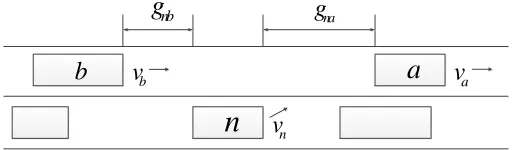
The classical free Lane-changing (LC) model (in [26][39]) is presented as follows in Fig. 1:

gD

na=max{gaD, gDa +βDa1vn+βaD2(vn−va) +εna}

gD

nb=max{g D b , g

D b +β

D

b1vb+βbD2(vn−vb) +εnb}

Where,gDnais critical lead gap;gnbD is critical lag gap;g

D

a is minimum lead gap;gbD

is minimum lag gap;va is speed of the lead vehicle;vbis speed of the lag vehicle;vn is

speed of the lane changer;βare parameters,εna,εnbare error terms.

The acceleration of the lane changer is:

dvj−1(t)

dt =h[v(∆xj(t))−vj−1(t)] +τ(∆vj(t)) (1)

where,∆xj(t)is described as the distance between the lead car and the participant car,

(5)

b

a

n

nb

g

_na

b

v

_a

n

v

Fig. 1.The classical free Lane-changing model

the two vehicles; vj−1(t)was the speed of participant car at the timet, ∆vj(t)is the

relative speed of the two vehicles(∆vj(t) =vj(t)−vj−1(t)),his the synthesized index

corresponding to the safety and economy performance, τ is the delay factor, j is the

vehicle number.

Nonetheless,v(∆xj(t))in the formula is described as:

v(∆xj(t)) =

vj−1(t){1 +tanh[G(∆xj(t)−hc(t)]} ∆xj(t)< hc(t)

vj−1(t) + (vmax−vj−1(t))·tanh[G(∆xj(t)−hc(t))]∆xj(t)>hc(t)

(2)

where,hc(t)is described as a safe distance at timetbetween the two vehicles (To

simplify the study,hc(t)is defined as a constant),Gandhare both dynamic unknown

parameters,vmaxis the maximum freedom speed of the participant car,tanhis the dual

music function.

3.2. The free lane-changing multi-attribute decision-making (MADM) problems

The free lane-changing (LC) is a kind of uncertainty MADM problems involving human-computing interaction, where human’s preferences tend to be constraints of the decision solutions. Therefore, it is necessary to discuss the decision-making mechanism based on driver’s behavioral preference interactive learning in LC process.

(6)

OPT:

OBJno(x, y)< Ono, no= 1,2, ... (3)

s.t.

lane-changing model safety indicator comfort indicator

x∈R, y∈ {0,1}

µpre(x, y) =Driving−pref erence

Where,xandy are described as continuous and discrete operating variables(x ∈

R, y ∈ {0,1});Ono(no = 1,2, ...)are key quantitative objective;µpreis described as

fuzzy membership functions corresponding to the decision-making vectors, which reflects the decision-making behavioral preferences.

4. Driving behavioral preferences learning BDI (DPL-BDI) Agent

Towards the objective whose optimal values are unknown and dynamic, human usually tends to solve it by subjective experience. In addition, based on the definition of driving behavioral preferences, computer can track and learn the free LC multi-attribute decision-making (MADM) process, as well as make the driving process more personalized and comfortable.

Time to collision (TTC) [36][30] has been a key vehicle safety metric for decades. With the increasing prevalence of advanced driver assistance systems and vehicle automa-tion, TTC and many related metrics are being applied to the analysis of more complicated scenarios, as well as being integrated into automation algorithms.

The traditional TTC index [2] is described as follows:

T HWn =tn,l1−tn−1,l1 (4)

The time headway and vehicle speed can be determined:

Vn=

D

(Tn,L2−tn,L1)

(5)

Where,nrefers to the vehicle identification (assigned by the order of appearance),L1

is the upstream reference line,L2is the down stream reference line, andDcorresponds

to the distance between the two reference markings. The length of D used in this study is 15m.

The distance gap DX between two vehicles is determined by

DXn=T HWn×Vn−lcar (6)

Where,

the average car lengthlcaris taken to be 4.5 m.

TTC is then estimated using

T T Cn=

DX

DV = DX

vn−vn−1, vn> vn−1

(7)

While the TTC metric was originally conceived to be a mandatory constraint in the car-following process, its applications rarely involving the driver’s expectations for the TTC index based driving behavioral preferences within the safe consideration.

Definition 1(Lane-changing safety degree index):

SI=

q

1

N

PN

i=1(T T Ci−TT C¯ )2

ˆ

ξ (8)

Where,icorresponds to theithtime in the car-following process;T T Ci is the time

to collision index at theithtime in the car-following process;TT C¯ is described as the

averageT T Cindex;ξˆis the expected variance ofT T C.

Definition 2(Lane-changing comfort degree index):

CI =

q

1

N

PN

i=1(ai−¯a)2 ˆ

σ (9)

Where,icorresponds to theith_{time in the car-following process;}_a

iis the

participa-tion car’s acceleraparticipa-tion at theith_{time in the car-following process;}_¯_a_{is described as the}

average acceleration(ai);σˆis the expected variance of the acceleration.

Definition 3(Free Lane-changing driving behavioral preferences):

Towards the dynamic free lane-changing MADM problems, driver’s concern degree of safety and comfort performance are defined as driving behavioral preferences.

Driving behavioral preference is a two-tuple:Driving−pref erence = {Ei, λi}.

Where,iis the attributes’ number of the MADM problem. Only the safety and comfort

degree index are discussed in this paper, so,i= 2;Eiis described as the optimal value of

each attribute in the free LC MADM problems;λiis described as the weight coefficient

of each attribute in the free LC MADM problems.

4.1. Agent’s model and function

4.1.1. Conceptual model

Real-time optimization (RTO) [24][12], which refers to the online optimization of a process plant, RTO attempts to optimize process performance (usually measured in terms of profit or operating cost) thereby enabling companies to push the profitability of their processes to their true potential as operating conditions change. The control problem is solved apart from the optimization problem at different frequencies and using different models.

Based on real-time optimization (RTO) [24] theory, driving behavioral preferences learning can be transformed to a class of RTO problems whose conceptual model is shown in Fig. 2.

(8)

Fig. 2.Driving behavioral preferences learning conceptual model

4.1.2. Driving behavioral preference learning (DpL-BDI) Agent

In regard to traditional BDI models, Belief corresponds to the information that agents have about the goal and circumstance; Desire signifies the states of affairs that agents would wish to be brought; Intention indicates the desire that agents have committed to achieve. In this sense, driving behavioral preferences interactive learning models can be considered as that the agents can constantly update the driving behavioral preference states in achieving objectives and interacting with the driver by belief, desire and inten-tion.

In order to make the Agent have similar driving behavior and human preferences, interactive learning (L) and driving preferences (Dp) tuples are added in traditional BDI models to constitute DpL-BDI Agent model.

Definition 4(DpL-BDI models):

A DpL-BDI model is a five-tuple,DpL−BDI ={Dp, L, B, D, I}, where

1. Bis the Belief set, including the LC goals that agents wish to achieve and the related

data, i.e. forBi ∈ B we haveBi ={[gi, datai|gi ∈ G, datai ∈Data,}.Gis the

goal set,Datais the data set;

2. Dis the Desire set, including the assessments of agents’ achievements and related

data, i.e. forDi ∈ Dwe haveDi,Di ={[gei, dataj|gei ∈ GE, dataj ∈ Data}

(9)

3. I is the Intention set, including the algorithms that are employed to accommodate

Belief set and Desire set, i.e. forIi∈Iwe haveIi={ali(Di, Bi|ali ∈AL},ALis

the algorithm set;

4. Dpis the driving behavioral preferences set, corresponding to the goals’ assessment

and process data, as well as identifying the parameters of driving behavioral

prefer-ences model. ForDpi ∈Dpwe haveDpi ={ai =M odel(Bi, Di, Ii)},M odelis

the driving behavioral preference model; B, D and I, i.e. correspond to the interactive parameters;

5. L is the Learning set, including the driving behavioral preferences learning

algo-rithms in response toBi, Di, Ii, DPiandDpi, i.e. forLi ∈Lwe haveLi ={li =

Algorithm(Bi, Di, Ii, DPi)}, L is the Li = {li = Algorithm(Bi, Di, Ii, DPi)}

learning algorithms.

To clarify the relationship among the components of DpL-BDI models, it is imperative to investigate the expected nominal activities of the agents, which motivates the following concepts.

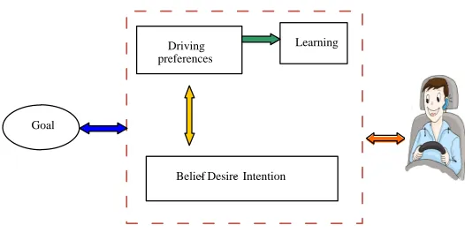
DPL-BDI Agent’s conceptual models are shown as follows in Fig. 3.

Belief- Desire- Intention Driving

preferences

Learning

Goal

Fig. 3.DpL-BDI Agent’s conceptual models

4.1.3. Functional modules

(10)

(1) Multi-attribute decision-making algorithms

To identify theDriving−P ref erencesparametersEiandλi, the LC problems can

be formulated as a constrained nonlinear MADM statement, described as follows:

opt.

min SI min CI

s.t. 

  

  

VM−1(t)

Vm(t)

VM(t)

s(t)

Where, the objective consists of two sub-objectives: minimum the LC safety degree and comfort degree; the constraints consist of four models: speed of the lead vehicle

(VM−1(t)), speed of the lane changer(Vm(t)); speed of the lag vehicle (VM(t)); the

critical lead gap models(t). The parameters to be identified are the weight coefficient

(λi, i = 1,2) of each attribute in this lane-changing MADM problems, as well as, the

unknown parameters in the four constraint models, such as: G, H andτofVmt;β11and

β12ofs(t).

Interactive evolutionary computing (IEC) [16][11] is a kind of evolutionary computing method that the fitness function evaluation needs human to review. In addition, IEC’s other theories and operation parts are as same as the traditional evolutionary computing (such as: Genetic algorithms).Taking advantage of IEC, the procedure towards multi-attribute decision-making algorithms is presented as follows.

Step 1: Initiatet= 0and create an initial population¯atof candidate solutions

randomly over the global searching space;

Step 2: Specify an importance degree for each objective, and, in regard to ev-ery individual, calculate corresponding objective fitness index K based on multi-attribute assessment module;

Step 3: Aided by agents, human operators evaluate the excellent individu-als of candidate solutions in terms of fitness index K. At the same time, agents perform driving behavioral preferences computing and learning algorithms, gen-erating evaluations of individuals for human references;

Step 4: Select excellent individuals based on HCI;

Step 5: Perform crossover and mutation operations to generate the offspring; Step 6: Decode and return to Step 2.

(2) Multi-attribute assessment

Considering a decision-making problem with n attributes, specify an objective fitness index as:

k= n

X

i=1

λiϕi (10)

Where,λi is defined as the relative importance degrees of objectivepithat are

con-strained byPn

i=1λi = 1;ϕiis the achievement degree ofpi. For the proposed methods

in this paper,ϕ1 =

ˆ

SI

SI andϕ2 =

ˆ

CI

(11)

is the realistic safety degree, as well as,CIˆ corresponds to the desired comfort index,CI

corresponds to the realistic comfort index.

(3) Driving behavioral preference learning

The aim of this module is twofold, obtaining human’s driving behavioral preferences and updating the adjustable parameters of preference computing models. Driving behav-ioral preferences’ learning helps agents get access to driver’s preferences towards decision making so as to learn from them, gradually replacing human’s subjective judgment and lessening human’s subjective fatigue and promoting more scientific implementations.

According to the driving behavioral preferences models, interactive learning prob-lems can be formulated as a constrained nonlinear programming statement, described as follows.

min

n

X

m=1

[µ(km)−µ0(km)]2(m= 1, ..., n)

s.t.

P2

i=1λi= 1

τ ₆2 (11)

Where,µ(km),(m = 1, ..., n)corresponds to the Agent’s performance optimal

as-sessment sequences in lane-changing process;µ0(km),(m = 1, ..., n)correspond to the

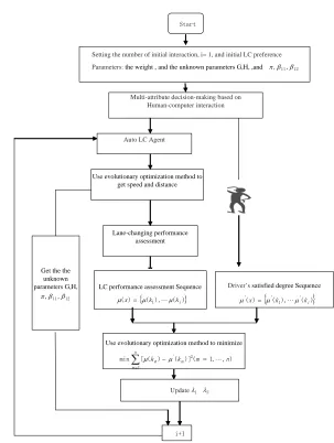
expert driver’s satisfaction degree sequences in LC process. Additionally, genetic algo-rithms can be invoked to solve this optimization problem?whose implementing steps are shown in Fig. 4. A simplified functional structure of the DpL-BDI agents is shown in Fig. 5.

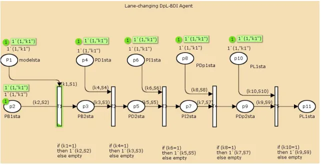
4.2. Agent’s analysis based on Colored Petri nets

Petri nets are used to describe the mathematical model of the parallel and discrete sys-tem, which is suitable for constructing the concurrent and asynchronous computer system model. To study the driving behavioral preference learning algorithm’s rationality and the triggering process, petri nets are employed to realize the components and scheduler of the driving behavioral preferences’ learning (DpL)-BDI agents.

As a kind of high-level Petri net, colored Petri net (CPN) is capable of

descrip-tion and analysis of large and complex Agent’s systems. A well-formed CPN, P

= (C, P, T, A, F, M), is made of six components, where,Cindicates color functions;Pis a

finite set, called place set;T is a finite set, called transition set;Ais a finite set, called arc

set;F ⊆(P×T)∪(T×P)is defined as the flow relationship;M :P → {0,1,2,3, ...}is

defined as the network functions (Marking). In this context, CPNs based DpL-BDI agents could be specified as follows.

Definition 5(Places of agents):

PBis a Belief color set,

PB={PB1 (MADM algorithms),PB2(solutions of MADM)},

PDis a Desire color set,

PD={PD1(multi-attribute fitness index algorithms),PD2(multi- attribute fitness

in-dex values)}.

(12)

Start

Auto LC Agent

Driver’s satisfied degree Sequence

Use evolutionary optimization method to minimize

i+1

Setting the number of initial interaction, i= 1, and initial LC preference Parameters:the weight , and the unknown parameters G,H, ,and

Use evolutionary optimization method to get speed and distance

Update

Multi-attribute decision-making based on Human-computer interaction

Lane-changing performance assessment

Get the the unknown

parameters G,H, LC performance assessment Sequence

12 11,

,  

12 11,

, 

 ₍ ₎



₍ _), '₍ ₎



1 ' '

i

k k x  

  

) , , 1 ( )] ( ) ( [ min

1

2

'_k _m _n

k

n m

m

m   





 

( ), ( )

)

(x k1 ki

  

1

 2

(13)

Intention Set

Learning Set Desire Set Belief Set

LC Decision Making Algorithms

LC Performance assessments

Human-computer interaction Giving human’s preference of lane-changing satisfaction index

Driving preference learning Algorithms

Fig. 5.Functional structure of the DP-L BDI agents

PI = { PI1 (LC assessment index algorithms), PI2(Agent’s assessment index

se-quence)}.

PDpis a driving behavioral preferences’ color set,

PDp ={ PDp1(Human-computer interaction),PDp2( Driver’s satisfied degree index

sequence)}.

PLis a driving behavioral preferences’ learning color set,

PL={PL1( Preferences’ learning algorithms),PL2(updated parametersλ1, λ2)}.

CPN-Tools software is originally developed by the CPN Group at Aarhus University from 2000 to 2010. The tool features incremental syntax checking and code generation, which take place while a Petri net is being constructed. We could in turn build all func-tional modules of agents by CPN metrics. As an exemplary case, the scheduling model for functional modules of agents is presented based on CPN-Tools software in Fig. 6, as well, in which the associated notations are interpreted in Table 1.

5. Case studies

(14)

Table 1.Interpretations of places and transitions associated with the CPN models

Place Color Set Messages Transition Messages

p1 (mode1sta) Model of the Agent’s goal

LC math models ready

T1 Executing the interactive decision making algorithms p2 (PB1sta) State of the first

component in Belief set

Multi-attribute decision-making algorithms ready

T2 Executing the LC performance fitness index computation algorithms p3 (PB2sta) State of the second

component in Belief set

Achievement of a set of evolutionary solutions

T3 Sending the fitness index

p4 (PD1sta) State of the first component in Desire set

LC performance fitness index computation algorithms ready

T4 Interacting

p5 (PD2sta) State of the second component in Desire set

Accomplishment of the

multi-attribute fitness index

T5 Executing the interactive preference learning algorithms p6 (PI1sta) State of the first

component in Intention set

Transferring commands p7 (PI2sta) State of the second

component in Intention set

Agent’s

assessment index sequence ready p8 (PDp1sta) State of the first

component in Driving behavioral preference set

Interaction

p9 (PDp2sta) State of the second component in Driving behavioral preference set

Driver’s satisfied degree index sequence ready p10 (PL1sta) State of the first

component in Learning set

Interactive preference learning algorithms ready p11 (PL1sta) State of the second

component in Learning set

(15)

Fig. 6.Scheduling model for functional modules of agents

5.1. The least squares methods

In the experiments, traffic simulation software Q-Paramics v6.9.3 and VC++6.0 are em-ployed to build the experimental platform in this paper. Paramics was developed for mi-croscopic traffic simulation by the British company Quadstone, as well as, it provided a new-computational tool for the traffic engineers and researchers to understand and analyze the real conditions. Thereafter, a two-way road network model is established, including some constraint such as the road length is 80km, the maximum speed is 120km/h, there’re two intersections on the network.

The total simulation time is defined as 30s; the sampling time is defined as 0.5s. The experimental data consists of vehicle number, road number, the speed of following the vehicle, the forward vehicle number, headway, and the speed of the forward vehicle.

The least square methods are the most commonly traffic trajectory model parameters’ identification method in the LC process [13]. Based on the optimization model and the experimental data (the lane changer is a car, the lead vehicle is a car), Fig. 7 shows the fitting curve of the acceleration in the LC process.

5.2. Traditional GA algorithms

To analyze the LC driving behavioral preference parameters’ difference between different types of vehicles, three common vehicles are selected in this experiment, such as: cars, buses and trucks. Based on the Q-Paramics software, nine LC scenes are performed in this paper, such as: (the lane changer is a car, the lead vehicle is a car; the lane changer is a car, the lead vehicle is a truck; the lane changer is a car, the lead vehicle is a bus; the lane changer is a truck, the lead vehicle is a car; the lane changer is a truck, the lead vehicle is a truck; the lane changer is a truck, the lead vehicle is a bus; the lane changer is a bus, the lead vehicle is a car; the lane changer is a bus, the lead vehicle is a truck; the lane changer is a bus, the lead vehicle is a bus).

(16)

Fig. 7.The fitting curve of the acceleration

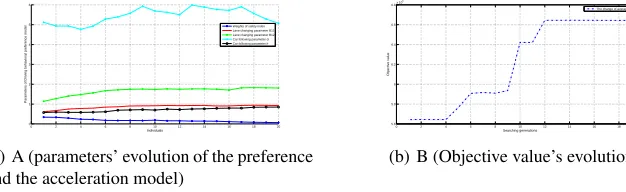
20 generations and 40 individual species to identify the parameters in driving behavior preference LC model. The performances of nine LC scenes are shown in figures 8-16 re-spectively. Fig 17 shows the fitting curve of the acceleration in the LC process (the lane changer is a car, the lead vehicle is a car). In addition, Table 2 presents key data associated with the interaction.

0 2 4 6 8 10 12 14 16 18 20 0

1 2 3 4 5 6 7 8

Individuals

Parameters of Driving behavioral preference model

Weights of safety index Lane changing parameter B11 Lane changing parameter B12 Car following parameter G Car following parameter h

(a) A (parameters’ evolution of the preference and the acceleration model)

0 2 4 6 8 10 12 14 16 18 20 4.6

4.8 5 5.2 5.4 5.6 5.8 6 6.2 6.4 6.6x 106

Searching generations

Objective value

The change of average solutions

(b) B (Objective value’s evolution)

Fig. 8.The profiles of parameters’ evolution (the lane changer is a car, the lead vehicle is a car)

5.3. Using the proposed methods

(17)

0 2 4 6 8 10 12 14 16 18 20 0 1 2 3 4 5 6 Individuals

0 2 4 6 8 10 12 14 16 18 20 0 1 2 3 4 5 6 7x 106

Objective value

The change of solutions The change of average solutions

Fig. 9.The profiles of parameters’ evolution (The lane changer is a car, the lead vehicle is a truck)

0 2 4 6 8 10 12 14 16 18 20 0 1 2 3 4 5 6 7 Individuals

0 2 4 6 8 10 12 14 16 18 20 4

4.5 5 5.5 6 6.5x 106

Objective value

Fig. 10.The profiles of parameters’ evolution (The lane changer is a car, the lead vehicle is a bus)

0 2 4 6 8 10 12 14 16 18 20 0 1 2 3 4 5 6 Individuals

0 2 4 6 8 10 12 14 16 18 20 5.6 5.8 6 6.2 6.4 6.6 6.8x 106

Objective value

Fig. 11.The profiles of parameters’ evolution (The lane changer is a truck, the lead vehicle is a car)

0 2 4 6 8 10 12 14 16 18 20 0 1 2 3 4 5 6 7 Individuals

0 2 4 6 8 10 12 14 16 18 20 4 4.5 5 5.5 6 6.5 7x 106

Objective value

Fig. 12.The profiles of parameters’ evolution (The lane changer is a truck, the lead vehicle is a

(18)

0 2 4 6 8 10 12 14 16 18 20 0 1 2 3 4 5 6 Individuals

0 2 4 6 8 10 12 14 16 18 20 4

4.5 5 5.5 6 6.5x 106

Objective value

Fig. 13.The profiles of parameters’ evolution (The lane changer is a truck, the lead vehicle is a bus)

0 2 4 6 8 10 12 14 16 18 20 0 1 2 3 4 5 6 7 Individuals

0 2 4 6 8 10 12 14 16 18 20 3.5 4 4.5 5 5.5 6 6.5x 106

Objective value

Fig. 14.The profiles of parameters’ evolution (The lane changer is a bus, the lead vehicle is a car)

0 2 4 6 8 10 12 14 16 18 20 0 1 2 3 4 5 6 7 Individuals

0 2 4 6 8 10 12 14 16 18 20 5.2 5.4 5.6 5.8 6 6.2 6.4 6.6 6.8x 106

Objective value

Fig. 15.The profiles of parameters’ evolution (The lane changer is a bus, the lead vehicle is a truck)

0 2 4 6 8 10 12 14 16 18 20 0 1 2 3 4 5 6 7 8 Individuals

0 2 4 6 8 10 12 14 16 18 20 4 4.5 5 5.5 6 6.5 7x 106

Objective value

(19)

Table 2.Key data associated with the interaction

The lane changer The lead vehicle λ1 λ2

Car Car 0.23 0.77

Car Truck 0.25 0.75

Car Bus 0.31 0.69

Truck Car 0.21 0.79

Truck Truck 0.20 0.80

Truck Bus 0.19 0.81

Bus Car 0.18 0.82

Bus Tuck 0.19 0.81

Bus Bus 0.21 0.79

(20)

established, including some constraint such as the road length is 80km, the maximum speed is 120km/h, the minimum critical lag gap is 150m. In this experiment, the lane changer and the lead vehicle are both cars. Speed model of the lead car is defined as

|50×sin(πt)|.

Specify ten generations and eight individual species The performances of initial, third and the last generation are shown in Figures 18, 19 and 20 respectively. In each figure, the first line displays eight speed individuals of the lead car; the second line corresponds to 8 speed individuals of the lane changer, as well as, the third line corresponds to the multi-attribute assessment index(formula (4)). In addition, Table 3 presents key data associated

with the interaction. The expectedSIindex (which isSIˆ in the formula (4)) is described

as 5, as well as, the expectedCIindex (which isCIˆ in the formula (4)) is described as 2.

In the end, using the same experimental data of section 4.1 (the lane changer is a car, the lead vehicle is a car), the fitting curve is shown in Fig. 21.

0 2 4 6 150

160 170 180 190

0 2 4 6 0

2 4 6 8

0 2 4 6 1.5 2 2.5 3 3.5 4

0 2 4 6 150

200 250 300

0 2 4 6 0 1 2 3 4 5

0 2 4 6 1 1.5 2 2.5 3 3.5

0 2 4 6 150

200 250 300 350

0 2 4 6 0 5 10 15 20 25

0 2 4 6 2

4 6 8 10

0 2 4 6 140 160 180 200 220 240

0 2 4 6 0 5 10 15 20 25 30

0 2 4 6 2 3 4 5 6 7 8

0 2 4 6 140 160 180 200 220 240

0 2 4 6 0 0.5 1 1.5 2 2.5 3

0 2 4 6 0

0.5 1 1.5

0 2 4 6 140

160 180 200 220

0 2 4 6 0

5 10 15 20

0 2 4 6 2 3 4 5 6 7

0 2 4 6 140 160 180 200 220 240

0 2 4 6 0 10 20 30 40 50

0 2 4 6 0 5 10 15 20 25

0 2 4 6 150

200 250 300

0 2 4 6 0

10 20 30 40

0 2 4 6 0

5 10 15 Generation: 1 Parents: Offsprings:

Fig. 18.Objectives of the initial population

Table 3.Key data associated with the interaction

Interaction Number λ1 λ2

1 0.235 0.765

2 0.248 0.752

3 0.273 0.727

4 0.296 0.704

5 0.303 0.697

6 0.312 0.688

7 0.335 0.665

8 0.339 0.661

9 0.343 0.657

(21)

0 2 4 6 150

200 250 300

0 2 4 6 0

20 40 60 80

0 2 4 6 0

10 20 30 40

0 2 4 6 140

160 180 200 220

0 2 4 6 0

10 20 30 40

0 2 4 6 2 4 6 8 10 12

0 2 4 6 150

200 250 300

0 2 4 6 0

20 40 60 80

0 2 4 6 2

4 6 8 10

0 2 4 6 150

200 250 300

0 2 4 6 0

20 40 60 80

0 2 4 6 4

5 6 7 8

0 2 4 6 150

200 250 300

0 2 4 6 0

20 40 60 80

0 2 4 6 0

10 20 30 40

0 2 4 6 150

200 250 300

0 2 4 6 0

20 40 60 80

0 2 4 6 0

10 20 30 40

0 2 4 6 150

200 250 300

0 2 4 6 0

20 40 60 80

0 2 4 6 0

5 10 15 20

0 2 4 6 150

200 250 300 350

0 2 4 6 0 10 20 30 40 50

0 2 4 6 4 5 6 7 8 9 Generation: 7 Parents: Offsprings:

Fig. 19.Objectives of the 7th population

0 2 4 6 150

200 250 300

0 2 4 6 0

20 40 60 80

0 2 4 6 0

10 20 30 40

0 2 4 6 150

200 250 300

0 2 4 6 0

20 40 60 80

0 2 4 6 4

5 6 7 8

0 2 4 6 150

200 250 300

0 2 4 6 0

20 40 60 80

0 2 4 6 0

10 20 30 40

0 2 4 6 140 160 180 200 220 240

0 2 4 6 0

20 40 60 80

0 2 4 6 0 5 10 15 20 25 30

0 2 4 6 150

160 170 180 190

0 2 4 6 0

20 40 60 80

0 2 4 6 0

10 20 30 40

0 2 4 6 150

200 250 300

0 2 4 6 0

20 40 60 80

0 2 4 6 2

4 6 8 10

0 2 4 6 100

200 300 400 500

0 2 4 6 0

20 40 60 80

0 2 4 6 4

6 8 10 12

0 2 4 6 140

160 180 200 220

0 2 4 6 0

20 40 60 80

0 2 4 6 0

5 10 15 20 Generation: 10 Parents: Offsprings:

(22)

5.4. Discussion

Based on the three experiments in section 5.1-5.3, we can get the analysis results as fol-lows:

Towards a kind of LC scene, the traditional least squares methods are used to identify the LC model parameters. Because the LC model is nonlinear seriously, the fitting effect of acceleration is not good (Fig. 7).

In order to reflect the different driving behavioral preferences in the different LC scenes, GA is used to get the driving preferences for nine cased based on Q-Paramics. In addition, Fig.17 is compared with Fig.8 to verify that GA is better than the traditional least square methods in fitting the LC process acceleration curve based on the same data in section 5.1.

Finally, we design a kind of LC scene, give the lead car’s velocity equation and set the corresponding LC constraints. Based on the proposed method, we obtain the driving behavioral preferences and the LC model parameters within finite interactions. Fig.21 shows the best fitting effect of LC acceleration based on the same data in section 5.1.

It’s obviously that all the traditional optimization process (the least squares methods and GA) requires historical data which is suffering the flexibility and speediness.

In addition, the proposed driving behavioral preferences’ learning algorithms do not decrease the parameters’ identification accuracy, as well as, they also have the ’online-learning’ characteristics. The complexity of the algorithms does not increase.

6. Conclusions

(23)

BDI models. In contrast to the traditional free LC model, the proposed preferences mod-els are recognized capable of gradually grasping essentials in driver’s subjective judgment in decision-making, as well as helping drivers make decisions more objective and scien-tific. Additionally, colored Petri nets are employed to build driving behavioral preferences (DpL)-BDI agent’ model, as well as, the learning algorithm’s logic is correct based on the CPN-Tools software. The proposed driving behavioral preferences’ learning algorithms do not decrease the parameters’ identification accuracy, as well as, they also have the ’online-learning’ characteristics. To exemplify applications of the approaches, a kind of LC problem is suggested to case studies, giving rise to satisfied results and showing va-lidity of the contribution.

Furthermore, it should be pointed out that this research remains rather fundamental currently, which is in desperate need of further investigations on some key issues, such as: how to record the driver’s preference information, how to design more complex LC model and how to realize the driving behavioral preferences learning algorithms with the wireless vehicle communication equipment in the multi-vehicle environment.

Acknowledgments.This work was supported by the National Natural Science Foundation of China

(No.61273089) ,Beijing Nova Program(No. Z141101001814038) and National Higher-education Institution General Research and Development Project of China (No. 2012JBZ009).

References

1. Adetola, V., Guay, M.: Integration of real-time optimization and model predictive control. Jour-nal of Process Control 20(2), 125–133 (2010)

2. Benedetto, F., Calvi, A., D’Amico, F., Giunta, G.: Applying telecommunications methodology to road safety for rear-end collision avoidance. Transportation Research Part C 50, 150–159 (2015)

3. Casalia, A., Godob, L., Sierrab, C.: A graded bdi agent model to represent and reason about preferences. Artificial Intelligence 175(7-8), 1468 – 1478 (2011)

4. De Souza, G., Odloak, D., Zanin, A.C.: Real time optimization (rto) with model predictive control (mpc). Computers and Chemical Engineering 34(12), 1999 – 2006 (2010)

5. Eason, K.: Ergonomic perspectives on advances in human computer interaction. Ergonomics 34(6), 721 – 741 (1991)

6. Hidas, P.: Modelling lane changing and merging in microscopic traffic simulation. Transporta-tion Research Part C: Emerging Technologies 10(5-6), 351–371 (2002)

7. Jaimes, A., Sebe, N.: Multimodal human-computer interaction: A survey. Computer Vision and Image Understanding 108(1-2), 116 – 134 (2007)

8. Jin, P.J., Yang, D., Ran, B.: Reducing the error accumulation in car-following models calibrated with vehicle trajectory data. IEEE Transacations on Intelligent Transpotation Syetems 15(1), 148–157 (2014)

9. Jin, W.L.: A kinematic wave theory of lane-changing traffic flow. Transportation Research Part B: Methodological 44(8-9), 1001–1021 (2010)

10. Jin, W.L.: A multi-commodity lighthillcwhithamcrichards model of lane-changing traffic flow. Transportation Research Part B: Methodological 57, 361–377 (2013)

11. John, V., Trucco, E., Ivekovic, S.: Markerless human articulated tracking using hierarchical particle swarm optimization. Image and Vision Computing 28(11), 1530–1547 (2010) 12. Kim, I., Kim, T., Sohn, K.: Identifying driver heterogeneity in car-following based on a random

(24)

13. Koriem, S.: Development, analysis and evaluation of performance models for mobile multi-agent networks. computer journal. Computer Journal 49(6), 685–709 (2006)

14. Kyung, G., Nussbaum, M.A.: Driver sitting comfort and discomfort (part ii): Relationships with and prediction from interface pressure. International Journal of Industrial Ergonomics 38(5-6), 526–538 (2008)

15. Kyung, G., Nussbaum, M.A., Babski-Reeves, K.: Driver sitting comfort and discomfort (part i): Use of subjective ratings in discriminating car seats and correspondence among ratings. International Journal of Industrial Ergonomics 38(5-6), 516–525 (2008)

16. Lai, C.C., Chang, C.Y.: A hierarchical evolutionary algorithm for automatic medical image segmentation. Expert Systems with Applications 36(1), 248–259 (2009)

17. Laval, J.A., Leclercq, L.: Microscopic modeling of the relaxation phenomenon using a macro-scopic lane-changing model. Transportation Research Part B: Methodological 42(6), 511–522 (2008)

18. Leclercq, E., Lefebvre, D.: Feasibility of piecewise-constant control sequences for timed con-tinuous petri nets. Automatica 49(12), 3654–3660 (2013)

19. Lu, G., Cheng, B., Lin, Q., Wang, Y.: Quantitative indicator of homeostatic risk perception in car following. Safety Science 50(9), 1898–1905 (2012)

20. Lv, W., Song, W.G., Fang, Z.M., Ma, J.: Modelling of lane-changing behaviour integrating with merging effect before a city road bottleneck. Physica A: Statistical Mechanics and its Applications 392(20), 5143–5153 (2013)

21. Hiemstra-van Mastrigt, S., Kamp, I., van Veen, S., Vink, P., Bosch, T.: The influence of active seating on car passengers’ perceived comfort and activity levels. Applied Ergonomics 47, 211– 219 (2015)

22. McEneaney, J.E.: Agency effects in human-computer interaction. International Journal of Human-Computer Interaction 29(12), 798 – 813 (2013)

23. Mohd Nor, M., Fouladi, M., Nahvi, H., Ariffin, A.: Index for vehicle acoustical comfort inside a passenger car. Applied Acoustics 69(4), 343–53 (2008)

24. Patel, A.M., Joshi, A.Y.: Modeling and analysis of a manufacturing system with deadlocks to generate the reachability tree using petri net system. Ain Shams Engineering Journal 4(4), 831 – 842 (2013)

25. Patire, A.D., Cassidy, M.J.: Lane changing patterns of bane and benefit: Observations of an uphill expressway. Transportation Research Part B: Methodological 45(4), 656–666 (2011) 26. Rahman, M., Chowdhury, M., Xie, Y., He, Y.: Review of microscopic lane-changing models

and future research opportunities. IEEE Transactions on Intelligent Transportation Systems 14(4), 1942–1956 (2013)

27. S., S., Padgham, L.: A bdi agent programming language with failure handling, declarative goals, and planning. Autonomous Agents and Multi-Agent Systems 23(1), 18 – 70 (2011) 28. Sardina, S., Padgham, L.: A bdi agent programming language with failure handling, declarative

goals, and planning. Autonomous Agents and Multi-Agent Systems 23(1), 18–70 (2011) 29. Schubert, R., Schulze, K., Wanielik, G.: Situation assessment for automatic lane-change

ma-neuvers. IEEE Transactions on Intelligent Transportation Systems 11(3), 607 – 616 (2010) 30. Schwarz, C.: On computing time-to-collision for automation scenarios. Transportation

Re-search Part F 27, 283–294 (2014)

31. Tang, T.Q., Wong, S., Huang, H.J., Zhang, P.: Macroscopic modeling of lane-changing for two-lane traffic flow. Journal of Advanced Transportation 43(3), 245–273 (2009)

32. Tideman, M., van der Voort, M.C., van Arem, B.: A new scenario based approach for designing driver support systems applied to the design of a lane change support system. Transportation Research Part C: Emerging Technologies 18(2), 247 – 258 (2010)

33. Valencia-Garcia, R., Garcia-Sanchez, F.: Natural language processing and humanccomputer interaction. International Journal of Human-Computer Interaction 35(12), 415 – 416 (2013) 34. Wu, L., Su, K., Sattar, A., Chen, Q., Su, J., Wu, W.: A complete first-order temporal bdi logic

(25)

35. Wu, L., Su, K., Sattar, A., Chen, Q., Su, J., Wu, W.: A complete first-order temporal bdi logic for forest multi-agent systems. Knowledge-Based Systems 27, 343–51 (2012)

36. Yeung, J.S., Wong, Y.D.: The effect of road tunnel environment on car following behaviour. Accident Analysis and Prevention 70, 100–109 (2014)

37. Yu, P., Hua-Yan, S., Hua-Pu, L.: Analysis of phase transition in traffic flow based on a new model of driving decision. communications in theoretical physics. Communications in Theo-retical Physics 56(1), 177 – 183 (2011)

38. Zheng, J., Suzuki, K., Fujita, M.: Predicting drivers lane-changing decisions using a neural network model. Simulation Modelling Practice and Theory 42, 73–83 (2014)

39. Zheng, Z.: Recent developments and research needs in modeling lane changing. Transportation Research Part B: Methodological 60, 16–32 (2014)

40. Zheng, Z., Ahn, S., Chen, D., Laval, J.: The effects of lane-changing on the immediate follower: Anticipation, relaxation, and change in driver characteristics. Transportation Research Part C: Emerging Technologies 26, 367 – 379 (2013)

Jian Wangreceived the B.S, M.S and Ph.D. degrees for Beijing Jiaotong University, Bei-jing, China, in 2000, 2003 and 2007 respectively. He was a lecturer with the School of Electronic and Information Engineering, Beijing Jiaotong University from 2007 to 2010. Currently, he is an Associate Professor with Beijing Jiaotong University. His professional interests include Intelligent Transportation System, train control system, new GNSS ap-plications in railway.

BaiGen Caireceived his B.S., M.S., and Ph.D. degree in Traffic Information Engineering and Control from Beijing Jiaotong University in 1987, 1990, and 2010 respectively. Since 1990 he has been on the faculty at School of Electronic and Information Engineering in Beijing Jiaotong University. He was a visiting scholar to Ohio State University from 1998 to 1999, and currently he is a Professor and the chief of Science and Technology Division of Beijing Jiaotong University. His research interests include train control system, Intelli-gent Transportation System, GNSS navigation, multi-sensor fusion, and intelliIntelli-gent traffic control.

Jiang Liureceived his B.S. degree and Ph.D. degree in Intelligent Transportation Engi-neering from Beijing Jiaotong University in 2007 and 2011 respectively. He was a post-doctor at School of Transportation Science and Engineering in Beihang University from 2011 to 2013. He is currently an Associate Professor at School of Electronic and Infor-mation Engineering, Beijing Jiaotong University. His research interests include satellite navigation, intelligent transportation system, nonlinear estimation, and geographic infor-mation system.

(26)

Modeling, simulation and Testing, GNSS (GPS, Galileo, Glonass and BDS)/GIS, Inte-grated Navigation, Intelligent Transportation System, Cooperative Vehicle Infrastructure System of China (CVIS-C).