Dimension Reduction and Classification of Hyperspectral Images based on Neural Network Sensitivity Analysis and Multi-instance Learning

Dimension Reduction and Classification of

Hyperspectral Images based on Neural Network

Sensitivity Analysis and Multi-instance Learning

Hui Liu1,2_{, Chenming Li}1 _{and Lizhong Xu}1

1 College of Computer and Information Engineering, Hohai University, Nanjing, 211100, China, [email protected]

2 School of Science, Jiangxi University of Science and Technology, Ganzhou, 341000, China, [email protected]

1 College of Computer and Information Engineering, Hohai University, Nanjing, 211100, China, [email protected]

Abstract. Hyperspectral remote image sensing is a rapidly developing integrated technology used widely in numerous areas. The rich spectral information from hyperspectral images aids in recognition and classification of many types of objects, but the high dimensionality of these images leads to information redundancy. In this paper, we used sensitivity analysis for dimension reduction. However, another challenge is that hyperspectral images identify objects as either a "different body with the same spectrum" or "same body with a different spectrum." Therefore, it is difficult to maintain the correct correspondence between ground objects and samples, which hinders classification of the images. This issue can be addressed using multi-instance learning for classification. In our proposed method, we combined neural network sensitivity analysis with a multi-instance learning algorithm based on a support vector machine to achieve dimension reduction and accurate classification for hyperspectral images. Experimental results demonstrated that our method provided strong overall classification effectiveness when compared with prior methods.

Keywords: Sensitivity Analysis, Artificial Neural Network, Ruck Sensitivity Analysis, Dimension Reduction, Classification, Hyperspectral Images, Multi-instance Learning, SVM

1.

Introduction

between ground objects and samples, which makes classification of the images difficult and computationally costly. This issue can be addressed using multi-instance learning for classification. In this research, we combine neural network sensitivity analysis with a multi-instance learning algorithm based on a support vector machine (SVM) to achieve dimension reduction for hyperspectral remote sensing images.

Hyperspectral imaging differs from general multispectral imaging insofar as hyperspectral imaging can display two-dimensional spatial information for a region of interest (e.g., the earth's surface), and it can add a dimension of spectral information. Multispectral images include only a few spectral bands, whereas hyperspectral images include hundreds of bands that are much narrower. Therefore, hyperspectral images can form an "image cube" [1]. In addition to multiple bands, hyperspectral images have distinct characteristics such as large amounts of data and high information redundancy that present difficulties for storing, transmitting, and processing the images. As a result, a band selection operation must be performed to reduce some of the unnecessary bands before processing hyperspectral images [2]. This operation helps to decrease the calculation requirements for hyperspectral image classification, and effectively avoids the Hughes phenomenon [3].

Hyperspectral image band selection can be considered an NP-hard combinatorial optimization problem [4]. Typically, search algorithms are used to search a band subset, allowing the evaluation standard to achieve its optimal value across all of the bands of the hyperspectral image. This queried band subset can then be treated as the optimal band combination. The common method of band selection and dimension reduction [5] for hyperspectral remote sensing images is to select several bands from the whole band to represent the whole band space. This approach requires that the band combination selected be able to provide effective improvement for classification accuracy in the subsequent classification. For this research, we select the band according to the band’s contribution to classification. Bands that help to improve classification accuracy are selected first.

For classification of hyperspectral remote sensing images, neural network classifiers are commonly used because they work well for classifying images with high dimensionality and nonlinear structures. To provide a quantitative evaluation of the effects of one band on classification accuracy, a neural network sensitivity analysis can be employed that is based on a neural network classifier. Sensitivity analysis by a neural network [6] can provide a quantitative description of the influence of the input variables of a model on the output variables. The sensitivity coefficient of the model properties is sorted. Properties with larger sensitivity coefficients are chosen, and those with smaller ones are no longer included. In this way, the model is simplified, and the complexity of model processing is reduced. In this paper, we apply neural network sensitivity analysis to the band selection for hyperspectral remote sensing images, combined with a frequently used BP neural network classifier.

Analysis and Multi-instance Learning 445 several “bags” labeled with concept tags. Each bag contains several instances without concept notations. A bag is labeled positive if it contains at least one instance that is positive, and a bag is labeled negative if all of the instances in it are negative. By learning from the training bags, the learning system can predict the concept tag of a bag that is outside the training set as correctly as possible. Following on the work of T. G. Dietterich et al., many researchers began to devise practical multi-instance learning algorithms. Multi-instance learning stirred great interest in the machine learning field because it was a promising new learning framework in an area of machine learning previously unexplored. Multi-instance learning has unique properties and continues to offer good prospects for wide application.

A pixel-level classifier can help to divide the remotely sensed hyperspectral imagery, but if spectral background noise and clutter noise are present, classification accuracy will be decreased because of omissions or faults. Recently, some researchers proposed to adopt classification based on pattern spot images to solve the omissions or faults brought by spectrum changes. A pattern spot image refers to the single zone whose shape shares the same features with a spectrum. CHEN Jie et al. [8] put forward the rough set theory-based object-oriented classification of high resolution remotely sensed imagery. First, they abstracted the pattern spot image by means of watershed segmentation. Next, they analyzed the texture features of the abstracted images using Gabor wavelets, and divided the texture classification rules for abstracted images based on rough set theory. ZHANG Chuan et al. put forward object-oriented classification of high resolution remotely sensed imagery [9]. YANG Chang-bao et al. explored the object-oriented classification of remotely sensed imagery, and they determined the classification by segmenting the orthorectification SPOT image based on a distributed domain solver [10]. TAN Yu-min et al. put forward an object-oriented remote sensing image segmentation approach based on edge detection. [11]. Pattern spot image classification differs greatly from pixel-based classification because the former includes various regional texture space information, while the latter has only spectral features. Pixel-based classification considers only the features of a single pixel. Classification based on pattern spot images is less likely to be disturbed by spectral background noise and is more likely to retain regional integrity since it is abstracted by the regional spectra and space characteristics.

However, pattern spot image classification still has weaknesses in terms of its anti-noise properties that result in low classification accuracy with accompanying omissions or faults. Since the anti-noise property fails to provide the needed filtering, the classification will be less likely to be disturbed by noise with simulti-instance learningar spectra and space characteristics classified in the same zone, which is bigger than the object by making use of the regional relevance and object-oriented basis. DU Pei-jun et al. proposed that the cases in which different objects may have the same spectra characteristics or the same object may have different spectra characteristics, together with the noise in training instances, can be regarded as particular representatives of “ambiguity” in the training bag multi-instance learning. Therefore, when objects from the image segmentation are regarded as an instance in multi-instance learning, the object set of clutter is regarded as the bag, and multi-instance learning can be used in remote sensing classification [12].

remote sensing images. The complexity of land surface composition and the difficulty in selecting training samples cause the classification process to be highly dependent on human experience and prior knowledge. When using sensitivity analysis provided by an artificial neural network to realize dimension reduction for hyperspectral images, all of the bands are divided into several groups, as long as a lower correlation exists between adjacent bands. In addition, a differential evolution (DE) algorithm is used for optimizing the neural network structure. The bands that make only small contributions are given up based on the Ruck sensitivity analysis method.

Given the special advantages of multi-instance learning for solving ambiguous problems, and the advantages of neural network sensitivity analysis for dimension reduction, we suggest that integrating both multi-instance learning and sensitivity analysis for hyperspectral image classification can reduce the uncertainty of classification results. In view of this background and the benefits of applying new machine learning methods to remote sensing image classification, in this paper, we combine multiple-instance learning and an ensemble artificial neural network with embedded sensitivity analysis to improve the accuracy of hyperspectral image classification.

2.

Related Work

2.1. Neural Network Sensitivity Analysis

Sensitivity analysis is an important research focus in the field of neural networks. In some practical applications, the availability of a huge amount of data can cause the trained neural network to become increasingly complex. The main task of sensitivity analysis is to determine how to analyze the parameters of the neural network effectively and simplify the scale of the network. Toward this end, we use the following procedure in this research.

Assume that the model is y= f x x

(

)

sensitivity coefficient of property xi _{on output value}y_{: the higher the sensitivity} coefficient, the greater the influence of the property on the output value. Thus, the sensitivity analysis can provide a quantitative description of the influence of the input variables on the output variable of a model. Furthermore, we can sort the sensitivity coefficients of the model’s properties. We can choose the properties with larger sensitivities and give up the smaller ones according to the practical considerations of the problems. In this way, the model can be simplified and the computational complexity of processing the model reduced, which means dimension reduction is achieved.

Analysis and Multi-instance Learning 447 mechanisms of the data work. In such cases, they cannot build the model expression

( )

y=f x

directly, and therefore cannot conduct a sensitivity analysis either. However, researchers have shown that while a neural network does not need to model the physical concept of the research question, the neural network can provide more effective solutions for problems involving uncertainty or nonlinearity. The network provides a black box analysis model, and outputs reasonable results through the training and learning of input samples [14]. If the input data and output data are known, the neural network will use many simple neurons to simulate the non-linear relationships between the data. Neural network sensitivity analysis also uses the connection weights and the threshold between neurons to assess the influence of the input data on the output data [15].

Neural network sensitivity analysis can be divided into local sensitivity analysis and global sensitivity analysis. Some scholars have focused mainly on the study of local sensitivity analysis. There are four types of classical neural network sensitivity analysis. The first type is the sensitivity analysis method based on the connection weight, such as the Garson algorithm put forward in the early 1990s by Garson [16] and the Tchaban algorithm proposed by Tchaban [17]. The second type is sensitivity analysis based on the influence of the partial derivatives of output variables on input variables, such as Dimoponlos sensitivity analysis [18] and Ruck sensitivity analysis [19]. The third type is sensitivity analysis combined with statistics, such as methods based on random testing by Olden et al.[20]. The forth type is sensitivity analysis based on input variable disturbance, such as the method of adding white noise to the input data of a network and calculating the resulting change of output variables, an example of which was put forward by Scardi [21]

2.2. SVM Classification Methods and Multi-instance Learning

Training data are required to train the SVM model. However, these data cannot be separated without errors. The data points that are closest to the hyperplane are used to measure the margin, while the SVM attempts to identify the hyperplane that maximizes the margin and minimizes a quantitative proportion to the number of misclassification errors [22]. The SVM derives the optimal hyperplane as the solution of the following convex quadratic programming problem [23]:

(

)

, , 1

1

. . 1 , 0, 1, 2, , 2

min

n

T T

i i i i i

w b i

w w C s t y w x b i n

 =   

+



, (1)

where {( , ),x y1 1 ,( , )}x yi i _{are the labeled training datasets with} d i

xR _and

 

y −

; w* and b* define a linear classifier in the feature space; C is the regularization parameter defined by the user; and i _{is a positive slack variable that} handles permitted errors.

1 1 1 1

1

max ( ) ( , ), 0 , 1,2 . . 0

2

n n n n

i i j i j i j i i i

i i j i

Q   x x K x x  C i n s t x

= = = =

=







, (2)

where   =[ ,1 2, ,n] _{is the vector of the Lagrange multipliers, while} K( , ) _{is a} kernel function. For a linearly non-separable case, a kernel function is introduced that satisfies the condition stated by Mercer’s theorem and that corresponds to some types of inner product in the transformed (higher) dimensional feature space, as shown:

( ,i j) ( )i ( )j

K x x = x  x

. (3)

The final result is a discrimination function F x( ) conveniently expressed as a function of the data in the original (lower) dimensional feature space:

* * * *

1

( ) sgn[( ) ( ) ] sgn( ( , ) )

n T

i i i i

F x w  x b  y K x x b

=

= + =



. (4) Some popular kernel functions include the following: a) Linear kernel

( , )_i ( _i)

K x x = x x _{, (5)}

Polynomial kernel ( , ) [( T ) 1]q

i i

K x x = x x + _{, (6)}

where q is a constant.

b) Gaussian Radial Basis Function kernel

,

2 2

( , )i exp i , 0

x x

K x x 



 ₋ 

 

= −  

 

  _{, (7)}

Sigmoid kernel

( , ) tanh[ ( T ) ], 0, 0

i i

k x x = v x x +c v c _{. (8)}

Analysis and Multi-instance Learning 449 Traditional supervised learning can be treated as a special case of multi-instance learning. The transformation of traditional supervised learning algorithms to make them capable of dealing with multiple instance problems is an important branch in multi-instance learning algorithm research. Considering the bag concept, multi-multi-instance learning can be viewed as a generalization of traditional supervised learning. Combining multiple learners for the purpose of enhancing the performance of the base learner is an effective method in traditional supervised learning frameworks. According to the supervised nature and classification function of multi-instance learning, multiple instance ensemble learning is also a feasible approach, and some researchers have shown that performance is increased by using an ensemble. Research into the integration of ensemble learning and multi-instance learning is an active branch of machine learning, so advances have been seen in remote sensing image classification (Qi, et al., 2011; Zhou, et al., 2003; Auer & Ortner, 2004; Kittler, et al., 1998).

Multi-instance learning algorithms based on an SVM can be divided into two categories: multi-instance learning based on samples (mi-SVM), and multi-instance learning based on bags (MI-SVM) [27–28]. mi-SVM tries to identify a maximal margin hyperplane for the instances, subject to the constraint that at least one instance of each positive bag is located in the positive half-space while all instances of negative bags are in the negative half-space. MI-SVM tries to identify a maximal margin hyperplane for the bags by regarding the margin of the “most positive instance” in a bag as the margin of that bag.

(

)

 

2 { }

1

: min min , . . : , 1 , 0, 1,1

2

i

i i i i i i

y

i

mi−SVM w +C



1

1, . . 1, 1, . . 1

2 i

I i I

i I

y

I s t Y and y I s t Y

 + _{  = = −  = −}



(

)

: min , . . : max , 1 , 0

2 i i i I I

w b i I

I

MI SVM w C s t I Y w x b

    

− +



, (10)

where w and b are two parameters; i_{is a positive slack variable;} xi_{is the input value;}

 

y −

is the output value; and C is the regularization parameter defined by the user.

3.

Application of Neural Network Sensitivity Analysis and

Multi-instance Learning to Band Selection

network. Last, the optimized BP neural network is used to conduct the sensitivity analysis. The sensitivity analysis results for all of the test samples are combined by using the comprehensive evaluation function, and finally the band with the biggest influence on classification results is selected. The specific process is explained in the following subsections of this paper.

3.1. Data Preprocessing and Band Selection

For the proposed method, data processing takes place using the following steps. Before employing the neural network sensitivity analysis, the original hyperspectral remote sensing image needs to be preprocessed to eliminate the bands that have interference from noise, water vapor, or other serious pollution. Select the object that has the largest number of samples as the pre-selected object that is good for classification. Typically, the original hyperspectral remote sensing image has a large number of bands, but there is a high correlation and high redundancy between bands. Therefore, to attain a good result from the sensitivity analysis, it is very important to choose as the input the band that also has a weak correlation.

To solve the above problem, the approach is to divide the whole band into several subspaces, and then select the band. The adaptive subspace decomposition (ASD) [30] method based on correlation filtering is used to divide the band set of the hyperspectral

remote sensing image. First, we calculate the correlation coefficient denoted as Rij

between the two bands. Let ui _and uj _{denote the number of i and j bands, respectively.} As the value of the correlation coefficient grows larger, the correlation between bands becomes stronger, and as the correlation comes closer to 0, the correlation becomes

weaker. Rij _{is defined as:}

(

)(

)





(

)







(

)



,

2 2

i i i i i j

i i j j

E x x R

E x E x

 

 

− −

=

− −

. (11)

The value Rij _{of the matrix R ranges between 0 and 1. As Rij comes closer to 1, the}

correlation between the two bands becomes stronger. i _and j _{are the mean values of}

i

x _and xj_{, respectively. They denote the gray mean values of the two bands.} E[ ]• _{is the}

mathematical value expected. When all Rij _{values are identified, then the proper}

threshold Tb _{is set. The continuous bands of} |Rij|Tb _{form a new subspace. We can} control the number of subspaces and the number of bands in each subspace dynamically

Analysis and Multi-instance Learning 451 input, and expected value T_Test for output, all of which are required for the training of a BP neural network. These steps make it convenient to determine the topological structure of the neural network.

3.2. Dimension Reduction and Classification based on Sensitivity Analysis and

Multi-instance Learning

3.2.1 Ruck sensitivity analysis

Ruck sensitivity analysis (1990) is based on the partial derivatives of output variables for input variables. This method is designed for feedback neural networks, such as BP neural networks and RBF neural networks. This approach, which is simple and fast, evaluates the partial derivatives with the activation function of the neural network, and calculates the influence of the input data on the output data. Therefore, Ruck sensitivity analysis is used to study band selection for a hyperspectral remote sensing image based on a BP neural network classifier.

The value Rij _{of the matrix R ranges between 0 and 1. As Rij comes closer to 1, the}

correlation between the two bands becomes stronger. i _and j _{are the mean values of}

i

x _and xj_{, respectively. They denote the gray mean values of the two bands.} E[ ]• _{is the}

mathematical value expected. When all Rij _{values are identified, then the proper}

threshold Tb _{is set. The continuous bands of} |Rij|Tb _{form a new subspace. We can} control the number of subspaces and the number of bands in each subspace dynamically

by changing the threshold Tb_{. Furthermore, Rs denotes the ratio of the number of bands} in a subspace to the total number of bands in all subspaces. We select the bands in each subspace to create band combinations according to the ratio Rs. Then we reduce the correlation of the bands as much as possible. Combining the bands with the pre-object types and the object information of the original remote sensing image, we can determine the training sample P for input, expected value T for output, test sample P_Test for input, and expected value T_Test for output, all of which are required for the training of a BP neural network. These steps make it convenient to determine the topological structure of the neural network.

The above Ruck sensitivity analysis is used only for the sensitivity analysis of the input value to the output value of a single sample test point. A comprehensive evaluation function is needed to synthesize the sensitivity analysis results of each single sample point. Here, we apply the MSA metrics proposed by Jacek. M [25] is chosen as the synthetic evaluation function. Assume Sik _{denotes the sensitivity coefficient of the input}

variable i of all the samples to the output variable Y kk

(

)

( )

n t ik t ik

s S

n

= =



, (15)

where n denotes the total number of samples, and Sik _{is nonnegative.} Sik _{can be used} to sort the sensitivity of the input bands, and then the influence of the input variable to the output results can be measured.

3.2.2 Band Classification Using Neural Network Sensitivity

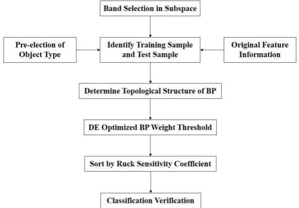
First, according to the proportion Rs in each subspace, several bands are selected to form a band combination. Combined with the pre-selected object type, the training sample P and the test sample P_Test are generated, which then serve as the input variables of the BP neural network. The number of band combinations is equal to the number of the neurons at the input end. Furthermore, the label value of the ground object type is used as the output of the BP neural network. Then, the training samples (with results T) and test samples (with results T_Test) are generated. In addition, the weight and threshold of the BP neural network are optimized by a DE algorithm. All of the samples are classified by the optimized BP neural network, and the results of the sensitivity analysis are calculated. In addition, bands are sorted according to their sensitivity coefficients. Bands with smaller sensitivity coefficients will be given up, and bands with important effects on classification results will be identified. Last, the screened band combinations are classified using the neural network classifier to verify the effect of dimension reduction. The flow of the procedure is shown in Figure 1.

Analysis and Multi-instance Learning 453

3.2.3 Classification of Hyperspectral Remote Sensing Image based on Multi-instance Learning

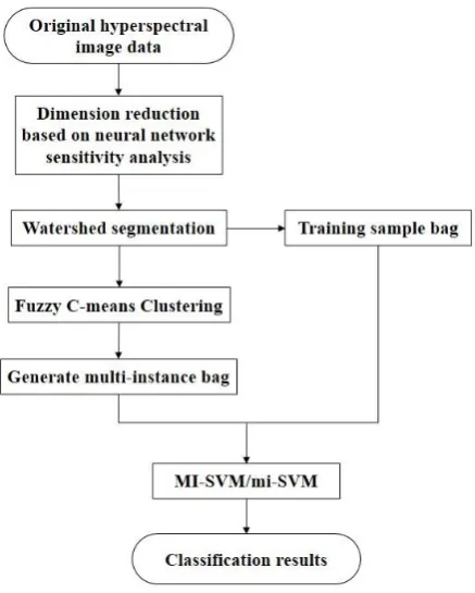
As described above, in multi-instance learning [31–32], the training set is composed of labeled bags, and the bags are made up of non-labeled samples. The goal of multi-instance learning is to predict the label of previously unseen bags by learning the training set. Classification by bags as a unit includes many more features than classification by pixels or by the object as a unit, and both the anti-noise capability of the region and the accuracy of classification are improved. Each feature of the segmented object is taken as an instance; the object set generated by the clustering is taken as the packet. Using the packets, multi-instance learning based on an SVM is used for classification. In this paper, first, based on the dimension reduction of the band, the watershed transform algorithm is utilized to decompose the image into several objects that are used as instances for multi-instance learning. Then, the training samples are constructed with instances selected by artificial selection, and the unknown bags are obtained by the clustering algorithm. The new bag is marked with the nearest sample category that has maximum diversity. In other words, the number of generated bags is completely determined by the clustering algorithm. The steps of the algorithm are as follows.

(1) Reduce the dimension of the hyperspectral band by using neural network sensitivity analysis.

(2) Obtain the object by applying the common watershed algorithm.

(3) For each band that is selected by the band selection method, calculate the property of the object, and construct the property space.

(4) Multi-instance bags are generated by the fuzzy C-means clustering

(5) Select samples for each kind of object to form a training sample bag, and use an SVM for classification.

(6) Get the classification results.

The flow of the classification process is shown Figure 2.

4.

Experiments and Results

4.1. Design of the Experiment

We designed some simulation experiments to demonstrate empirically the effectiveness of our proposed method for dimension reduction of hyperspectral remote sensing images using neural network sensitivity analysis and multi-instance learning. The experimental program was developed using MATLAB R2009b. The SVM classifier utilized the LIBSVM toolkit (http://www.csie.ntu.edu.tw/~cjlin/libsvm/) and adopted a radial basis function (RBF) to perform the experiments. The penalty factor of the SVM was 16. The BP neural network was realized by the built-in neural network toolbox of MATLAB. We designed the experiment using a standard hyperspectral image. The dataset was revised in MAT format, which can be obtained from the website http://www.ehu.eus/ccwintco/index.php?title=Hyperspectral_Remote_Sensing_Scens. The image was part of a hyperspectral image from a mixed agroforestry experimental zone in northwestern Indiana (USA). It was acquired by the AVIRIS sensors in June 1992. In this image, the range of wavelengths was 0.4~2.5 um, the size of image was 145*145 pixels, and the spatial resolution of the image was 25m. In the pretreatment of the original image [24] (including image denoising and image deblurring), the bands that were heavily polluted by water vapor and noise (such as bands 1~4, 78, 80~86, 103~110, 149~165, and 217~224) were removed from the original bands. The remaining 179 bands were kept for experimental purposes. Figure 3 is an RGB false color image composite of the selected bands: 50, 27, and 17. Figure 4 is the real distribution image of the 7 objects chosen for the experiments.

Analysis and Multi-instance Learning 455

Fig. 3. The AVIRIS false color image

Fig. 4. The real distribution image

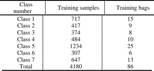
Table1. Training samples and test samples

Class

number Training samples Training bags

Class 1 717 15

Class 2 417 9

Class 3 374 8

Class 4 484 10

Class 5 1234 25

Class 6 307 6

Class 7 647 13

4.2. Results and Analysis

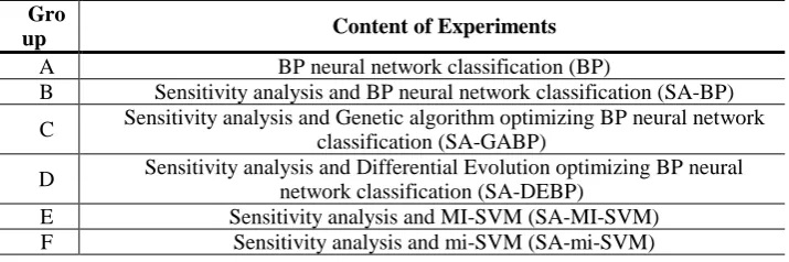
A DE algorithm was used to optimize the BP neural network to get better results from the sensitivity analysis, which meant the band combination could improve the accuracy of classification effectively after the band with the smallest sensitivity coefficient was eliminated. Furthermore, to some extent, the multi-instance learning method based on the SVM could improve classification accuracy. We designed six experiments to demonstrate the superiority of the multi-instance learning method based on an SVM and optimizing the BP neural network with the DE algorithm. The band combinations used in the experiments were the same ones selected under the same subspace division. The detailed content of the experiments is shown in Table 2.

Table 2. Comparison experiments

Gro

up Content of Experiments

A BP neural network classification (BP)

B Sensitivity analysis and BP neural network classification (SA-BP)

C Sensitivity analysis and Genetic algorithm optimizing BP neural network classification (SA-GABP)

D Sensitivity analysis and Differential Evolution optimizing BP neural network classification (SA-DEBP)

E Sensitivity analysis and MI-SVM (SA-MI-SVM)

F Sensitivity analysis and mi-SVM (SA-mi-SVM)

In each experiment, six types of bands with different numbers were compared, and the values of

Rs were selected relatively as 1/9, 1/6, 2/9, which meant selecting the band whose number was about 20, 30, or 40 from the divided subspace in accordance with the proportion of Rs. The topology structure of the BP neural network was set as the N number of neurons of the input layer equal to the number of bands in each group. The number of the types of primary features was 7, which was also the total number of the classification. The number of the neurons of output layer

M was set as 7. The hidden layer was set to be single, and the number of its neurons L was set

according to the expression L= N+M+a. In this expression, a is the adjustment constant between 1 and 10. L changed with the training sample set, and ultimately it was determined that the error of the network was minimal when a = 5. The related parameters of the BP neural network training and DE algorithm were set as shown in Table 3 and Table 4.

Table 3. The setting of the parameters of BP

BP Parameters Parameters setting

Frequency of training 1000

Minimum mean square error 0.01

Learning rate 0.1

Hidden layer activation

Analysis and Multi-instance Learning 457 Output layer activation

function Linear function purelin

Training function Levenberg-Marquadt Back propagation algorithm

Table 4. The setting of the parameters of DE

Parameters Parameter values

Individual dimension D D = N*L+L+L*M+M

Population size Nd Nd = 20

Population size MAXGEN MAXGEN = 50

Hybridization parameters CR CR = 0.9

Differential evolution model DE/best/1/bin

Except for group A, the other five groups of experiments needed to calculate the sensitivity coefficient. Considering the large number of sensitivity coefficients, Tables 5–7 show only the sensitivity coefficients of three kinds of bands. In the experiments with group D, these bands were analyzed using the Ruck method. In the table, the sensitivity coefficients are arranged in order from largest to smallest.

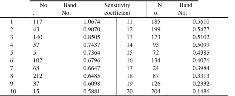
Table 5. Sensitivity coefficient of 20 Bands

No .

Band No.

Sensitivity coefficient

N o.

Band No.

1 117 1.0674 11 185 0.5610

2 43 0.9070 12 199 0.5477

3 140 0.8505 13 173 0.5102

4 57 0.7437 14 93 0.5099

5 5 0.7364 15 72 0.4385

6 102 0.6796 16 134 0.4076

7 68 0.6647 17 24 0.3984

8 212 0.6485 18 87 0.3313

9 37 0.6098 19 126 0.2332

10 15 0.5881 20 204 0.1486

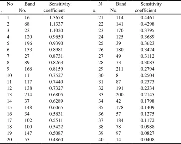
Table 6. Sensitivity coefficient of 30 Bands

No .

Band No.

Sensitivity coefficient

N o.

Band No.

Sensitivity coefficient

1 16 1.2224 16 141 0.3852

2 114 0.8933 17 73 0.3778

3 178 0.8743 18 37 0.3076

4 34 0.8259 19 87 0.3013

6 133 0.7176 21 148 0.2474

7 97 0.7028 22 191 0.1856

8 100 0.6639 23 200 0.1725

9 89 0.6369 24 170 0.1615

10 211 0.6300 25 8 0.1520

11 39 0.6259 26 42 0.1117

12 13 14 15 125 27 196 184 0.5951 0.5242 0.4252 0.3990 27 28 29 30 11 57 68 166 0.0909 0.0867 0.0814 0.0596

Table 7. Sensitivity coefficient of 40 Bands

No . Band No. Sensitivity coefficient N o. Band No. Sensitivity coefficient

1 16 1.3678 21 114 0.4461

2 68 1.1337 22 141 0.4298

3 23 1.1020 23 170 0.3795

4 120 0.9650 24 125 0.3689

5 196 0.9390 25 39 0.3623

6 133 0.8981 26 180 0.3424

7 27 0.8731 27 49 0.3112

8 89 0.8263 28 73 0.3083

9 166 0.8159 29 211 0.2794

10 11 0.7527 30 8 0.2504

11 117 0.7440 31 87 0.2373

12 138 0.7327 32 191 0.2334

13 214 0.6805 33 200 0.2145

14 37 0.6289 34 42 0.1798

15 148 0.6065 35 178 0.1409

16 34 0.5631 36 57 0.1275

17 102 0.5511 37 184 0.1172

18 100 0.5422 38 78 0.0988

19 147 0.5087 39 97 0.0827

20 53 0.4860 40 14 0.0408

Analysis and Multi-instance Learning 459

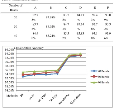
Table 8. Classification accuracy

Number of

Bands A B C D E F

20 82.7

5% 83.68%

83.7

5%

84.13

%

92.4

3%

93.0

9%

30 83.7

5% 84.02%

84.7

3%

85.14

%

92.7

8%

93.3

2%

40 84.9

0% 85.24%

85.5

2%

85.83

%

93.1

8%

93.9

6%

Fig. 5. Classification accuracy curves

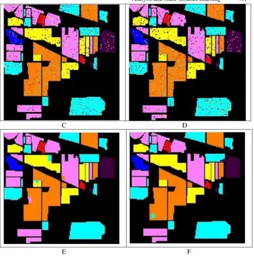
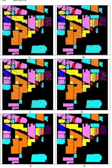
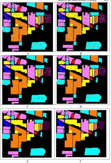
For classification, groups E and F used sensitivity analysis combined with multi-instance learning based on samples (mi-SVM) and multi-multi-instance learning based on bags (MI-SVM), respectively. With the same number of bands, the classification accuracy of groups E and F was significantly higher than for groups B, C, and D, at more than 90%. These results demonstrate that in terms of classification, multi-instance learning performed better than the BP neural network. In addition, using multi-instance learning not only improved the classification accuracy, but also achieved an ideal classification effect. The classification accuracy using 30 bands was higher than when using 20 bands, and the classification accuracy using 40 bands was higher than when using 30 bands. This result indicates that with an increase in the number of bands, the classification accuracy of the same group improved. With the increased number of bands, the classification accuracy of groups E and F was more than 90%, which means that sensitivity analysis and multi-instance learning are very suitable for the classification of hyperspectral image. Figures 6–8 show the results of six groups of experiments using 20, 30, and 40 bands. It can be seen directly from these figures that groups A and B had the fewest incorrect classifications and higher classification accuracy regardless of the number of bands.

Finally, we compared the classification performance of the proposed method with some other hyperspectral image classification methods, as shown in Table 9. In this table, the accuracies outside the brackets were taken from corresponding references directly, and those accuracies in the brackets were obtained by our proposed method. All of the methods were tested under the same conditions with 7 classes and 5% trainings samples. Table 9 demonstrates that the classification performance of the proposed method outperformed all of the compared methods.

Analysis and Multi-instance Learning 461

C D

E F

A B

C D

E F

Analysis and Multi-instance Learning 463

A B

C D

E F

Table 9. Comparison with other methods

References Baseline Feature Overall

Accuracy

Sun et al. [33] RWASL Spectral 94.15%

Guo et al. [34] FSAF Spectral 84.36%

Li et al. [35] KELM Spectral 84.53%

Hu et al. [36] RBF-SVM Spectral 90.74%

Proposed

method

SA-MI-SVM Spectral 94.21%

Proposed

method SA-mi-SVM Spectral 94.28%

5.

Conclusions

Hyperspectral images take objects as the basic classification unit in a manner similar to the examples and packages used in multi-instance learning. Therefore, multi-instance learning can be used for the classification of remote sensing images. In this research, we combined neural network sensitivity analysis with a multi-instance learning algorithm based on an SVM to achieve dimension reduction and classification of hyperspectral remote sensing images. First, to reduce the correlation among the input properties, we used adaptive subspace division to select band combinations. In addition, a DE algorithm was adopted to optimize the BP neural network. To provide stable network connection weights and thresholds for sensitivity analysis by the neural network, we employed a sensitivity analysis method based on a partial derivative to calculate the sensitivity coefficient and remove bands that had very small coefficients. In this way, we achieved dimension reduction. To decrease the impact of the "different body with same spectrum" or "same body with different spectrum" phenomena on classification of hyperspectral images, a watershed transform algorithm was employed to decompose the image into several objects that were used as instances of multi-instance learning. The object set generated by clustering formed a bag, and the SVM was used for classification.

Our experimental results demonstrated that our method provided strong overall classification effectiveness when compared to prior methods. Based this study, we can draw the following conclusions.

1. Classification accuracy can be improved by means of the proposed neural network sensitivity analysis method because the contributions of bands for subsequent classification are sorted, and the bands with the largest contributions are selected contributions are selected.

Analysis and Multi-instance Learning 465 3. The multi-instance learning algorithm based on an SVM can obtain higher classification accuracy under strong noise training conditions as long as the positive examples in the samples are selected properly.

4. For small sample training, the classification accuracy is higher based on the SVM and multi-instance learning algorithm.

Multi-instance learning has special advantages for resolving ambiguous problems compared with traditional supervised learning methods. Integrating multi-instance learning with neural network sensitivity analysis proved to have useful effects for controlling uncertainty. However, as the experiments showed, ensemble multi-instance learning needs a reasonable feature embedding scale factor. The main focus of future work should be on methods for implementing dynamically or self-adaptively chosen optimal scale factors.

Acknowledgement. This paper is supported by National Natural Science Foundation of China (No.61701166), Fundamental Research Funds for the Central Universities (No. 2015B26914), the Projects in the National Science & Technology Pillar Program during the Twelfth Five-year Plan Period (2015BAB07B01), and Science and Technology Project of Jiangxi Provincial Education Office (GJJ160625).

References

1. Z. Zhong, B. Fan, J. Duan, L. Wang, et al, “Discriminant Tensor Spectral-Spatial Feature Extraction for Hyperspectral Image Classification,” IEEE Geoscience and Remote Sensing Letters, vol. 12, no. 5, pp. 1028-1032, 2017.

2. M. Xu, F. Xu, C. Huang, “Image restoration using majorization-minimizaiton algorithm based on generalized total variation,” Journal of Image and Graphics, vol. 16, no. 7, pp. 1317-1325, 2011.

3. B. C. Kuo, H. H. Ho, C. H. Li, C. C. Hung, J. S. Taur, “A Kernel-Based Feature Selection Method for SVM With RBF Kernel for Hyperspectral Image Classification,” IEEE Journal of Selected Topics in Applied Earth Observations and Remote Sensing, vol. 7, no. 1, pp. 317-326, 2013.

4. P. Gurram, H. Kwon, “Coalition game theory based feature subset selection for hyperspectral image classification,” in lgarss IEEE International Geoscience and Remote Sensing Symposium, Canada, 2014, pp. 3446-3449.

5. L. Wang, Y. Zeng, T. Chen, “Back propagation neural network with adaptive differential evolution algorithm for time series forecasting,” Expert Systems with Applications, vol. 42, no. 2, pp. 855-863, 2015.

6. N. H. Ly, Q. Du, J. E. Fowler, “Sparse graph-based discriminant analysis for hyperspectral imagery,” IEEE Transactions on Geoscience and Remote Sensing, vol. 52, no. 7, pp. 3872-3884, 2013.

7. T. G. Dietterich, R. H. Lathrop, T. Lozano-Perez, “Solving the multiple-instance problem with axis-parallel rectangles,” Artificial Intelligence, vol. 89, no. 1-2, pp. 31-71, 1997. 8. CHEN Jie, DENG Min, XIAO Peng-feng, YANG Min-hua, MEI Xiao-ming. Rough Set

Theory Based Object-oriented Classification Of High Resolution Remotely Sensed Imagery. Journey of Remote Sensing, 2010, 14(6): 1139-1155.

10. YANG Chang-bao, DING Ji-hong. Study of Objected Based Remote Sensing Image Classification. [J]. Journal of Jilin University, 2006, 36(4): 642-646.

11. TAN Yu-min, HUAI Jian-zhu, TANG Zhong-shi. An Object-Oriented Remote Sensing Image Segmentation Approach Based On Edge Detection. Spectroscopy And Spectral Analysis, 2010, 30(6): 1624-1627.

12. Alimu Saimaiti, DU Pei-jun. Object Oriented High Resolution Remote Sensing Image Classification Based on Multi Instance Learning. Remote Sensing Information, 2012, 13(3): 60-66.

13. C. Yi, X. Yan, H. Dan, “On sensitivity analysis,” Journal of Beijing Normal University (Natural Science), vol. 44, no. 1, pp. 9-16, 2008.

14. J. Zhang, Z. Q. Liu, H. Wang, “Susceptibility of landslide based on Artificial Neural Networks and fuzzy evaluating model,” Science of Surveying and Mapping, vol. 37, no. 3, pp. 59-62, 2012.

15. GAO Hongmin, LI Chenming, ZHOU Hui et al. Dimension Reduction and Classification of Hyperspectral Remote Sensing Images Based on Sensitivity Analysis of Artificial Neural Network, Journal of Electronics & Information Technology, vol.38, no.11, pp. 2715-2723. 16. G. D. Garson, “Interpreting neural-network connection weights,” AI Expert, vol. 6, no. 4, pp.

46-51, 1991.

17. T. Tchaban, M. J. Taylor, J. P. Griffin, “Establishing impact s of the inputs in a feedforward neural network,” Neural Compute and Applications, vol. 7, no. 4, pp. 309-317, 1998. 18. Y. Dimopoulos, P. Bourret, S. Lek, “Use of some sensitivity criteria for choosing networks

with good generalization ability,” Neural Process Letters, vol. 2, no. 6, pp. 1-4, 1995. 19. D. W. Ruck, S. K. Rogers, M. Kabrisky, “Feature Selection Using a Multilayer Perceptron,”

Journal of Neural Network Computing, vol. 2, no. 2, pp. 40-48, 1990.

20. J. D. Olden, D. A. Jackson, “Illuminating the "black box": a randomization approach for understanding variable contributions in artificial neural networks,” Ecological Modelling, vol. 154, no. 1/2, pp. 135-150, 2002.

21. M. Scardi, L. W. H. Jr, “Developing an empirical model of phytoplankton primary production: a neural network case study,” Ecological Modelling, vol. 120, no. 2/3, pp. 213-223, 1999.

22. R. Liu, X. Zhang, L. Zhang, et al, “Bitterness intensity prediction of berberine hydrochloride using an electronic tongue and a GA-BP neural network,” Experimental and Therapeutic Medicine, vol. 7, no. 6, pp. 1696-1702, 2014.

23. W. J. Qian, T. C. Li, L. Ding, “Sensitivity analysis of reservoir’s seepage discharge based on improved BP network,” Journal of China Three Gorges University (Natural Sciences), vol. 34, no. 6, pp. 23-27, 2012.

24. J. M. Zurada, A. Malinowski, S. Usui, “Perturbation method for deleting redundant inputs of perceptron networks,” Neurocomputing, vol. 14, no. 2, pp. 177-193, 1997.

25. H. M. Gao, L. Z. Xu, C. M. Li, et al, “A new feature selection method for hyperspectral image classification based on simulated annealing genetic algorithm and Choquet fuzzy integral,” Mathematical Problems in Engineering, no.5, pp. 1-13, 2013.

26. DU Peijun, SAMAT Alim, Multiple instance ensemble learning method for high-resolution remote sensing image classification, Journal of Remote Sensing, 2013, 17(1):77-86.

27. Z. Qi, Y. Tian, Y. Shi, “Multi-instance classification based on regularized multiple criteria linear programming,” Neural Computing & Applications, vol. 23, no. 3-4, pp. 857-863, 2013.

28. S. Andrews, I. Tsochantaridis, T. Hofmann, “Support vector machines for multiple-instance learning,” in Proc of Advances in Neural Information Processing Systems, Vancouver: MIT Press, 2002, pp. 561-568.

Analysis and Multi-instance Learning 467 30. J. Zhang, Y. Zhang, B. Zou, T. Zhou, "Fusion Classification of Hyperspectral Image Based on Adaptive Subspace Decomposition,” in IEEE Signal Processing Society, Canada, 2000, vol.3, pp. 472-475.

31. Y. Tarabalka, M. Fauvel, J. Chanussot, J. A. Benediktsson, “SVM- and MRF- based method for accurate classification of hyperspectral images,” IEEE Geoscience and Remote Sensing Letters, vol. 7, no. 4, pp. 736-740, 2010.

32. D. Tuia, F. Ratle, F. Pacifici, M. F. Kanevski, W. J. Emery, “Active learning methods for remote sensing image classification,” IEEE Transactions on Geoscience and Remote Sensing, vol. 47, no. 7, pp. 2218-2232, 2009.

33. Sun, B., Kang, X., Li, S., & Benediktsson, J. A. Random-walker-based collaborative learning for hyperspectral image classification. IEEE Transactions on Geoscience and Remote Sensing, 2017, 55(1), 212-222.

34. Guo, B., Shen, H. and Yang, M.,. Improving Hyperspectral Image Classification by Fusing Spectra and Absorption Features. IEEE Geoscience and Remote Sensing Letters, 2017, 14(8), pp.1363-1367.

35. Li, J., Du, Q., Li, W., Li, Y.S. Optimizing extreme learning machine for hyperspectral image classification. J. Appl. Remote Sens. 2015, 9, 097296.

36. Hu,W., Huang, Y.Y., Wei, L., Zhang, F., Li, H.C. Deep Convolutional Neural Networks for Hyperspectral Image Classification. J. Sens. 2015, 2015, 258619.

Hui Liu received his master's degrees in computer application technology from Jiangxi

University Of Science And Technology, China, in 2010. He is currently a Ph.D. candidate in computer science at Hohai University, China. His major research interests include remote sensing image processing and network engineering.

Chenming Li is an associate professor and the deputy dean of College of Computer and

Information, Hohai University, Nanjing, China. He received his B S, M S and PhD degree in computer application technology from Hohai University, Nanjing, China, in 1993, 2003 and 2010, respectively. He is a senior member of China Computer Federation and Chinese Institute of Electronic. His current research interest includes information processing systems and applications, system modelling and simulation.

Lizhong Xu is a professor of College of Computer and Information Engineering and the

Director of Engineering Research Center of Telemetry, Remote Sensing and Information System, Hohai University, Nanjing, China. He received his PhD degree from China University of Mining and Technology, Xuzhou, China in 1997. He is a Senior Member of Chinese Institute of Electronic and China Computer Federation. Currently, his research area includes multi-sensor systems and information fusion, information processing systems and applications, signal processing in remote sensing and remote control, system modelling and optimization.